Experimental investigation of the initial regime in fingering electrodeposition: dispersion relation and velocity measurements

Abstract

Recently a fingering morphology, resembling the hydrodynamic Saffman-Taylor instability, was identified in the quasi-two-dimensional electrodeposition of copper. We present here measurements of the dispersion relation of the growing front. The instability is accompanied by gravity-driven convection rolls at the electrodes, which are examined using particle image velocimetry. While at the anode the theory presented by Chazalviel et al. describes the convection roll, the flow field at the cathode is more complicated because of the growing deposit. In particular, the analysis of the orientation of the velocity vectors reveals some lag of the development of the convection roll compared to the finger envelope.

I Introduction

It is sometimes believed, that all interesting phenomena in the universe happen at interfaces Binnig . Following this line of thought, we believe that the study of the dynamics of interfaces provides a key for understanding generic features of non-equilibrium phenomena. The electrochemical deposition of metals from aqueous solutions in quasi-two-dimensional geometries is an easily accessible growth phenomenon of such an interface. The emerging structures show a broad variety of growth patterns including fractals, seaweed or dendrites. For a recent review see Sagués et al. (2000) and references therein.

The focus of this paper is on the electrodeposition of finger deposits Trigueros et al. (1994): after the addition of a small amount of an inert electrolyte like sodium sulphate to a copper sulphate solution, the morphology of copper deposits changes from a typical fractal or dense-branched red copper structure to some fine-meshed texture with a fingerlike envelope. Figure 1 gives an example of the early stage of a deposit formed under these circumstances. The underlying mechanism is believed to be qualitatively understood. The increase of the electric conductivity enables alternative reaction paths like the reduction of $\mathrm{H_{2}0}$. The resulting increase of the $p$H value triggers the formation of a copper hydroxide gel ($\mathrm{Cu}_{m}(\mathrm{OH})_{n}^{\;(2m-n)+}$) in front of the advancing deposit Lòpez-Salvans et al. (1996, 1997a). When considering, that the fluid between the copper filaments contains no gel, the ensuing situation resembles the Saffman-Taylor instability, where a more viscous fluid is pushed by a less viscous one and their interface develops the same type of fingering (see Ref. McCloud and Maher (1995) for a recent survey).

The Saffman-Taylor instability is strongly influenced by the surface tension of the interface. In this paper we use that idea to measure the strength of an effective surface tension associated to the hydrogel-water interface by analyzing the dispersion relation. It should be remarked, that the nature of surface tension between miscible fluids is still an active area of research Fernandez et al. .

Another necessary ingredient for the occurrence of fingers are density-driven convective currents in front of the growing deposit: If convection is suppressed by turning the electrodeposition cell in a vertical configuration, fingers are not longer formed Lòpez-Salvans et al. (1996, 1997a). For that reason it appears to be essential to understand the nature of the convection field in our experiment, which we examine using particle image velocimetry (PIV).

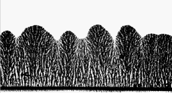
Figure 1: The Finger morphology 403 s after the start of the experiment. The solid black line at the bottom of the image is the cathode. The width of the image corresponds to 22.1 mm. The deposit was grown in a cell of 250 $\mu$m thickness, the applied potential was 15 V. The electrolyte contained 50 mM $\mathrm{CuSO_{4}}$ and 4 mM $\mathrm{Na_{2}SO_{4}}$.

The organization of the paper is the following: In Section II we introduce the experimental setups. Section III is devoted to the dispersion relations, with III.1 covering some technical aspects and III.2 presenting the measured dispersion relations and analyzing the results for a textured electrode. In Section IV we discuss the PIV measurements: IV.1 is devoted to the anode while IV.2 summarizes our results for the cathode. Finally, Section V contains our conclusions.

II Experimental Setups

The electrodeposition is performed in a cell with two glass plates of 8 x 8 $\mathrm{cm^{2}}$ area as side-walls. Two parallel copper wires (99.9 %, Goodfellow) separated by a distance of 4 cm serve as electrodes and spacers. Their diameter $d$ ranges between 125 $\mu$m and 300 $\mu$m. Figure 2 a) shows a sketch of this setup. We use a coordinate system where the x axis is parallel to the electrode, the y axis points from the cathode to the anode and the z axis is perpendicular to the glass plates.

The space between the electrodes is filled with an aqueous solution of 50 mM $\mathrm{CuSO_{4}}$ and 4 mM $\mathrm{Na_{2}SO_{4}}$ for the measurements of the dispersion relations and 50 mM $\mathrm{CuSO_{4}}$ and 7 mM $\mathrm{Na_{2}SO_{4}}$ for the PIV experiments. All solutions are prepared from Merck p.a. chemicals in non deaerated ultrapure $\mathrm{H_{2}O}$.

All measurements are performed with constant (within 0.4 %) potential between the electrodes ranging between 12 V and 19 V. The average current density is below 35 $\mathrm{mA/cm^{2}}$.

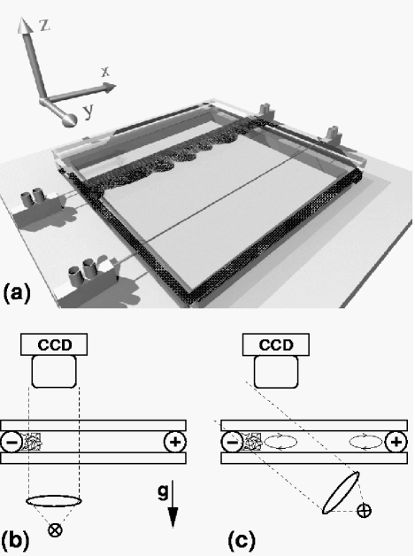
Figure 2: (a) Electrodeposition cell with finger deposit and our choice of the coordinate system. (b) Side view of the illumination with shining-through light used for the measurements of the dispersion relation. Image 1 was taken that way. (c) Side view of the dark field microscopy used for the PIV. Image 3 gives an example of this illumination technique. The ovals inside the cell indicate the convection rolls.

	CCD-camera	Pixel	optical system	resolution	$\Delta t_{aq}$
DR	Kodak	x: 3070	Nikkor 105/2.8	7.9 $\mu$m	5 s
	Megaplus 6.3i	y: 2048	SLR lens
PIV	Sony	x: 512	Olympus SZH	17 $\mu$m	2 s
	XC 77RR CE	y: 512	microscope

Table 1: Image acquisition systems used in the experimental setups.

The two targets of our investigation require two different ways of illumination (sketched in Fig. 2 (b) and (c)) and image acquisition (summarized in table 1). Since the measurements of the dispersion relation demand a high spatial resolution we used a Kodak Megaplus 6.3i CCD-camera with 3070 x 2048 pixel mounted on a Nikkor SLR macro lens with 105 mm focal length and a spacer ring. To take full advantage of the spatial resolution of 7.9 $\mu$m per pixel it was necessary to employ a Köhler illumination Göke (1988) using filtered light with a wave length of 405 nm from a tungsten lamp. Images are taken in intervals $\Delta t_{aq}$ of 5 s and are directly transferred with a frame-grabber card to the hard disk of a PC.

To visualize the velocity field inside the cell, we added latex tracer particles to the electrolyte. We used particles with 0.3 $\mu$m diameter, which stay suspended due to Brownian motion. Since we cannot resolve these particles with our optical system, we used dark-field microscopy: only light scattered from objects inside the cell falls into the lens. Image 3 gives an example, the white area at the bottom represents the growing deposit, the points above correspond to tracer particles.

We did not observe electro-osmosis as reported in Huth et al. (1995), but the particles show some tendency to coagulate and settle to the bottom plate. This problem is handled in later stages of the image processing.

Images were acquired using an Olympus SZH stereo microscope and a Sony XC 77RR CE CCD-camera with 512 x 512 pixels which resulted in a spatial resolution of 17 $\mu$m per pixel. $\Delta t_{aq}$ was 2 s and images were also directly transferred to a PC.

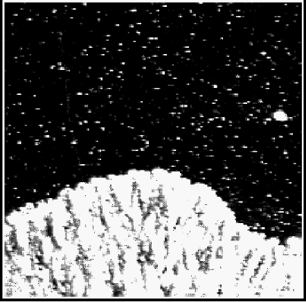
Figure 3: Part of an image taken in dark-field microscopy. Only light scattered from the deposit or the tracer particles is visible. The width corresponds to 3.4 mm. (Cell thickness: 300 $\mu$m, applied potential: 12 V, solution: 50 mM $\mathrm{CuSO_{4}}$ and 7 mM $\mathrm{Na_{2}SO_{4}}$.)

III Dispersion relation

To characterize the instability of a pattern forming systems there is a quite common method: starting with the uniform system, one adds a small sinusoidal perturbation of wavenumber $k$ and amplitude $A_{0}$ and investigates its temporal evolution. As long as the system is in the linear regime the perturbation will grow or shrink exponentially:

$$A(k,t)=A_{0}\;e^{\sigma(k)\;t}$$ (1)

The dependency of the growth rate $\sigma$ on the wavenumber $k$ is called dispersion relation.

In the context of electrodeposition dispersion relations have been measured for the initial phase of compact Kahanda et al. (1992) and ramified de Bruyn (1996) growth and calculated to explain the stability of the dense radial morphology Grier and Mueth (1993).

III.1 Image processing

In order to measure the dispersion relation the first step is to track down the temporal evolution of the front: in the image taken at time $t$ we identify for each column $x$ the height $h(x,t)$ of the deposit. This is done in two steps: First we search for the pair of pixels with the highest gray value gradient in each column. Second we perform a sub-pixel interpolation by calculating the point of inflexion between these two pixels. By evaluating a stationary edge, we could demonstrate that the error of this algorithm is smaller than 0.1 pixel. However the random fine structure of the deposit acts like the addition of shot noise to $h(x,t)$. We try to mitigate this effect by applying a median filter with 7 pixel width Jähne (1997). Figure 4 shows $h(x,t)$ for 4 various times of an experiment.

Figure 4: Result $h(x,t)$ of the front tracking. The curve at the bottom corresponds to the initial position of the cathode. Above the front at 156 s, 259 s, 362 s and 466 s after the beginning of the experiment. The experiment is the same as the one presented in Fig. 1. The part of length $w$ between the dashed lines was chosen by the cut-out algorithm for further processing.

Our next aim is to do a Fourier decomposition of $h(x,t)$ to examine the dynamics of the amplitudes $A(t,m)$ of the individual modes $m$. Because our initial conditions are random noise, which can be understood as a superposition of various modes with different wavelengths $\lambda$, we encounter a leakage problem: We observe our system in a window of width $w_{0}$. The ratio $w_{0}/\lambda$ of the dominant modes is almost always fractional. This has a very unpleasant consequence for the Fourier transformation, which computes the amplitudes for integer mode numbers: power of the dominant modes is transfered to other less excited modes and spoils the measurement of the growth rates there.

A common answer to this issue is the usage of a windowing function Harris (1978), which does not eliminate leakage, but restricts it to neighboring mode numbers. The price to be paid is, that this leakage will now occur even if $w_{0}$ is a common multiple of all wavelengths contained in the initial signal.

In this paper we use a different approach, which is illustrated in Fig. 4: we cut out a part of $h(x,t)$ of width $w$ and offset $o$ and use only this part for the subsequent analysis. $o$ and $w$, which are constant for the whole run of the experiment, are chosen such that the left and the right end of the cut-out have the same height:

$$h(o,t)-h(o+w,t)=0$$ (2)

and the same slope:

$$\frac{\partial h(o,t)}{\partial x}-\frac{\partial h(o+w,t)}{\partial x}=0$$ (3)

Fulfilling Eq. 2 and Eq. 3 for all times is for all practical purposes identical to the statement that $w$ is a common multiple of all wavelengths contained in $h(x,t)$, that is the condition under which no leakage occurs.

In practice, Eq. 2 and Eq. 3 can be satisfied only approximately. The algorithm followed to select $o$ and $w$ minimizes the sum over the height differences according to Eq. 2 while it assures, that the sum over the slope differences according to Eq. 3 does not exceed a threshold. The average height difference obtained in that way is $\leq$ 3 pixels while the slope difference threshold was 1 pixel/pixel, both values correspond to the noise level of $h(x,t)$. The final step is a standard Fourier decomposition of the cut-out parts of $h(x,t)$.

III.2 Results

For each Fourier amplitude we tried to fit the temporal evolution with the exponential growth law given by Eq. 1. Fig. 5 gives an example for two modes, corresponding to the experiment displayed in Fig. 4. The time interval for the exponential fits is indicated by the solid symbols. The start time is set by the time the hydrogel layer needs to build up; before that point no instability or destabilization of the growing interface is clearly evidenced. In the experiment shown in Fig. 4 this point corresponds to an elapsed time of about 150 s. However some modes need longer until they are grown to an amplitude which can be distinguished from the measurement background noise. At the other end the fit is limited by the onset of deviations from the exponential growth law due to nonlinear effects becoming important.

Figure 5: Exponential growth of the Fourier modes. The wave numbers are 6.9 $\mathrm{cm^{-1}}$ (circles) and 13.8 $\mathrm{cm^{-1}}$ (squares). Only the data points represented by filled symbols were included in the fits with Eq. 1. The experiment is the same as in Fig. 4.

To test the dependence of the dispersion relation on the applied potential, we performed measurements with 15 V and 19 V using electrodes of 250 $\mu$m diameter. The results are displayed in Fig 6, each is averaged over three experiments. Both dispersion relations show a limited band of positive amplitude growth rates with $k$ between zero and $k_{\mathrm{crit}}$ and a wave number $k_{\mathrm{max}}$ where the growth rate is maximal.

The increase of $U$ from 15 V to 19 V is accompanied by an increase of the average growth velocity $v$ from 13.3 $\mu$m/s to 15.9 $\mu$m/s. The distinct shift of $k_{\mathrm{max}}$ to higher wave numbers is in conformity with measurements of the number of incipient fingers as a function of $v$ reported in Lòpez-Salvans et al. (1996). The decrease of $k_{\mathrm{crit}}$ could originate from a change of the physicochemical properties of the copper hydrogel.

Figure 6: Dependence of the dispersion relation on the applied potential. Filled circles correspond to experiments performed applying 15 V, open circles applying 19 V. Cell thickness was 250 $\mu$m in both cases. All data sets are averaged over three experiments, error bars give the standard deviation of the mean value.

Negative “growth rates” can only be measured if the initial amplitude of the corresponding mode is strong enough. To enforce this we prepared a textured electrode which stimulates the initial growth at a wavenumber of 62.8 $\mathrm{cm^{-1}}$. It consists of a synthetic substrate of 120 $\mu$m height with a 35 $\mu$m copper plating. The copper layer was etched to derive a comb-like structure with copper stripes of width 0.75 mm and spacings of 0.25 mm. Islands of growing deposit evolve at the tips of the copper stripes and amalgamate after some time. Fig. 7 gives an example. The temporal evolution of two Fourier modes of this experiment is shown in Fig. 8.

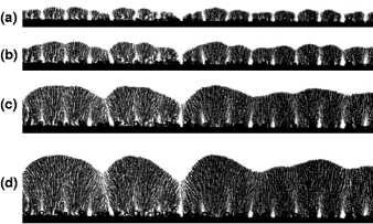
Figure 7: Growing deposit at the textured electrode. Images were taken (a) 51 s, (b) 82 s, (c) 142 s, (d) 202s after the beginning of the experiment. The width of the images corresponds to 15.8 mm. (Applied potential: 15 V, cell thickness 155 $\mu$m, solution: 50 mM $\mathrm{CuSO_{4}}$ and 7 mM $\mathrm{Na_{2}SO_{4}}$.)

Figure 8: Temporal evolution of the Fourier amplitudes measured with the textured electrode. The data belong to the experiment displayed in Fig. 7. The wavenumbers are 3.5 $\mathrm{cm^{-1}}$ (squares) and 62.6 $\mathrm{cm^{-1}}$ (circles). Data points represented by filled symbols were included in the fits with Eq. 1.

The dispersion relation of the textured electrode is displayed in Fig 9 together with results for cell thickness of 125 $\mu$m and 250 $\mu$m. Within the scope of our experimental errors no influence of $d$ is observable. In principle a decrease of $d$ is accompanied by a decrease of the surface tension forces, which should result in a higher $k_{\mathrm{crit}}$. However as discussed in chapter IV convection will also be significantly reduced. This will result in a steeper transition between the hydrogel and the electrolyte, which increases the surface tension $\gamma$ Smith et al. (1981). Presumably these two effects cancel each other.

Figure 9: Dependence of the dispersion relation on the cell thickness. Open circles were measured in cells with $d$ = 250 $\mu$m, open squares in cells with $d$ = 125 $\mu$m. The closed circles give the results of the textured electrode ($d$ = 155 $\mu$m). The solid line is a fit of Eq. 4 to the growth rates of the textured electrode. Applied potential was 15 V in all cases. All data sets are averaged over three experiments, error bars give the standard deviation of the mean value.

While we are not claiming that the Saffman-Taylor dispersion relation:

$$\sigma=\frac{(\eta_{\mathrm{g}el}-\eta_{\mathrm{H}_{2}0})v}{\eta_{\mathrm{g}el}+\eta_{\mathrm{H}_{2}0}}k-\frac{d^{2}\gamma}{12(\eta_{\mathrm{g}el}+\eta_{\mathrm{H}_{2}0})}k^{3}$$ (4)

gives a full explanation of this fingering phenomenon, we do believe that it captures the essentials of the physical mechanism, especially the damping effects due to an effective surface tension. Therefore we performed a fit of Eq. 4 to the dispersion relation of the textured electrode, which is shown in Fig. 9. As results we find a viscosity of the hydrogel $\eta_{\mathrm{g}el}$ of 2.4 $10^{-3}$ kg/ms which is about twice the viscosity of water $\eta_{\mathrm{H}_{2}0}$. The effective surface tension $\gamma$ turns out to be 3.5 $10^{-7}$ N/m. This is about five magnitudes lower than the surface tension at the water-air interface, which is presumably due to the fact, that the gel and the water are miscible fluids.

IV Velocity measurements

Electrodeposition is often accompanied by buoyancy-driven convection rolls Rosso et al. (1994); Barkey et al. (1994); Huth et al. (1995); Linehan and de Bruyn (1995); Chazalviel et al. (1996); Argoul et al. (1996); Lòpez-Salvans et al. (1997b); Dengra et al. (2000). The driving force for the convection are the concentration changes at the electrodes: at the anode the ion concentration and therefore the density of the electrolyte increases. While it descends, lighter bulk solution flows in and a convection roll as sketched in Fig 2 (c) starts to grow.

To visualize the growing deposit in the $x$-$y$ plane, we observe the cells from above. As apparent from Fig. 2 (c) the plane defined by the convection roll is the $y$-$z$ plane. This results in the uncomfortable situation, that the observed tracer particles move simultaneously towards and away from the electrode, which obviates the use of standard correlation techniques Raffel et al. (1998) for the PIV.

We therefore developed a software package capable to keep track of the motion of individual particles. This is done in two steps: First we identify the particles in each image and insert their center of mass into a database. Then we construct contiguous histories for individual particles using five consecutive time-steps. In this way we are able to measure the $v_{\rm x}$ and $v_{\rm y}$ components of the flow. The software is published under the GNU Public License and can be downloaded from a URL dow .

IV.1 Anode Results

All velocity measurements were performed in cells with thickness $d$ = 300 $\mu$m applying a potential of 12 V. At the anode a convection roll is clearly visible: while having no relevant velocity component in the $x$-direction, the tracer particles in a distinct zone move towards or away from the electrode. Fig. 10 gives the $v_{\rm y}$ components of all particles detected in one image as a function of their distance $y$ to the anode.

Figure 10: Particle velocities at the anode after 888 s. Particles with positive $v_{\mathrm{y}}$ are moving away from, with negative $v_{\rm y}$ towards the anode. Only particles lying outside the solid lines were considered for the calculation of an average velocity $v_{\mathrm{avg}}$. The dashed line is a fit of Eq. 10 to $v_{\mathrm{avg}}(y,t)$. The applied potential is 12 V, the cell thickness 300 $\mu$m.

Due to the big depth of focus of our optical system, we observe particles in all heights $z$ of the cell simultaneously. As the particle velocity is a function of $z$, we find for a given $y$ all velocities between $\pm v_{\mathrm{max}}(y,t)$.

IV.1.1 Theory

It is known that some time after the start of an experiment vertical diffusion starts to smear out the concentration differences between the flows to and away from the electrode. Chazalviel and coworkers Chazalviel et al. (1996) proposed a two-dimensional description for this diffusion-hindered spreading (DHS) regime. The velocity component perpendicular to the electrode $v_{\rm y}$ should obey exc :

$$v_{\rm y}(y,z,t)= k_{1}\;\left[\left(1-\frac{y}{k_{2}\;\sqrt{t}}\right)^{\nicefrac{{1}}{{2}}}-\frac{1}{12}\left(1-\frac{y}{k_{2}\;\sqrt{t}}\right)^{\nicefrac{{3}}{{2}}}\right]$$ (5)

$$\left(z^{3}-z\frac{d^{2}}{4}\right)$$

with

$$k_{1}=13.1\left(\frac{i\;\mu_{\mathrm{a}}\;\frac{\partial\rho}{\partial c}\;g}{z_{\mathrm{c}}\;F\;(\mu_{\mathrm{a}}+\mu_{\mathrm{c}})\;\eta}\right)^{\nicefrac{{1}}{{3}}}\;\frac{D^{\nicefrac{{1}}{{3}}}}{d^{\nicefrac{{8}}{{3}}}}$$ (6)

and

$$k_{2}=0.222\left(\frac{i\;\mu_{\mathrm{a}}\;\frac{\partial\rho}{\partial c}\;g}{z_{\mathrm{c}}\;F\;(\mu_{\mathrm{a}}+\mu_{\mathrm{c}})\;\eta}\right)^{\nicefrac{{1}}{{3}}}\;\frac{d^{\nicefrac{{4}}{{3}}}}{D^{\nicefrac{{1}}{{6}}}}$$ (7)

$i$ denotes the current density (25 $\pm$ 3 mA/$\mathrm{cm^{2}}$), $\frac{\partial\rho}{\partial c}$ is the dependency of the density on the ion concentration, which we measured to be 0.156 $\pm$ 0.008 kg/Mol for $\rm CuSO_{4}$ using a density measurement instrument DMA 5000 from Anton Paar. $\mu_{\rm a}$ and $\mu_{\rm c}$ represent the mobility of the anions (8.3 $10^{-8}$ $\mathrm{m}^{2}$/sV) and cations (5.6 $10^{-8}$ $\mathrm{m}^{2}$/sV), respectively. $F$ is the Faraday constant (9.6 $10^{4}$ As/Mol), $g$ the acceleration due to gravity and $z_{\mathrm{c}}$ the charge number of the cation (2). $\eta$ represents the dynamic viscosity ($10^{-3}$ kg/ms) of the solution and $D$ the ambipolar diffusion constant (8.6 $10^{-10}$ $\rm m^{2}$/s for $\rm CuSO_{4}$ Lide (1994)). Because $D$ and $\eta$ are weakly concentration dependent, we assign them errors of 10 % in the subsequent calculations, further on we assume a 5 % error in the determination of $d$. Eq. 5 assumes, that the glass plates are at $z=\pm d/2$ and $y$ = 0 at the anode.

Within this theory the extension $L$ of the convection roll is given by the point, where $v_{\rm y}(y,t)$ drops to zero:

$$L=k_{2}\>\sqrt{t}$$ (8)

The maximal velocity $v_{\rm max}$ occurs at the heights $z=\pm d/2\sqrt{3}$, in the immediate neighborhood of the electrode $(y=0)$, and is time independent:

$$v_{\rm max}=0.63\left(\frac{i\;\mu_{\mathrm{a}}\;\frac{\partial\rho}{\partial c}\;g\;d\;D}{z_{\mathrm{c}}\;F\;(\mu_{\mathrm{a}}+\mu_{\mathrm{c}})\;\eta}\right)^{\nicefrac{{1}}{{3}}}$$ (9)

However the authors state that due to problems with the boundary conditions at the electrode their solution might be not applicable in the region $0<y<d$.

IV.1.2 Test of the theory

In principle the theory should describe directly our experimental results, however due to the uncertainties in the parameters we decided to perform a fit. Because we measure a two-dimensional projection of velocities, we concentrate on an average velocity $v_{\rm avg}(y,t)$, which we calculate from all particles with absolute velocities of at least half the velocity of the fastest particle in this distance. In Fig 10 this corresponds to all particles not lying between the two solid lines. This restriction is necessary to remove the contribution of particles which have already settled to the bottom glass plate.

From Eq. 5 we derive our fit function:

$$v_{\mathrm{avg}}(y,t)=v_{0}\left[\left(1-\frac{y}{L}\right)^{\nicefrac{{1}}{{2}}}-\frac{1}{12}\left(1-\frac{y}{L}\right)^{\nicefrac{{3}}{{2}}}\right]$$ (10)

The fit of Eq. 10 to $v_{\rm avg}(y,t)$ is successful for the whole run of the experiment, especially the roll length $L$ is determined very precisely. Fig. 11 illustrates the temporal evolution of $L$ obtained from the fit. After 70 s $v_{0,\mathrm{exp}}$ becomes constant at a value of 24.7 $\pm$ 0.5 $\mu$m/s. Integrating Eq. 5 yields $v_{0,\mathrm{theo}}$ = 30.8 $\pm$ 2.1 $\mu$m/s.

Figure 11: Length $L$ of the convection roll at the anode. $L$ was determined by fitting $v_{\mathrm{avg}}(y,t)$ with Eq. 10. The two fits to the left and right of the dashed line have slopes of 0.7 $\pm$ 0.01 and 0.543 $\pm$ 0.001 where the errors are the asymptotic standard errors derived from the covariance matrix of the fit Press et al. (1992). The experiment is the same as presented in Fig. 10.

The next step is testing Eq. 8, which predicts the growth law of $L$. A fit of our experimental $L$ for times greater 75 s using equation $L(t)=k_{2,fit}t^{b}$ yields a slope of 0.543 $\pm$ 0.001, which is slightly above the square root law suggested by Eq. 8. Higher exponents have also been reported by other groups: Argoul et al. Argoul et al. (1996) found 0.56 $\pm$ 0.01 and Dengra et al. Dengra et al. (2000) measured 0.54 $\pm$ 0.02. The coefficient $k_{2,fit}$ was found to be 141 $\pm$ 1 $\mu$m/$\rm s^{\nicefrac{{1}}{{2}}}$. If we insert our experimental parameters in Eq. 7 we obtain $k_{2}$ = 134 $\pm$ 12 $\mu$m/$\mathrm{s}^{\nicefrac{{1}}{{2}}}$ in agreement with the fit.

Fig. 13 (b) shows the experimental results for the maximal fluid velocity, which is located in the vicinity of the anode. After a sharp rise at the beginning of the experiment follows a slightly inclined plateau. A linear fit yields a velocity of 25.5 $\pm$ 0.1 $\mu$m/s for $t$ = 0, which increases at a rate of 1 % per minute. Inserting the experimental parameters into Eq. 9 results in a constant velocity of 37.1 $\pm$ 2.5 $\mu$m/s. This discrepancy can be attributed to the unphysical boundary conditions used in the model.

Summarizing it can be stated, that the theory presented in Chazalviel et al. (1996) provides a qualitatively and semi-quantitatively good description of the anodic convection roll in the DHS regime.

IV.1.3 Initial phase of development

Apart from the DHS regime, Fig. 11 also shows a growth law $L\sim t^{0.7}$ for times between 12 s and 75 s. The exponent of 0.7 $\pm$ 0.01 indicates a faster growth originating from a different mechanism. In the very beginning of an experiment convective fluid transport is faster than the diffusive equalization between the copper ion enriched electrolyte and the bulk electrolyte. Therefore the concentrated electrolyte at the electrode sinks down and spreads along the bottom plate without significant mixing. In this so called immiscible fluid (IF) regime the length $L$ of the convection zone is expected to grow with $t^{\nicefrac{{4}}{{5}}}$. This has been shown for gravity currents Chen (1980); Huppert (1982) and was successfully adapted for electrodeposition Huth et al. (1995); Chazalviel et al. (1996). As explained in detail below, the range of applicability of this theory requires in our case $L<$ 470 $\mu$m, which is out of our measured range. Thus we observe a transitional period between the IF and the DHS regime and not the IF regime itself.

To distinguish between the IF and the DHS regime a scaling analysis based on the vertical diffusion time was used in Huth et al. (1995). We would like to advocate a different approach, using the similarity of the driving mechanism with the well-investigated case of a side heated box filled with fluid Cormack et al. (1974); Imberger (1974); Patterson and Imberger (1980). While in this case the density changes are due to thermal expansion, there exist also two flow regimes: In the so called convective regime small layers of fluid spread along the confining plates with a stagnant core in the middle of the cell. The conductive regime is characterized by a cell filling convection roll and iso-density lines which are almost vertical. These flows can be described by the Rayleigh number $Ra=\alpha\Delta T\rho gd^{3}/\kappa\eta$ and the aspect ratio $A=d/W$. $\alpha$ is the thermal expansion and $\kappa$ the thermal diffusivity of the fluid. $W$ denotes the distance, $\Delta T$ the temperature difference between hot and cold side wall. Boehrer Boehrer (1997) pointed out, that $Ra\,A^{2}$, which equals the ratio between the timescales for vertical diffusion and horizontal convection, is the dimensionless control parameter of this transition. For high values of $Ra\,A^{2}$ one observes the convective regime, for small values the conductive one.

If we transfer this analysis to our situation, we have to substitute the thermal density difference $\alpha\Delta T\rho$ with the density difference due to concentration changes $\frac{\partial\rho}{\partial c}c_{0}$ and the thermal diffusivity $\kappa$ with the ambipolar diffusivity $D$. This yields a concentration-dependent Rayleigh number $Ra_{\rm c}$ expressed by:

$$Ra_{\rm c}=\frac{\frac{\partial\rho}{\partial c}\;c_{0}\;g\;d^{3}}{D\;\eta}$$ (11)

The aspect ratio is calculated using the length of the convection roll: $A=d/L$. Analyzing the results presented in Fig 10 of Ref. Huth et al. (1995) this interpretation provides a necessary condition given by:

$$Ra_{\rm c}\,A^{2}>1000$$ (12)

to observe the IF regime. In our experiment $Ra_{\rm c}\,A^{2}$ will only be larger than 1000 for $L<$ 470 $\mu$m , which is out of our measured range.

IV.2 Cathode Results

At the cathode the situation is more complex due to the growing deposit. In Fig. 12 the solid line describes the position of the most advanced point of the deposit in a width of 2.3 mm in $x$-direction, while the dotted line corresponds to the minimum in the same interval. The border of the convection roll was measured using a threshold: the open circles mark the foremost position, where the $v_{y}$ component of a particle exceeded 4.3 $\mu$m/s.

While the convection roll develops immediately, no growth of the deposit is observable in the first 40 s, because the copper deposits in a planar compact way, which is not observable with our optical resolution. During this so called Sand’s time, the ion concentration at the cathode drops to zero, which subsequently destabilizes the planar growth mode Argoul et al. (1996).

In the next phase (40 s $<t<280$ s) a depth of the deposit (distance between the most advanced and most retarded parts of the growing deposit) becomes measurable and finally reaches a constant size. The advancing deposit significantly compresses the size $L$ of the convection roll as given by the distance between the dots and the solid line. Within this time interval the hydrogel layer is established, which can be seen by visual inspection.

The third phase ($t>280$ s) is characterized by the appearance of the finger development. The front minimum (dashed line) and maximum (solid line) in Fig. 12 coincide to the finger tip and the neighboring valley. The length $L$ of the convection roll in front of the finger tip tends to converge to a constant size, which has also been observed in the absence of a gel Huth et al. (1995); Chazalviel et al. (1996); Dengra et al. (2000). The dispersion relations studied in chapter III.2 were obtained in this phase.

Figure 12: Temporal evolution at the cathode. The solid line describes the position of a finger tip, the dashed line of a neighboring valley. The circles mark the leading edge of the convection roll. The experimental conditions are: $U$ = 12 V and $d$ = 300 $\mu$m.

Fig. 13 is devoted to a comparison between the flow behavior at the two electrodes. The developments of $L$ displayed in Fig. 13 (a) differ significantly from each other. However the comparison of the maximal fluid velocities in Fig. 13 (b) show similarities with respect to the absolute value and the approximate temporal constance. The fit at the cathode yields a velocity of 23.6 $\pm$ 0.3 $\mu$m/s for $t$ = 0 s, which decreases 0.9 % per minute.

From Fig. 13 (a) we infer, that the theoretical description presented in Chazalviel et al. (1996) cannot be applied to the cathode. Indeed three prerequisites of the theory are not fulfilled: Most importantly, it does not consider the moving boundary originating from the growth process. Moreover this model can lead to unphysical negative concentrations at the cathode due to its inherent simplifications. Finally the theory is two-dimensional in the $y$-$z$ plane and therefore not able to describe the influence of the ramified deposit, which evolves in the $x$-$y$ plane.

Figure 13: Comparison of the flow behavior at the two electrodes under identical experimental conditions. Filled circles correspond to the anode (Fig. 11), open circles to the cathode (Fig. 12). Part (a) shows the temporal evolution of the overall length $L$ of the convection roll. Part (b) gives the temporal evolution of the maximal velocity in y direction inside the rolls. The solid lines are fits to all data points with t $>$ 100 s.

Remarkably enough our measurements show that the presence of hydrogel does not prevent convection. For a better understanding of the contribution of the flow field to the finger morphogenesis, we visualize it in Fig. 14 for two different times of the same experiment. The solid line denotes the interface of the deposit, and the arrows indicate the velocity of individual particles. It is apparent that convection is restricted to a small zone in front of the growing deposit. The hydrogel occurs also in the immediate vicinity of the front, however its extension could not be investigated in any detail here.

Figure 14: Flow field at (a) 493 s and (b) 760 s after the beginning of the experiment. All particles detected in one image with a velocity $>$ 4.8 $\mu$m/s were included. Arrowheads have been omitted for clarity, the length of the lines corresponds to the way the particles travel in 6 s. ($U$ = 12 V, $d$ = 300 $\mu$m.)

To examine the orientation of the flow field with respect to the interface we first computed the distribution of the angle $\alpha$ between the velocity vectors $\mathbf{v}_{i}$ of the particles and the $y$ axis. These data correspond to the thin lines shown in Fig. 15. The distribution clearly broadens with time and exhibits two distinct maxima for the fully developed fingers analyzed in Fig. 15 (c).

Then we identified for each particle an associated point of the finger envelope by prolonging $\mathbf{v}_{i}$. The angle between the normal vector at this meeting point and the $y$ axis is labeled $\beta$. The angle difference $\alpha-\beta$ is a measure for the mismatch between the deposit and the convection roll and is displayed as the thick line in Fig. 15.

Fig. 15 (b) reveals that the convection field has a mismatch of about 15 degrees to the front during the initial phase of finger development. Thus we conclude that the development of the convection field lags behind the development of the front. After the fingers are fully developed, the convection field readjusts again perpendicularly to the interface as shown in Fig. 15 (c), which is a sign of the concentration gradient adapting to the geometry of the deposit.

Due to the lack of comparable measurements of other electrodeposition systems we can not judge if this effect is due to hydrogel or a generic feature of the cathodic convection roll.

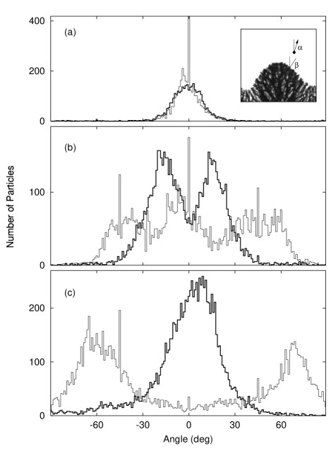
Figure 15: Angle histograms for the times (a) 3-97 s, (b) 493-651 s and (c) 730-918 s. The thin line gives the distribution of the angle $\alpha$ between the velocity vector $\mathbf{v}$ of a particle and the $y$ axis. Prolonging $\mathbf{v}$ we determine the meeting point with the finger surface. Its normal vector encloses the angle $\beta$ with the $y$ axis. The thick line shows the distribution of the angle difference $\alpha-\beta$. These data correspond to the experiment presented in Fig. 14.

V Summary and conclusions

We measured the dispersion relation in the linear regime of the finger morphology and their dependence on cell thickness and applied potential. By means of a textured electrode, we were able to measure negative growth rates. The striking feature of the smooth finger envelope is connected with the existence of a limited band of wavenumber between 0 an $k_{\mathrm{crit}}$ with positive growth rates. The damping of all perturbations with higher wavenumbers can be attributed to an effective surface tension associated with a hydrogel boundary in front of the deposit A fit of the dispersion relation yields some estimates for the effective surface tension and the viscosity of the copper hydrogel.

Furthermore we performed PIV measurement at both electrodes. At the anode we could confirm the $t^{\nicefrac{{1}}{{2}}}$ growth law for the length $L$ of the convection roll. We determined $L$ by fitting the suggested analytic expression for the velocity field and could therefore successfully test the model proposed by Chazalviel and coworkers.

At the cathode the maximal fluid velocity inside the convection roll is of the same order as at the anode, but the temporal evolution of $L$ differs strongly. An analysis of the orientation of the velocity vectors reveals the existence of some mismatch between the development of the convection roll and the deposit front while the system is in the linear regime. In the fully developed finger regime, the velocity vectors are again perpendicular to the envelope of the deposit.

Our results provide a reasonable explanation why in the absence of gravity-driven convection rolls the fingering instability cannot be observed: without convective mixing, the concentration gradient at the hydrogel interface can be assumed to be steeper, which will increases the effective surface tension. In consequence $k_{\mathrm{crit}}$ shifts to smaller wavenumbers and the overall growth rates decrease, which will suppress the evolution of fingers.

An alternative explanation assumes two zones within the hydrogel layer. One part of the hydrogel in immediate vicinity of the deposit will be mixed by the convection roll and the consequential shear thinning will decrease its viscosity. In front of it there is a zone of quiescent hydrogel of higher viscosity, at the interface between this two the instability takes place. In this scenario $k_{\mathrm{crit}}$ is determined by the length of the convection roll $L$.

A fully quantitative theoretical analysis remains to be done.

- (1) G. Binnig, talk at the Nobel Laureate Meeting in Lindau, Germany.
- Sagués et al. (2000) F. Sagués, M. Q. Lòpez-Salvans, and J. Claret, Physics Reports 337, 97 (2000).
- Trigueros et al. (1994) P. P. Trigueros, F. Sagués, and J. Claret, Phys. Rev. E 49, 4328 (1994).
- Lòpez-Salvans et al. (1996) M.-Q. Lòpez-Salvans, P. P. Trigueros, S. Vallmitjana, J. Claret, and F. Sagués, Phys. Rev. Lett. 76, 4062 (1996).
- Lòpez-Salvans et al. (1997a) M.-Q. Lòpez-Salvans, F. Sagués, J. Claret, and J. Bassas, J. Electroanal. Chem. 421, 205 (1997a).
- McCloud and Maher (1995) K. V. McCloud and J. V. Maher, Physics Reports 260, 139 (1995).
- (7) J. Fernandez, P.Kurowski, P.Petitjeans, and E. Meiburg, to be published in J. Fluid Mech.
- Göke (1988) G. Göke, Moderne Methoden der Lichtmikroskopie (Franckh’sche Verlagshandlung, Stuttgart, 1988).
- Huth et al. (1995) J. M. Huth, H. L. Swinney, W. D. McCormick, A. Kuhn, and F. Argoul, Phys. Rev. E 51, 3444 (1995).
- Kahanda et al. (1992) G. L. M. K. S. Kahanda, X. Zou, R. Farrell, and P. Wong, Phys. Rev. Lett. 68, 3741 (1992).
- de Bruyn (1996) J. R. de Bruyn, Phys. Rev. E 53, 5561 (1996).
- Grier and Mueth (1993) D. G. Grier and D. Mueth, Phys. Rev. E 48, 3841 (1993).
- Jähne (1997) B. Jähne, Digital Image Processing (Springer, Berlin, 1997).
- Harris (1978) F. J. Harris, Proceedings of the IEEE 66, 51 (1978).
- Smith et al. (1981) P. G. Smith, T. G. M. V. D. Ven, and S. G. Mason, Journal of Colloid and Interface Science 80, 302 (1981).
- Rosso et al. (1994) M. Rosso, J. N. Chazalviel, V. Fleury, and E. Chassaing, Elektrochimica Acta 39, 507 (1994).
- Barkey et al. (1994) D. P. Barkey, D. Watt, and S. Raber, J. Electrochem. Soc. 141, 1206 (1994).
- Linehan and de Bruyn (1995) K. A. Linehan and J. R. de Bruyn, Can. J. Phys. 73, 177 (1995).
- Chazalviel et al. (1996) J. N. Chazalviel, M. Rosso, E. Chassaing, and V. Fleury, J. Electroanal. Chem. 407, 61 (1996).
- Argoul et al. (1996) F. Argoul, E. Freysz, A. Kuhn, C. Léger, and L. Potin, Phys. Rev. E 53, 1777 (1996).
- Lòpez-Salvans et al. (1997b) M.-Q. Lòpez-Salvans, F. Sagués, J. Claret, and J. Bassas, Phys. Rev. E 56, 6869 (1997b).
- Dengra et al. (2000) S. Dengra, G. Marshall, and F. Molina, J. Phys. Soc. Jpn. 69, 963 (2000).
- Raffel et al. (1998) M. Raffel, C. E. Willert, and J. Kompenhans, Particle Image Velocimetry (Springer, Berlin, 1998).
- (24) http://itp.nat.uni-magdeburg.de/matthias/piv.html.
- (25) The anion migration velocity used in Ref Chazalviel et al. (1996) is difficult to access experimentally. Therefore we did substitute it by the currrent density using Eq. 5 and Eq. 8 in Ref Chazalviel et al. (1996): .
- Lide (1994) D. R. Lide, ed., CRC Handbook of Chemistry and Physics (CRC Press, Boca Raton, 1994), 75th ed.
- Press et al. (1992) W. H. Press, S. A. Teukolsky, W. T. Vetterling, and B. P. Flannery, Numerical Recipes in C, Second Edition (Cambridge University Press, 1992), chap. 15.6.
- Chen (1980) J.-C. Chen, Ph.D. thesis, California Institute of Technology, Pasadena, California (1980).
- Huppert (1982) H. E. Huppert, J. Fluid Mech. 121, 43 (1982).
- Cormack et al. (1974) D. E. Cormack, L. G. Leal, and J. Imberger, J. Fluid Mech. 65, 209 (1974).
- Imberger (1974) J. Imberger, J. Fluid Mech. 65, 247 (1974).
- Patterson and Imberger (1980) J. Patterson and J. Imberger, J. Fluid Mech. 100, 65 (1980).
- Boehrer (1997) B. Boehrer, Int. J. Heat Mass Transfer 40, 4105 (1997).