Spectral properties of quantized barrier billiards

Abstract

The properties of energy levels in a family of classically pseudointegrable systems, the barrier billiards, are investigated. An extensive numerical study of nearest-neighbor spacing distributions, next-to-nearest spacing distributions, number variances, spectral form factors, and the level dynamics is carried out. For a special member of the billiard family, the form factor is calculated analytically for small arguments in the diagonal approximation. All results together are consistent with the so-called semi-Poisson statistics.

I Introduction

Two decades after the first investigation of the quantum mechanics of nonintegrable polygonal billiards RichensBerry81, a renewed interest in this peculiar class of dynamical systems has shown up recently. One reason is the fabrication of polygonal-shaped optical microcavities VKLISLA98; BGRFRKDK98; BILNSSVWW00; PCC01. Another reason is the finding BGS99; BGS01b that certain planar rational polygons (all angles between sides are of the form $p\pi/q$, where $p$, $q$ are relatively prime integers) have spectral properties very similar to those of mesoscopic disordered systems at the critical point of the metal-insulator transition SSSLS93 and to those of systems with interacting electrons WWP99.

The classical dynamics in rational polygons having at least one critical corner with $p>1$ is characterized as pseudointegrable RichensBerry81. The phase space is foliated by two-dimensional invariant surfaces Hobson75; ZemlyakovKatok75, like in integrable systems Arnold78, but the genus of the surfaces is larger than one RichensBerry81. The flow on these surfaces is typically ergodic and not mixing Gutkin96.

Pseudointegrable systems cannot be quantized according to the semiclassical Einstein-Brillouin-Keller rule RichensBerry81. As a consequence, the statistical properties of energy levels of classically pseudointegrable systems are different from those of integrable systems which are generically well described by Poissonian random processes BerryTabor77a. For example, the nearest-neighbor spacing distribution of pseudointegrable systems generically displays a clear level repulsion RichensBerry81 as in the case of the Gaussian orthogonal ensemble (GOE) of random-matrix theory Mehta67 which describes fully chaotic systems with time-reversal symmetry BGS84. Significant deviations from GOE are observed first theoretically SS93 and later experimentally in microwave cavities SSSSSZ94.

Recently, the semi-Poisson (SP) statistics have been proposed as reference point for the spectral statistics of pseudointegrable systems BGS99; BGS01b. Following HFS99; BGS01b, we define SP statistics by removing every other level from an ordered Poisson sequence $\{x_{n}\}$. Unfortunately, the term “semi-Poisson” was originally coined for a sequence $\{y_{n}\}$ where $y_{n}=(x_{n}+x_{n+1})/2$ BGS99. We call this here interpolated-Poisson (IP) statistics. IP and SP statistics have identical nearest-neighbor spacing distributions but other spectral quantities in general differ.

The SP conjecture has been verified numerically for right triangular BGS99; BGS01b and rhombus billiards GremaudJain98 where only small differences to SP have been found. However, numerical works on right triangles in a regime of high level numbers seem to indicate that the statistical properties are nonstationary Gorin01; PG01 with increasing, but still small, deviations from SP as the energy is increased PG01. For certain right triangles, it has been shown analytically that the spectral form factor for small arguments is located around the corresponding SP result BGS01.

However, the triangles studied in BGS01 are not generic rational polygons, because they belong to the class of Veech polygons Veech89 which may have special spectral properties. In this paper, we study the symmetric barrier billiards Zwanzig83; HM90; Wiersig00; Wiersig01; ZE01; EMS01; Wiersig01b where the even-symmetry states, the “pure barrier-billiard states”, are expected to show the generic behavior. We provide analytical and extensive numerical calculations showing that the spectral properties are fully consistent with SP statistics. Moreover, our results throw some light on the nonstationarity observed in Gorin01; PG01.

The paper is organized as follows. After defining the billiard family in Sec. II, we compute analytically the form factor for small arguments in Sec. III. Numerical results are presented in Sec. IV. Section V contains a conclusion.

II Barrier billiards

The family of barrier billiards consists of rectangles with sizes $l_{x}$, $l_{y}$ and a barrier placed on the symmetry line $x=l_{x}/2$ as shown in Fig. 1(a). The length of the barrier $l\in(0,l_{y})$ is the only nontrivial parameter. The free motion of a point particle with mass $m$ and momentum $(p_{x},p_{y})$ bounded by elastic reflections at the boundary of the billiard has a second constant of motion $K=p_{x}^{2}$ in addition to Hamilton’s function $H$. Hence, the dynamics in phase space is restricted to invariant surfaces $(H,K)=\text{constant}$. The topology of these surfaces is not that of a torus (with genus 1) but that of a two-handled sphere (genus 2) due to the critical corner at the upper end of the barrier; see RichensBerry81 for the relation between critical corners and the genus of invariant surfaces in pseudointegrable billiards.

The billiards are Veech (roughly speaking, this property implies a special kind of hidden symmetry) if and only if $l/l_{y}$ is a rational number EMS01. Still, a typical symmetric barrier billiard is not a generic pseudointegrable system since it is composed of two copies of an integrable sub-billiard, the rectangle shown in Fig. 1(b). This property is identical to almost-integrability Gutkin86 in the case of $l/l_{y}$ being rational.

Figure 1: (a) Trajectory (dotted) in the full barrier billiard, a rectangle with a barrier between the points $(x,y)=(l_{x}/2,0)$ and $(l_{x}/2,l)$. Symmetry-reduced system with (b) Dirichlet boundary conditions and (c) mixed boundary conditions: Dirichlet (Neumann) on solid (dashed) lines.

The energy eigenstates are solutions of the Helmholtz equation with Dirichlet boundary conditions, i.e. vanishing amplitude, on the boundary of the polygon. The states are odd or even with respect to the symmetry line. The former ones are trivial eigenstates of the integrable sub-billiard in Fig. 1(b). We therefore deal mainly with the even ones, the “pure barrier-billiard states”, which fulfill mixed boundary conditions on the boundary of the symmetry-reduced polygon; see Fig. 1(c). We expect that the pure barrier-billiard states show the generic features of energy states in rational polygons.

III The spectral form factor

We here compute analytically a spectral quantity, the 2-point correlation form factor, for the energy levels $\{E_{n}\}$ of a special member of the barrier-billiard family. Our calculation is inspired by that for the triangular billiards in BGS01. It turns out that the present calculation is much simpler. As in BGS01, we will apply the modern semiclassical theory based on trace formulas which express the density of states of a quantum system in terms of periodic orbits of the underlying classical system Gutz90. For billiards, the semiclassical limit $\hbar\to 0$ corresponds to the high-energy limit $E\to\infty$. Throughout the paper we use natural units such that $\hbar=2m=1$.

The density of states can be written as sum of a smooth part and an oscillatory part

$$d(E)=\sum_{n}\delta(E-E_{n})=\bar{d}(E)+d_{\text{\footnotesize osc}}(E).$$ (1)

The fluctuations in the oscillatory part can be studied with the help of the 2-point correlation function

$$R(\epsilon)=\left<{d_{\text{\footnotesize osc}}(E+\frac{\epsilon}{2})}{d_{\text{\footnotesize osc}}(E-\frac{\epsilon}{2})}\right>\ .$$ (2)

Brackets $\langle\ldots\rangle$ denote an energy averaging around $E$ on an energy window much larger than the mean level spacing $1/\bar{d}(E)$, and much smaller than $E$. The Fourier transform of $R(\epsilon)$ is the spectral form factor

$$K(\tau)=\int_{-\infty}^{\infty}\frac{d\epsilon}{\bar{d}}R(\epsilon)e^{2\pi i\bar{d}\epsilon\tau}\ .$$ (3)

We will concentrate on the limit $\tau\to 0$; $K(0)=1$ for Poisson Berry85b, $1/2$ for SP BGS01 and $0$ for GOE Berry85b; Mehta67.

For two-dimensional rational polygons, the smooth part of the density of states is semiclassically described by Weyl’s law $\bar{d}=A/(4\pi)$ where $A$ is the area of the polygon; the oscillating part splits into two parts VWR94; PS95

$$d_{\text{\footnotesize osc}}(E)=d_{\text{\footnotesize p.o.}}(E)+d_{\text{\footnotesize d.o.}}(E)\ .$$ (4)

The periodic orbit contribution

$$d_{\text{\footnotesize p.o.}}(E)=\sum_{\text{\footnotesize p.o.}}\frac{A_{p}}{4\pi}\frac{1}{\sqrt{2\pi kl_{p}}}e^{ikl_{p}-i\nu_{p}\pi/2-i\pi/4}+c.c.$$ (5)

is a summation over classical (primitive and non-primitive) periodic orbits. These orbits are marginally stable and appear always in one-parameter families reflecting the foliation of phase space by two-dimensional invariant surfaces. $p$ labels these families; $A_{p}$ denotes the surface in configuration space covered by a given family (without repetitions of primitive periodic orbits); $l_{p}$ is the (non-primitive) length of periodic orbits; the Maslov index $\nu_{p}$ is here twice the number of reflections at Dirichlet boundaries (Neumann boundaries do not contribute); $k=\sqrt{E}$ is the wave number.

The diffractive orbit contribution $d_{\text{\footnotesize d.o.}}(E)$ is a summation over orbits starting and ending at critical corners of the polygon. This summation is more involved than the periodic orbit contribution BPS00. In the limit $\tau\to 0$, however, the form factor $K(\tau)$ does not depend on diffractive orbits BGS01. With this insight a formula for $K(0)$ has been derived in BGS01 by inserting the periodic orbit contribution (5) into Eq. (3) and employing the diagonal approximation (which is expected to be valid for small $\tau$) yielding

$$K(0)=\lim_{\tau\to 0}\frac{1}{8\pi^{2}\bar{d}}\sum_{\text{\footnotesize p.o.}}\frac{|A_{p}|^{2}}{l_{p}}g_{p}^{2}\delta(l_{p}-4\pi k\bar{d}\tau)\ ,$$ (6)

where $g_{p}$ is the multiplicity of a given periodic-orbit family, i.e. the number of families with exactly the same lengths, and the summation is performed over families with different lengths.

For later considerations it is helpful to repeat the evaluation of Eq. (6) for the simplest case, the rectangular billiard, as done in BGS01. A family of periodic orbits in a rectangle with sizes $a$, $b$ ($a$ and $b$ are irrationally related) and area $A=ab$ can be specified by two non-negative integers $m_{p}$ and $n_{p}$, denoting the number of traversals across the billiard in the $x$- and $y$-direction, respectively. The length of each orbit is

$$l_{p}=\sqrt{(2m_{p}a)^{2}+(2n_{p}b)^{2}}\ .$$ (7)

The number of periodic orbits $N(l)$ up to length $l$ is the number of lattice points in the positive $(m_{p},n_{p})$-quadrant inside the ellipse (7) asymptotically giving by

$$N(l)=\frac{\pi l^{2}}{16A}\ .$$ (8)

Due to the fact that all families cover the same area $A_{p}=2A$ and have typically the same multiplicity $g_{p}=2$ (time-reversal symmetry) the sum (6) can be replaced by the following simple integral

$$K(0)=\lim_{\tau\to 0}\frac{2A^{2}}{\pi^{2}\bar{d}}\int_{0}^{\infty}\frac{1}{l}\delta(l-4\pi k\bar{d}\tau)\frac{dN(l)}{dl}dl$$ (9)

which gives $K(0)=1$ as expected for generic integrable systems Berry85b.

We now extend the previous calculation to the barrier billiard. To keep the calculation elementary, we restrict ourself to the special Veech case $l=l_{y}/2$. The odd states are eigenstates in the rectangle with width $a=l_{x}/2$, height $b=l_{y}$, and with Dirichlet boundary conditions, see Fig. 1(b), so we get $K(0)=1$ as demonstrated above. The even states, the “pure barrier-billiard states”, fulfill mixed boundary conditions as shown in Fig. 1(c). In the semiclassical trace formula (5), the inhomogeneous boundary conditions only influence the Maslov indices of the periodic orbits: a reflection at a Dirichlet boundary increases the index by two in contrast to a reflection at a Neumann boundary which does not change the index. The resulting phase difference of $\pi$ between trajectories has an analog in billiards with a magnetic flux line BGS01 where trajectories encircling a flux of 1/2 (in natural units) once pickup a phase $\pi$.

First, let us consider periodic orbits with fixed $m_{p},n_{p}\geq 0$ and $m_{p}$ odd. We write $m_{p}=m_{N}+m_{D}$ where $m_{N},m_{D}\geq 0$ count the number of reflections at $x=l_{x}/2$ with Neumann or Dirichlet boundary condition, respectively. Two cases have to be distinguished: $m_{N}$ even and $m_{D}$ odd; $m_{N}$ odd and $m_{D}$ even. The corresponding two types of orbits are related by a symmetry transformation (ignoring the boundary conditions), the reflection at the line $y=l_{y}/2$. Hence, both types have the same $l_{p}$, $g_{p}$ and $A_{p}$. However, the Maslov indices are different due to the inhomogeneous boundary conditions: $\nu_{p}\,{\rm mod}\,4=0$ and $\nu_{p}\,{\rm mod}\,4=2$, respectively. This implies that the contribution of both families to the trace formula (5) are identical differing just by a sign. Therefore both contributions cancel each other.

Second, let us turn to periodic orbits with $m_{p}$ even. We begin with unfolding the orbits into a larger rectangle with width $a^{\prime}=2a$. Assume, for simplicity, that $m_{p}^{\prime}=m_{p}/2$ is odd. The case $m_{p}^{\prime}$ even can be treated by further unfolding of the orbits. Again, for $m_{p}^{\prime}=m_{N}^{\prime}+m_{D}^{\prime}$ odd there exists two kinds of periodic orbits related by symmetry: one with $m_{N}^{\prime}$ even and $m_{D}^{\prime}$ odd and one with $m_{N}^{\prime}$ odd and $m_{D}^{\prime}$ even. These two kinds of trajectories either become congruent or remain separated when folded back into the original rectangle with width $a$. In the first case, we have to add the two different values of $m_{N}^{\prime}$ and the two values of $m_{D}^{\prime}$ leading to $m_{N}$ and $m_{D}$ odd throughout the family. In the other case, we get $m_{N}=2m_{N}^{\prime}$ and $m_{D}=2m_{D}^{\prime}$ even since each orbit is symmetric with respect to the folding axis. Clearly, for fixed $n_{p}$ only one of these two cases is possible. Hence, no cancellation occurs for even $m_{p}$ in the trace formula (5), in contrast to the complete cancellation in the case of $m_{p}$ odd. The simple consequence of which is that the number of periodic-orbit families which contributes to the trace formula (5) is reduced by a factor two. The same is true for the sum (6). From Eq. (9) follows then directly our main analytical result

$$K(0)=\frac{1}{2}\ .$$ (10)

Our calculated $K(0)$ is not only close to the SP prediction as in the case of Veech triangles BGS01, it agrees exactly with the SP prediction.

The calculation for general barrier length is considerably more complicated. Yet, it should be possible to compute $K(0)$ also for rational $l/l_{y}\neq 1/2$ using methods developed in BGS01; EMS01.

IV Numerical results

We here present numerical results on several statistical quantities for general symmetric barrier billiards. As representatives we choose the Veech billiard with $l=l_{y}/2$ and one which is not Veech with $l=l_{y}\omega$, where $\omega=(\sqrt{5}-1)/2$ is (the reciprocal of) the golden mean. Irrationally related parameters $l_{x}=\pi\sqrt{8\pi}/3$ and $l_{y}=3\sqrt{8\pi}/\pi$ are taken. Billiards with $l\approx 0$ and $l\approx l_{y}$ are not investigated since the semiclassical behavior of these limiting cases is expected to set in at extremely high energies. We consider two different energy regimes: (i) the medium-energy regime starting with the $40\,000$th level and ending with the $60\,000$th level, and (ii) the high-energy regime starting with the $400\,000$th level and ending with the $420\,000$th level. Our high-energy regime is below that of Ref. PG01 and above that of Ref. Gorin01.

We compute the eigenvalues with the mode-matching technique which is very efficient for barrier billiards as described in detail in Wiersig01. An accuracy of about $10^{-4}$ of the mean level spacing is achieved.

To distinguish between local fluctuations in the level sequence $E_{1}\leq E_{2}\leq E_{3}\leq\ldots$ and a systematic global energy dependence of the average density we “unfold” the spectra in the usual way by setting $\tilde{E}_{n}=\bar{N}(E_{n})$; see, e.g., Haake91. $\bar{N}(E)$ is the smooth part of the integrated density of states $N(E)=\int d(E^{\prime})dE^{\prime}$ (number of levels up to energy $E$). In contrast to our semiclassical analysis in the previous section, we have to take into consideration that our energy regime is finite, therefore we approximate $\bar{N}(E)$ by the generalized Weyl’s law including perimeter and corner corrections BH76. We obtain for the rectangle with Dirichlet boundary conditions in Fig. 1(b)

$$\bar{N}(E)=E-\frac{l_{x}+2l_{y}}{4\pi}\sqrt{E}+\frac{4}{16}$$ (11)

and for the rectangle with mixed boundary conditions in Fig. 1(c)

$$\bar{N}(E)=E-\frac{l_{x}+2l}{4\pi}\sqrt{E}+\frac{1}{16}\ .$$ (12)

By construction, the unfolded spectra $\{\tilde{E}_{n}\}$ have unit mean level spacing. Henceforth, the tilde $\tilde{}$ will be suppressed.

IV.1 Nearest-neighbor spacing distributions

An important statistical quantity measuring short-range level correlations is the nearest-neighbor spacing distribution. It is defined as the probability density of the spacing $s$ between adjacent levels

$$P(s)=\lim_{n\to\infty}\frac{1}{n}\sum_{i=1}^{n}\delta(s-E_{i+1}+E_{i})\ .$$ (13)

We will compute its integral, the cumulative spacing distribution

$$I(s)=\int_{0}^{s}P(s^{\prime})ds^{\prime}\ .$$ (14)

For Poisson statistics $P_{\text{\footnotesize P}}(s)=\exp{(-s)}$ and $I_{\text{\footnotesize P}}(s)=1-\exp{(-s)}$, the GOE is well described by the Wigner surmise $P_{\text{\footnotesize W}}(s)=(\pi/2)s\exp{(-\pi s^{2}/4)}$ and $I_{\text{\footnotesize W}}(s)=1-\exp{(-\pi s^{2}/4)}$, and for the SP statistics HFS99; BGS01b

$$P_{\text{\footnotesize SP}}(s)=4se^{-2s},\,\,I_{\text{\footnotesize SP}}(s)=1-(2s+1)e^{-2s}\ .$$ (15)

$P_{\text{\footnotesize SP}}(s)$ shows a linear increase at small $s$ (level repulsion) like the Wigner surmise and an exponential fall-off at large $s$ like Poisson statistics.

In Fig. 2 one sees that the cumulative spacing distribution is in good agreement with the SP statistics in both energy regimes (the medium-energy behavior of the non-Veech billiard is not shown since it is similar to the Veech case). However, small fluctuations around SP can be observed in the magnification. The fluctuations decrease with increasing energy, and they are larger than the statistical fluctuations $<0.5/\sqrt{W}\approx 0.0035$ due to the finite width $W=20\,000$ of the energy windows. For the Veech billiard, we find a slight tendency towards the Wigner surmise for medium energies and a slight tendency towards the Poisson distribution for high energies. The fluctuations in the non-Veech case are of the same magnitude but without clear tendency towards Wigner surmise or Poisson distribution.

Figure 2: Difference between the cumulative spacing distribution of the pure barrier-billiard levels. Below: magnification.

The fluctuations for the Veech barrier billiard are very similar (but by a factor 2.5 smaller in the high-energy regime) than those found in right triangles PG01. In PG01, increasing fluctuations have been reported for very high energies above the $4\,000\,000$th level. These fluctuations have been interpreted as deviations from SP leading to the conclusion that SP is asymptotically not the relevant statistics for pseudointegrable systems. In the following paragraphs, however, we will show that this interpretation is doubtful.

Let us construct an artifical SP distributed sequence of numbers. Take the levels of the simple rectangle in Fig. 1(b) given by

$$E^{0}_{mn}=(2\pi m/l_{x})^{2}+(\pi n/l_{y})^{2}$$ (16)

with $m,n=1,2,3,\ldots$. It has been demonstrated numerically that the nearest-neighbor spacing distribution and some other statistical properties of such a sequence are asymptotically extremely well described by the Poisson statistics RobnikVeble98; see also Marklof98. After ordering the levels according to increasing energy and removing every other level, the nearest-neighbor spacing distribution of the sequence thus obtained obeys SP statistics HFS99. Figure 3 shows the corresponding cumulative spacing distribution computed numerically from $20\,000$ levels in three different regimes. The medium- and high-energy regime are defined as before, whereas the very-high-energy regime starts at the $4\,000\,000$th level as in Ref. PG01. We observe small fluctuations around SP which decrease with increasing energy. In the medium- and high-energy regime, the fluctuations are of the same order of magnitude as for the pure barrier-billiard levels; cf. Fig. 2. We note that the same fluctuations are also present when $I(s)-I_{\text{P}}(s)$ is plotted for the Poisson sequence given by Eq. (16).

The statistical fluctuations depend on the number of levels under consideration. This carries over to the total fluctuations as illustrated for the very-high-energy regime in Fig. 3 with $10\,000$ and $20\,000$ levels, respectively. Hence, one should not compare the statistics of sequences with different number of levels as it has been done in PG01.

Following the same reasoning as described above we have also constructed a SP sequence of $20\,000$ numbers using a conventional pseudo-random number generator. This reproduces the expected statistical fluctuations of order $0.0035$. To summarize, from the fluctuations found numerically here and in PG01; Gorin01 it is not justified to exclude SP as correct statistics for generic pseudointegrable systems.

Figure 3: Difference between the cumulative spacing distribution of the artifical SP sequence.

We mention that the distribution of spacings between neighboring eigenvalues of the S-matrix in an open version of the barrier billiard ESTV96 also resembles the SP result; although the agreement is not as good as here.

IV.2 Next-to-nearest spacing distributions

In the previous subsection we have seen that the nearest-neighbor distributions are close to the SP prediction in Eq. (15). However, Eq. (15) is also valid for IP statistics. In order to distinguish between IP and SP statistics one has to consider other correlation functions. First, we choose the next-to-nearest spacing distribution (second-neighbor-spacing distribution) and its integral. For the SP statistics BGS01b

$$P_{\text{\footnotesize SP}}(2,s) = \frac{8}{3}s^{3}e^{-2s}\,,$$

$$I_{\text{\footnotesize SP}}(2,s) = 1-\frac{1}{3}(4s^{3}+6s^{2}+6s+3)e^{-2s}\ .$$ (17)

For IP we find analytically

$$P_{\text{\footnotesize IP}}(2,s) = 4e^{-s}[1-(1+s)e^{-s}]\,,$$

$$I_{\text{\footnotesize IP}}(2,s) = 1+e^{-s}[e^{-s}(3+2s)-4]\ .$$ (18)

Figure 4 shows that the cumulative next-to-nearest spacing distribution is in agreement with the SP statistics but not with IP statistics. Note that the fluctuations are two times larger as in the case of the nearest-neighbor spacing distribution in Fig. 2.

Figure 4: Difference between the cumulative next-to-nearest spacing distribution of the pure barrier-billiard levels.

We have also investigated $n$th-neighbor spacing distributions $P(n,s)$ with $n=3,4,5$. Again, the distributions differ significantly from IP statistics and are well described by SP statistics, even though the fluctuations increase slightly. A detailed discussion is left out since we will study long-range level correlations in a more comprehensive way in the next subsection.

IV.3 Number variance

The number variance

$$\Sigma(L)=\left<(n(L,E)-L)^{2}\right>$$ (19)

is the local variance of the number $n(L,E)=N(E+L/2)-N(E-L/2)$ of energy levels in the interval $[E-L/2,E+L/2]$. SP statistics gives BGS99; HFS99; BGS01b

$$\Sigma_{\text{\footnotesize SP}}(L)=\frac{L}{2}+\frac{1}{8}(1-e^{-4L})\ .$$ (20)

For IP statistics we get analytically a different result

$$\Sigma_{\text{\footnotesize IP}}(L)=L-\frac{1}{2}+(L+\frac{1}{2})e^{-2L}\ .$$ (21)

Figure 5 reveals a substantial difference to SP for correlation lengths $L>4$ in the medium-energy regime. In the high-energy regime the difference is smaller. Note that the $L$ regime in Fig. 5 is well below the crossover region where the number variance begins to saturate at a value determined by the shortest periodic orbit Berry85b. In the region of large $L$, the number variance is related to the form factor (see, e.g., BGS01) by means of

$$K(0)=\lim_{L\to\infty}\frac{\Sigma(L)}{L}\ .$$ (22)

Using this relation we get for the Veech case $K(0)\approx 0.27$ at medium energies and $\approx 0.34$ at high energies ($\approx 0.36$ for the non-Veech case). However, we do not interpret this result as deviation from SP since we know from Section III that in the Veech case $K(0)$ does converge to the SP result $1/2$. Hence, we conclude that the convergence to a stationary limit is extremely slow. The slow convergence of the spectral statistics is shared by related systems such as right triangular billiards BGS01; Gorin01; PG01, rectangular billiards with magnetic flux lines BGS01; RF01, and parabolic maps with spin HK01. To overcome the problem of slow convergence, we have tried to use an extrapolation procedure described in BGS01. However, in our case it does not give satisfactory results and therefore a detailed discussion is omitted.

Figure 5: Number variance $\Sigma(L)$ of the pure barrier-billiard levels.

Figure 6 shows the number variance for the artifical SP sequence constructed from the levels of the integrable rectangle. The convergence in direction towards SP is similar, even though a bit faster, as for the pure barrier-billiard levels plotted in Fig. 5. In the regime of very high energies, the number variance is hard to distinguish from the SP curve.

Figure 6: Number variance $\Sigma(L)$ of the artifical SP sequence.

IV.4 The form factor

The form factor $K(\tau)$ can be approximated numerically by (see, e.g., Ref. Marklof98)

$$K(\tau;n)=\frac{1}{n}\left|\sum_{j=l}^{l+n}e^{2\pi iE_{j}\tau}\right|^{2}.$$ (23)

We here consider only the high-energy regime, i.e. $l=400\,000$ and $n=20\,000$. We smooth $K(\tau;n)$ by averaging over small intervals of size $\Delta\tau=0.006$. Nevertheless, the numerical data is quite irregular as can be seen in Fig. 7 for the Veech billiard (for the non-Veech case the picture looks very similar). It is difficult to estimate $K(0)$ directly from such kind of data, but it is clear that $K(0)$ is well below the SP prediction $1/2$, which is consistent with our former numerical results on the number variance.

A more elegant way to compare the form factor to SP statistics is described in Ref. BGS01. Fit $K(\tau;n)$ to the function

$$K_{\text{fit}}(\tau)=\frac{a^{2}-2a+4\pi^{2}\tau^{2}}{a^{2}+4\pi^{2}\tau^{2}}\ .$$ (24)

Expression (24) is the SP form factor when $a=4$. Therefore, the quantity $K_{\text{fit}}(0)-1/2$ measures the difference to SP statistics. Note that $K_{\text{fit}}(0)$ in general differs from $K(0;n)$ since it depends also on $K(\tau;n)$ with $\tau>0$. Fitting Eq. (24) to our smoothed data over the range $0\leq\tau\leq 3$, we find remarkable agreement with SP statistics: $K_{\text{fit}}(0)=0.504$ for the Veech billiard (see Fig. 7) and $K_{\text{fit}}(0)=0.498$ for the non-Veech billiard.

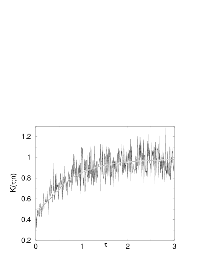
Figure 7: The form factor (23) of the pure barrier-billiard levels; $l=l_{y}/2$. The smooth curve is the fit (24) with $a=4.032$.

IV.5 Level dynamics

We here investigate the dependence of the energy levels on the system parameter $l/l_{y}$. This so-called “level dynamics” has been intensively studied for classically integrable and chaotic systems; see e.g. Haake91. To the author’s knowledge, only one pseudointegrable (for all parameter values) example, the “square torus billiard” RichensBerry81 and a generalized version of it SimmelEckert95, has been studied in this regard.

A typical situation for the pure barrier-billiard levels is displayed in Fig. 8. The global increase of the levels (not unfolded) is due to the fact that the smooth part of the integrated density of states in Eq. (12) decreases as $l$ is increased. Apart from this rather trivial fact we observe a number of interesting features: (i) the levels tend to avoid each other. Closer examination of the available numerical data indicates that there are no level crossings. That means for fixed parameter value there are no degeneracies in the spectrum, which is consistent with the SP and the GOE prediction for the nearest-neighbor spacing distribution $P(0)=0$ in agreement with our former numerical results. The total absence of level crossings is in contrast to the situation in the square torus billiard where crossings can appear for parameter values at which the billiard is almost integrable RichensBerry81. (ii) Large areas free of levels exist similar as in integrable systems and different to fully chaotic systems. This is consistent with Poisson and SP statistics which both predict a slower fall-off of $P(s)$ at large $s$ than GOE statistics does. (iii) There exists an unusual structure of plateaus interrupted by steep segments not only near avoided crossings but also fairly far away from avoided crossings. Observation of the energy eigenfunctions reveals that plateaus (steep segments) correspond to parameter values at which the corresponding eigenfunction has small (large) amplitude at the upper end of the barrier. Hence, varying the barrier length has no (strong) influence on the wave pattern and on the energy, resulting in a plateau (steep segment).

Figure 8: Pure barrier-billiard levels as functions of the barrier length $0.05l_{y}\leq l\leq 0.95l_{y}$.

Interestingly, the abrupt changes in the slopes fairly far away from avoided crossings can be simulated in a natural way by an artifical SP sequence constructed as described before by removing every other level of an integrable system. Two neighboring levels of an integrable system typically cross each other when a parameter is varied as sketched in Fig. 9. Removing the second level (measured from below for each value of the parameter) gives the solid, nondifferentiable line. This could produce the kind of abrupt changes seen in Fig. 8. Of course, the slope of finite-energy levels cannot change discontinuously. Real discontinuouities can only be expected in the semiclassical limit.

Figure 9: Sketch of the local level dynamics of the artifical SP sequence.

V Conclusion

In this paper we have studied the energy levels of pseudointegrable barrier billiards. Focusing on the pure barrier-billiard states, we have found numerically that the nearest-neighbor spacing distributions and next-to-nearest spacing distributions agree with the semi-Poisson (SP) statistics which is obtained by dropping every other number from a random sequence. The number variance and the spectral form factor agree with SP, even though long-range correlations seem to converge rather slowly. Moreover, the level dynamics is consistent with SP statistics. Even though we have considered an high-energy window ($20\,000$ levels starting at the $400\,000$th level) we cannot exclude that at larger energies a different scenario takes place. However, our analytical result for the spectral form factor for a Veech barrier billiard, $K(\tau)\to 1/2$ as $\tau\to 0$, gives us some confidence that the spectral statistics of barrier billiards are indeed close to SP.

Due to the slow convergence of the spectral statistics in polygonal billiards, and other diffractive systems, semiclassical methods as shown here and in BGS01 have to be extended in the future to higher order in $\tau$ (as in BG01 for rectangular billiards with point-like singularities) and to other polygons in order to clarify the role of the SP statistics in pseudointegrable systems.