Delayed Self-Synchronization in Homoclinic Chaos

Abstract

The chaotic spike train of a homoclinic dynamical system is self-synchronized by re-inserting a small fraction of the delayed output. Due to the sensitive nature of the homoclinic chaos to external perturbations, stabilization of very long periodic orbits is possible. On these orbits, the dynamics appears chaotic over a finite time, but then it repeats with a recurrence time that is slightly longer than the delay time. The effect, called delayed self-synchronization (DSS), displays analogies with neurodynamic events which occur in the build-up of long term memories.

PACS numbers : 05.45.Xt, 05.45.Vx, 42.65.Sf.

The last decade has seen a great interest in controlling chaos using small perturbations [1]. It started with the seminal paper by Grebogi, Ott, and Yorke [2] in which they proposed a method of stabilizing unstable periodic orbits using tiny, yet carefully chosen perturbations to an accessible system parameter. Subsequently, other methods were proposed, as the delayed feedback due to Pyragas [3], who showed that re-inserting a time-delayed version of the output back into the system can at certain conditions stabilize some of its periodic orbits. However, that method does not provide a reliable procedure that guarantees the stability of a chosen orbit, in particular it is exceedingly difficult to stabilize long periodic orbits. An improved version of the delayed feedback was represented by the adaptive control [4], experimentally implemented via a Taylor expansion which consists in feeding a delayed fraction of the output as well as its variation rate [5].

In this paper we show that for a chaotic system displaying a continuous return to a saddle focus (Shilnikov chaos [6]) and a high sensitivity to external perturbations applied near that focus, a long-delayed feedback can indeed be used to stabilize very complex sequences of pulses. We demonstrate this in numerical simulations and experiments with a CO2 laser as well as on a return map model of a chaotic pulse generator. However the validity of this scenario is much broader, including possible neurodynamic implications. We call this effect ”delayed self-synchronization” (DSS), insofar as the time signal appears as a train of N erratically distributed spikes (N being the ratio between the delay time and the average inter-spike interval) which repeat themselves with the same interspike intervals. The DSS phenomenon should by no means be confused with the synchronization of two distinct systems [7].

Standard control methods are of limited effectiveness for long times insofar as their complexity increases with the length of the periodic orbit, as shown e.g. by the Hunt’s occasional proportional feedback applied to long period orbits [8]. On the contrary, in DSS each return to the saddle focus permits an independent control of the corresponding inter-spike interval, and such an operation can be updated as long as one wishes, without any increase in complexity. In our laboratory implementation (Fig.1), a single-mode CO₂ laser with intensity feedback is tuned to the parameter range yielding homoclinic chaos [9]. The intensity output of the laser consists of a sequence of almost identical spikes, repeating at erratic times because of the homoclinic scrambling, with an average period of 500 $\mu s.$ (Fig. 2a). Through a delay unit described elsewhere [10], a small delayed perturbation (a few percent of the intensity output) is added to the feedback signal responsible for homoclinic chaos. As figures 2-b,c show, this small feedback creates a sequence of spikes, which is periodic with a period $T_{r}$ slightly larger than the delay time $T_{d}$ of the feedback loop (DSS). In fact, the DSS adjusts in such a way that the spikes of the delayed signal arrive through the delay line in the time interval of largest susceptibility, which occurs around $\tau\simeq 150\mu s.$ before the next large spike whence $T_{r}=T_{d}+\tau$ . The extra time or ”refractory time” $\tau$, which in fact corresponds to the duration of the quenched (zero intensity) time interval for each spike, is also measured by the width of the correlation function of the free running laser (Fig.3-a).

The autocorrelation function of the DSS signal has large revival peaks separated by the peiod $T_{r}$ (Fig. 3-b). Figure 4 shows that the minimal signal $\epsilon$ necessary for DSS is constant for long delays, down to a delay of $\tau\simeq 150\mu s$. For delays below the intrinsic refractory time $\tau$, the DSS threshold increases dramatically.

DSS can be further illustrated by the space-time representation (STR) introduced elsewhere [11]. In this representation, the time series is split into pieces of length $T_{r}$, which then are stacked together as different ”snapshots” of a 1D spatiotemporal system. Thus, every line of this representation is mapped onto the next line. The STR for the free-running system and for the DSS regime are shown in Fig. 5. When DSS is achieved, the STR of the dynamics changes drastically.

We also investigate DSS by a numerical experiment with the model of the homoclinic chaos in CO₂ laser, introduced earlier [12],

$$\begin{array}[]{l}\dot{x}_{1}=k_{0}x_{1}(x_{2}-1-k_{1}\sin^{2}(x_{6}))\\ \dot{x}_{2}=-\gamma_{1}x_{2}-2k_{0}x_{2}x_{1}+gx_{3}+x_{4}+p_{0}\\ \dot{x}_{3}=-\gamma_{1}x_{3}+x_{5}+gx_{2}+p_{0}\\ \dot{x}_{4}=-\gamma_{2}x_{4}+gx_{5}+zx_{2}+zp_{0}\\ \dot{x}_{5}=-\gamma_{2}x_{5}+zx_{3}+gx_{4}+zp_{0}\\ \dot{x}_{6}=-\beta(x_{6}+b_{0}-rX_{1})\end{array}$$ (1)

Here $x_{1}$ is the laser intensity, $x_{2}$ is the gain, $x_{3}$ , $x_{4}$, $x_{5}$ are variables of the gain medium, x6 is the feedback voltage, and $p_{0}$ is the pump rate. The delayed feedback is introduced in the equation for the feedback voltage $x_{6}$ via $X_{1}=x_{1}(t)+\varepsilon\cdot\left(x_{1}\left(t-T_{d}\right)-\bar{x}_{1}\right)$, where $\bar{x}_{1}$ is the mean value of $x_{1}(t)$. Parameters of the model at which the regime of homoclinic chaos is observed are $k_{0}=28.57$, $k_{1}=4.55$; $\gamma_{1}=10.06$, $\gamma_{2}=1.06$, $g=0.05$, $p_{0}=0.016$, $z=10$, $r=70$, $b_{0}=0.173$, $\beta=0.42$.

In numerical simulations, we are not limited in the length of the time delay and the time series. We ran very long simulations (up to $5\cdot 10^{6}$ non-dimensional time units) with long time delays up to 8000. The numerical time series (Fig. 6) are very similar to the experimental ones. The auto-correlation function also exhibits sharp peaks separated by a time interval $T_{r}$ that is slightly larger than $T_{d}$. The magnitude of the peaks very slowly decays with time, which indicates the slow evolution of the periodic orbit.

Notice that, once the dynamical system has become periodic with period $T_{r}=T_{d}+\tau$, that is, $x_{1}(t)=x_{1}(t-T_{r})$, than by Taylor expansion we can write $X_{1}=(1+\epsilon)\cdot x_{1}(t)+\epsilon\cdot(\frac{dx_{1}}{dt})\tau-\epsilon\cdot\bar{x}_{1}$. Thus for $\varepsilon=-1$, the delay feedback effect disappears as zero-th order term, as expected from Pyragas [3], but a first order correction proportional to the time derivative of $x_{1}$ represents the adaptive correction of Ref.[4] in the approximation of Ref.[5].

The DSS mechanism can be elucidated using the following simplified model. Without time-delayed feedback, after a pulse is produced, the phase trajectory spends some amount of time (which fluctuates because of the homoclinic chaos) near the homoclinic saddle before it leaves its neighborhood and produces the next pulse. A close inspection of the time series, both experimental and numerical (see Figs. 2-b,c and 6), indicates that the arrival of a pulse through the delay loop triggers the escape of the phase trajectory of the laser system from the neighborhood of the homoclinic saddle. Thus, the following simplified model can be proposed. Consider a system that generates a pulse at time $t_{i}$ , which is determined by a map

$$\begin{array}[]{l}t_{i}=t_{i-1}+f\left(t_{i-1}-t_{i-2}\right)\end{array}$$ (2)

If the function $f\left(\bullet\right)$ is chosen such that the map $x_{n+1}=f\left(x_{n}\right)$ produces chaos, then the sequence of pulses will be chaotic. Such system has actually been implemented in electronic circuitry [13]. Let us assume now that the pulses are inserted back into the system after a certain time delay $T_{0}$, so if a delayed pulse arrives at a time $t_{p}$ between $t_{i-1}+\delta$ and $t_{i}$, then it triggers a new pulse at $t_{p}$ instead of $t_{i}$, and the system is reset so that new $t_{i}=t_{p}$. We introduce the small offset $\delta$ in order to avoid spurious generation of pulses with very small time distance, which would effectively destroy pseudo-chaotic pulsation. In fact in the experiment this ”refractory time” was $T_{r}-T_{d}=150\mu s$. We iterated this system numerically using the logistic map $f\left(x\right)=ax\left(1-x\right)$ with $a=3.8$ and found that the system typically settles on a periodic orbit with the period $T_{0}$ as shown by its autocorrelation function (Fig.7). The particular orbit will obviously depend on initial conditions, in particular, orbits with periods much smaller than $T_{0}$, can also be stabilized, however they are not typical. Note, in this case the strength of the feedback is irrelevant as long as the magnitude of the pulses passed through the delay line is sufficient to trigger the next pulse. This agrees with the experimental observation that the threshold of synchronization is independent of $T_{0}$ for large enough $T_{0}$ (Fig. 4). We also checked the influence of noise on DSS. If noise was added to the sequence of the pulses at the levels below the threshold for pulse generation, it would not affect DSS. However, if a small white Gaussian noise is added to the inter-pulse interval, the revival peaks eventually decay to zero, albeit very slowly.

We have thus introduced a conceptual model for the phenomenon of delayed self-synchronization which leads to stabilization of very long-periodic orbits in a chaotic system. Such long orbits are known as a signature of the so-called pseudo-chaos observed in systems with discretized state space [14]. In those systems, the short-term behavior is indistinguishable from a real chaos, however the orbit returns to the initial point after some time and then repeats itself. Obviously, in the systems considered here, the state space is continuous, so the analogy between pseudo-chaos and DSS cannot be carried too far.

The ability to synchronize very long and complex periodic orbits is of particular interest in relation to the recent discovery of the neuronal mechanism of transformation of short-term memories into permanent (long-term) memories via so called synaptic reentry reinforcement (SRR) [15]. In those experiments, it has been demonstrated that neurons responsible for learning, repeatedly ”replay” certain spiking patterns in order to establish permanent connections (synapses) among neurons. We believe that stabilization of the complex periodic orbits in simple chaotic systems presented in this paper can serve as a paradigm for SRR in more complex neural systems. In our forthcoming work we will consider stabilization of long periodic orbits in the Hindmarsh-Rose neural model [16]. We believe that the homoclinic chaos observed in that system as well as in real biological neurons [17], is analogous to the laser chaos described here, and thus is should be susceptible to the phenomenon of delayed self-synchronization.

Authors are indebted to S. Boccaletti and N.F.Rulkov for useful discussions. F.T.A., R.M. and E.A. acknowledge partial support from the European Contract No. HPRN-CT-2000-158. A.D.G. is supported by European Contract No. PSS 1043. L.T. wants to thank Istituto Nazionale di Ottica Applicata (Florence) for warm hospitality. The work of L.T. was partially supported by the Engineering Research program of the Office of Basic Energy Sciences at the U.S. Department of Energy, grants DE-FG03-95ER14516 and DE-FG03-96ER14592 and by the UC MEXUS-CONACYT grant.

Figures

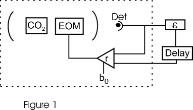
FIG. 1.: Experimental setup consisting of a CO₂ laser with a feedback loop (dashed line) imposing a regime of homoclinic chaos, and a delay unit. $EOM$, electro-optic modulator; $Det$, HgCdTe detector; $r$ and $b_{0}$, gain and bias of the amplifier in the feedback loop; $\epsilon$ and $Delay$, coupling factor and delay units.

FIG. 2.: A sequence of homoclinic spikes in the output intensity of a CO₂ laser in the free running regime (a) and DSS for two different delays (1 and 4 $ms$, (b) and (c) respectively). A thick arrow denote the zero intensity level. The two horizontal bars for 1 and 4 $ms$ show the role of the refractory time $\tau=150\mu s$. The shorter bar is the imposed delay ($T_{d}$), the larger one, with $\tau$ added, is the effective delay ($T_{r}$) that characterizes DSS.

FIG. 3.: Autocorrelation function of the laser intensity for the free running case (a) and for DSS with $T_{d}=4ms$ (b). The recurrence time $T_{r}$ for the revival of the correlation is the sum of $T_{d}$ plus the refractory time $\tau$.

FIG. 4.: Minimal DSS signal (in percent of the peak to peak output) versus the delay time.

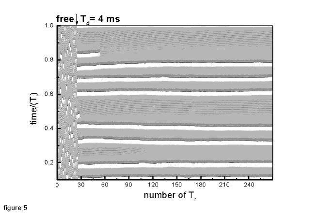
FIG. 5.: Space-time plots of the transition from free running to DSS regime with a delay time $T_{d}=4ms$ (indicated by the arrow). The space cell corresponds to a single recurrence time $T_{r}$, the time coordinate is a sequence of integer values corresponding to the successive delay units.

FIG. 6.: Numerical simulations of the laser equations (1) with time delay $T_{d}=2ms$: solid line, a section of the time series of the laser output; dotted line - the same time series shifted forward by the delay time $T_{d}$ and displaced vertically by $-1$. As clearly seen, the spikes of the delayed signal give rise to the rapid escape of the laser intensity from the floor at $0.5$ (denoted by a thich arrow), corresponding to the saddle-focus.

FIG. 7.: Autocorrelation function of the chaotic pulse generator (2) with delayed feedback. Sharp spikes are separated by the delay time $T_{0}=1000$.

REFERENCES

- [1] S. Boccaletti, C. Grebogi, Y.-C. Lai, H. Mancini and D. Maza, Physics Report 329, 103 (2000).
- [2] E.Ott, C.Grebogi, and J.Yorke, Phys. Rev. Lett. 64, 1196 (1990).
- [3] K.Pyragas, Phys. Lett, A 170, 421 (1992).
- [4] S. Boccaletti, and F.T. Arecchi, Europhys. Lett. 31, 127 (1995).
- [5] S. Boccaletti, D. Maza, H. Mancini, R. Genesio and F.T. Arecchi, Phys. Rev. Lett. 79, 5246 (1997); M. Ciofini, A. Labate, R. Meucci and F.T. Arecchi, Eur. Phys. J. D 7, 9 (1999).
- [6] L.P. Shilnikov, Sov. Math. Dokl. 6, 163 (1965).
- [7] V.S. Afraimovich, N.N Verichev and M.I. Rabinovich, Radiophys. Quant. Electron. 29, 795 (1986); L.M. Pecora and T.L. Carroll Phys Rev Lett. 76, 1916 (1996); M.G. Rosenblum, A.S. Pikovsky and J. Kurths, Phys.Rev. Lett. 78, 4193 (1997).
- [8] E.R. Hunt, Phys. rev. Lett. 67, 1953 (1991).
- [9] E. Allaria, F.T. Arecchi, A. Di Garbo and R. Meucci, Phys. Rev. Lett. 86, 791 (2001).
- [10] G. Giacomelli, R. Meucci, A. Politi and F.T. Arecchi, Phys. Rev. Lett. 73, 1099 (1994).
- [11] F.T. Arecchi, G. Giacomelli, A. Lapucci and R. Meucci, Phys. Rev. A 45, R4225 (1992).
- [12] A. N. Pisarchik, R. Meucci and F.T. Arecchi ”, Eur. Phys. J. D 13, 385 (2000).
- [13] N.F.Rulkov and A.R.Volkovskii, Phys. Lett. A 179, 332 (1993).
- [14] B. Chirikov and F. Vivaldi, Physica D 129, 223 (1999).
- [15] E. Shimizu, Y-P. Tang, C. Rampon and J.Z. Tsien, Science 290, 1170 (2000).
- [16] J. L. Hindmarsh and R. M. Rose, Proc. R. Soc. London, Ser. B 221, 87 (1984).
- [17] R.C. Elson, A.I. Selverston, R. Huerta, N.F. Rulkov, M.I. Rabinovich and H.D.I. Abarbanel, Phys. Rev. Lett. 81, 5692 (1998).