Olfactory search at high Reynolds number

Locating the source of odor in a turbulent environment — a common behavior for living organisms — is non-trivial because of the random nature of mixing. Here we analyze the statistical physics aspects of the problem and propose an efficient strategy for olfactory search which can work in turbulent plumes. The algorithm combines the maximum likelihood inference of the source position with an active search. Our approach provides the theoretical basis for the design of olfactory robots and the quantitative tools for the analysis of the observed olfactory search behavior of living creatures (e.g. odor modulated optomotor anemotaxis of moth).

Olfactory search strategies are interesting because of their relevance to animal behavior [1, 2, 3, 4, 5, 6] and because of their potential utility in practical applications (such as searching for chemical leaks, drugs and explosives [27]). Both, the attempt to characterize and understand the olfactory behavior of living organisms [1, 2, 3, 4, 5, 6] and the more recent effort to design and build “sniffing machines” — robots that navigate using odors as a guide [27, 26, 28, 29] — face the common problem of understanding how the information gained from sporadic detection of odor dispersed in a naturally turbulent flow can be efficiently utilized for locating the source. Here we shall discuss the statistical aspects of turbulent odor dispersal and propose a novel and well defined search algorithm, which we shall first define in the context of a simplified model of the turbulent plume and later restate in the form applicable to natural environment. The proposed search algorithm can be used in robotic applications and provides a plausible algorithmic interpretation for aspects of insect olfactory search behavior.

The most familiar strategy for locating the source of a substance is chemotaxis [7, 30] which consists of motion in the direction of the local concentration gradient. Chemotaxis works on small scales, where the substance spreads by diffusion and the field of concentration is smooth which is appropriate to the environment of bacteria, amoebae or single eukaryotic cells [30, 31]. On the other hand, larger animals tracing odors in turbulent flows, e.g. in atmosphere, have to deal with the complex fluctuating structure of the odor plume caused by the randomness in the flow which disperses it. This makes the search a much more complex task. The odor is not always present and when it is detected, the local concentration gradient typically does not point toward the source [2, 8, 9, 10, 11]. A more complex strategy is required and additional information such as the current wind direction (and velocity) is very valuable. One of the best characterized olfactory search behaviors is the ”odor-modulated optomotor anemotaxis”, which is employed by males of certain species of moths (see [1, 2]) in order to locate the source of a pheromone (i.e. potential mate), and which involves, in addition to the sense of smell, the ability to determine the wind direction. The moth’s olfactory pursuit flight exhibits a counterturning pattern: a succession of turns alternatively to left and right with respect to the wind direction. Counterturning is further classified as i) casting and ii) zigzagging [15, 16, 17, 18]. The two differ in the extent of upwind progression: ”zigzagging” is counterturning with a significant resultant movement upwind, while ”casting” is counterturning with no upwind progression but with wider cross-wind excursion. Casting and zigzagging behavior has been interpreted [15, 16] as a strategy consisting of upwind progression in the presence of odor (zigzagging) and cross-wind flight in its absence (casting). Most generally the two behavioral patterns may be understood in terms of ’exploitation’ and ’exploration’ [32]: the former utilizes the available information, the latter attempts to collect it. Below we shall identify the quantitative considerations which provide the rational basis for this type of behavior in the context of the olfactory search.

Let us first discuss the properties of odor plumes in turbulent flows [2, 13, 14]. If one measures the concentration of odor far enough downwind of the source, most of the time no odor will be detected [2] . When an odor patch arrives it is detected as a burst with a complicated small-scale structure, as local concentration fluctuates strongly while the patch is passing by. The maximal amplitude of the concentration within such a patch decreases away from the source, and the average time between two successive patches increases. The probability of encountering an odor patch at any given point is determined by the statistics of the flow. The mean velocity (and direction) of the wind, $V,$ is set by the large-scale atmospheric conditions and hence stays unchanged for periods of time long compared with the time-scale of odor fluctuations. The material points, and thus odor molecules, move with the local velocity which includes fluctuations about $V$ so that their net motion is a random walk (due to velocity fluctuations) superimposed on the drift downwind (due to mean velocity). The fluctuations of velocity have a correlation length, $L$, which can be estimated as the height above the ground (since the height above the ground restricts the size of the vortices) [10]. At scales larger than the correlation length $L$, the motion is effectively Brownian with the diffusion coefficient given by eddy-diffusivity, $D$ [21] which can be estimated as $Lv_{{\rm rms}}$, where $v_{{\rm rms}}$ is the root-mean-square of velocity fluctuations[10]. A patch of odor is blown as a whole along a Brownian trajectory and is stretched due to spatial inhomogeneity of the velocity. The stretching produces small-scale variations of the concentration of odor which decay due to molecular diffusion. Thus, odor patches have a finite life time due to mixing which occurs abruptly when the smallest scale of the patch reaches the Batchelor scale set by molecular diffusion [11]. Probability of a patch to survive for time $t$ in the flow is expected to behave as $e^{-tv_{{\rm rms}}/L}$. Because the fluctuating component of velocity is typically much smaller than the mean, $v_{rms}<<V,$ the probability of finding an odor patch at a downstream distance much larger than $L$ is still significant.

This Lagrangian view [11] of odor dispersal, in terms of relatively long-lived patches of odor exercising a biased random work, suggests the following model which will help us formulate the key issues relevant to olfactory search. Consider a square two-dimensional lattice. The sites have coordinates ${\bf r}=(x,y)$ and the source is at $(0,0)$. At each time step the source releases an ”odor patch” which is advected by the ”wind”. The wind velocity can take three values: $(-1,1)$, $(0,1)$, and $(1,1)$, so that the odor patch moves according to the following rule: each time step its $y$-coordinate increases by $1$ and $x$-coordinate gets incremented by $\pm 1$ or stays unchanged. The probabilities of the increments $-1$, $0$, and $1$ are $p_{{\rm L}}$, $p_{0}$, and $p_{{\rm R}}$. Without loss of generality we assume that $p_{{\rm L}}=p_{0}=p_{{\rm R}}=1/3$ , so that the average velocity points along $y$-axis. This model represents odor dispersion on the length scale larger than the correlation length, $L,$ which corresponds to the lattice constant in the model. The three dimensional structure of the real plume is not essential, because it does not dramatically change the statistical distribution of ’patches’. On the other hand, it is natural to conduct a two dimensional search (e.g. constant high above the ground) at least to within distance $L$ from the source. Hence our choice of a two-dimensional model.

Figure 1 shows a snapshot of a plume generated by the process described above. If we wait long enough, a stationary distribution of patches will be reached, which at $y\gg 1$ has the asymptotic form

$$p({\bf r})=\frac{1}{\sqrt{4\pi Dy}}\exp\left[-\frac{x^{2}}{4Dy}\right]\,,$$ (1)

where $D=(p_{{\rm R}}+p_{{\rm L}})/2$ is the ’eddy diffusivity’. The boundary of the time averaged plume has the form $|x|\approx\sqrt{Dy}$. The probability to find an odor patch at $x\gg\sqrt{Dy}$ is very small. On the other hand, at $x\lesssim\sqrt{Dy}$ the probability is of the order of $(4\pi Dy)^{-1/2}$.

Let us now define the search rules for the model plume. A local “observer” (our model moth or a robot) can detect a) the event of odor patch arrival, b) direction from which the patch has arrived. This corresponds in reality to the ability to detect instantaneous odor concentration and instantaneous wind velocity. Each time step, our robot is able to move at most one lattice step along $y$-axis and/or one lattice step along $x$ -axis. For simplicity we will assume that the robot does not move downwind, i.e. it does not increase its $y$-coordinate. The search starts after the robot contacts an odor patch for the first time.

Our goal is to find the best search algorithm. An algorithm must determine where the robot should move at the next moment based on, in principle, all prior observations. Each algorithm is characterized by the time it takes to find source — the search time. Due to random nature of the plume the search time is a random quantity. Hence we consider the probability distribution function of the search time, $\rho(t)$, given by the probability that the source is found during $t,t+1$ interval. For some algorithms the search time can be infinite in some realizations of the plume, which means the source is never found. Since each algorithm is characterized by a function, $\rho(t)$, and not by a number, the definition of the optimal algorithm is non-unique: one can choose different optimization criteria. Below we shall seek an efficient algorithm in the sense of the mean search time.

First consider a simple strategy, which will help to understand the more efficient one. Suppose that the robot waits at one site until it gets an odor patch. Then it moves to the site from which the patch came. This will always lead to the source, i.e. the probability to miss the source is zero for this strategy. It is possible to analytically calculate the probability density function (PDF) of the search time. Near the peak it has the Gaussian form

$$\rho(t)\approx\frac{1}{\sqrt{2\pi\Delta}}\exp\left\{-\frac{(t-t_{{\rm s}})^{2}}{2\Delta}\right\}\,,$$ (2)

$$t_{{\rm s}}\propto y_{0}^{3/2}\exp\left(\frac{x_{0}^{2}}{4Dy_{0}}\right)\,,\,\,\Delta\propto y_{0}^{2}\exp\left(\frac{x_{0}^{2}}{2Dy_{0}}\right)\,,$$

where ${\bf r}_{0}=(x_{0},y_{0})$ is the initial position of the robot, and $t_{{\rm s}}$ is the ’typical’ search time. In addition one can derive that for $t\gg t_{{\rm s}}$ PDF decays as $\rho(t)\propto t^{-3}$.

From this expression for the PDF one can see that the strategy has severe drawbacks. If the initial position is inside of the parabolic region, $x_{0}\lesssim\sqrt{Dy_{0}}$, the typical search time goes as $y_{0}^{3/2}$. However, from outside of the parabolic region $x_{0}\gtrsim\sqrt{Dy_{0}}$, the search time grows with $x_{0}$ faster than exponentially, $\exp\left(\frac{x_{0}^{2}}{4Dy_{0}}\right)$, which means that the strategy does not work well for points away from the plume axis. The PDF variance $\Delta$ also increases rapidly with $x_{0}$ and in addition the long time asymptotic form of the PDF is a power law, $\rho(t)\propto t^{-3}$, which mean that there exists a relatively high probability that the search takes much longer than the typical time, $t_{{\rm s}}$. This is explained by the robot’s tendency to get trapped outside of the parabolic region on the way towards the source.

The same drawbacks are inherent to the maximum likelihood algorithms [22, 23]. In these strategies one estimates the probability for the source to be located at any given point conditional on the history of observation and then move in the direction of the most likely source location. However, unless one waits for a long time so that many particles are observed, this conditional probability is a flat function of coordinates, i.e. many source locations around the maximum have approximately the same probability. As a consequence, all reliable algorithms of maximum likelihood type suffer from the drawbacks described above: i) the search time increases rapidly if the initial position is shifted outside of the parabolic region and ii) the probability that the search takes much longer than the mean time is substantial.

The inefficiency of the passive search algorithms is related to a small probability of encountering odor patches. To avoid this, one should not waste time waiting for odor patches which arrive rarely and instead actively explore the space. To construct an efficient algorithm one should take the following facts into consideration. i) If a patch is observed, it is obvious that the best strategy is to make a step in the direction from which it has arrived. Each odor patch observation greatly reduces the uncertainty about the source position: if $(x_{0},y_{0})$ is the position of the odor patch one time step ago, the source can only be located in the interior of the cone $y-y_{0}=\pm(x-x_{0})$, $y<y_{0}$ (see Fig. 2). ii) The probability to encounter a patch at two neighboring sites is almost equal (see Eq. (1). iii) In the absence of a patch, waiting at one site brings very little information about the source. On the other hand, making one step reduces the uncertainty of the source location by one point. It follows that making a step is always preferable over the waiting. When moving, all the points in the cone must be visited in order not to miss the source. The simplest way to do this is to visit all the values of $x$ within the cone at given value of $y$, and then move to $y-1$. In the above example, we visit the points $(x_{0}\pm 1,y_{0}-1)$ and $(x_{0},y_{0}-1)$ and make sure that the source is not located (or is located) at one of these points. After these points have been visited, the closest points which have to be checked are located at $y=y_{0}-2$. Now there are five of them: at $x=x_{0}\pm 2$ , $x=x_{0}\pm 1$, and $x=x_{0}$ (Fig. 2). This procedure is repeated until the robot encounters another odor patch. Then the number of possible source locations gets greatly reduced as the cone of possible positions collapses to a new one with the vertex at the point of encounter. The cones are nested, so only the position where last patch was encountered has to be remembered.

Figure 3a shows a typical trajectory. Since the number of points to be visited is small after hitting a particle, and grows thereafter, the amplitude of the ’counterturns’ is small immediately after encounter of an odor patch and then grows. The net upwind component of the robot velocity is largest after an encounter and gets smaller with time as $1/\sqrt{t}$.

Within our model one can again analytically calculate the PDF of the search time

$$\rho(t)=\frac{1}{4\sqrt{\pi bt}}\exp\left(-\frac{(t-t_{{\rm s}})^{2}}{2bt}\right)\left(1+\frac{t_{{\rm s}}}{t}\right)\,.$$ (3)

with the typical search time

$$t_{{\rm s}}=ay_{0}^{5/4}.$$ (4)

Here, and $a$, $b$ are constants of the order of one. Most significantly and in contrast with the ”passive” strategy considered before, the search time $t_{s}$ is independent of the crosswind coordinate $x_{0}$ , which means the search takes approximately the same time even if the initial position is outside of the parabolic region. This is a consequence of the “counterturning” strategy: after the first contact with odor, the robot starts to move upwind with increasing cross-wind amplitude, so with a high probability the next patch will be encountered inside the region $|x|\lesssim\sqrt{Dy}$ (see Fig. 3). The PDF has a sharp maximum at $t\approx t_{{\rm s}}$ and decays exponentially for $t\gg t_{s}$, i.e. the search time is approximately the same independently of the realization of the plume. This is explained by the fact that the number of odor patches encountered by the robot is relatively small, so most of the time is spent exploring points in the cones. Finally, the power-law dependence of $t_{s}$ on $y_{0}$ has the exponent $5/4$ which is smaller than the corresponding exponent $3/2$ for the passive algorithm, so that even the search which starts on the axis of the plume is faster. This can be seen in Fig. 4a which compares the histograms of the search times obtained by Monte-Carlo simulations of the two algorithms. The strong dependence of the ”passive” search time distribution on $x_{0}$ (note the logarithmic scale of $in$ the figure) is evident even for moderate $|x_{0}|/\sqrt{Dy_{0}}$ (Fig. 4b) - simulating a passive search which starts further off axis is unreasonably time consuming

Let us now consider a modification of the algorithm, which further diminishes the search time at the expense of a small probability to lose the plume. It also allows one to get rid of the lattice and adapt the search algorithm to a continuous space. In principle, one should visit all the points in the cone, because the source can be at each point with a non-zero probability. However, for some points the probability can be quite small. Such points can be omitted from the search. Let us disregard the points inside the cone for which the probability to find the source is smaller than a small constant, $p_{{\rm c}}$. Then from Eq. (1) we obtain a parabolic region

$$(x-x_{i})^{2}\leq 4D(y_{i}-y)\ln\left(\frac{1}{p_{{\rm c}}\sqrt{4\pi D(y_{i}-y)}}\right)\,,$$ (5)

marked by a dashed line in Fig. 2. The PDF in this case has the same form (3) with $t_{{\rm s}}=a_{2}y_{0}^{7/6}$. The typical search time, $t_{{\rm s}}$, has a somewhat weaker dependence on $y_{0}$ than the other algorithms, however there exists a small probability to miss the source. A search trajectory for this algorithm is shown on Fig. 3b.

Although we have formulated the search algorithm in terms of a two-dimensional lattice model, it is readily generalized to search in real three-dimensional turbulent plumes. The characteristic length-scale (the analogue of the lattice constant in the model) is the correlation length, $L$ set by the height above the ground. The search is summarized by the following steps: i) detect odor ii) start crosswind counterturning so that upwind progression per turn is of the order of $L$ and the transverse amplitude grows as $(Dy/V)^{1/2}$ where $V$ is the mean wind velocity, $D$ is the eddy diffusivity and $y$ is the upwind displacement from the point of last encounter with odor. In this way the robot passes within $L$ of any point within the search domain. The upwind projection of the robot’s velocity decreases as $[v^{2}L^{2}V/(Dt)]^{1/3}$, where $t$ is time elapsed since the last encounter of odor patch ($v$ is the constant ground speed the robot). The number of counterturns depends on $t$ as $[v^{2}t^{2}V/(DL)]^{1/3}$. The essential component of the search strategy is the crosswind motion, which prevents the searcher from getting trapped in the regions of exponentially small probability increasing the rate with which patches of odor are encountered, and hence increasing the rate of information acquisition. The resultant transverse motion is biased towards the mid-line of the plume because that is where odor patches are more frequent. Thus, the algorithm could be reformulated as the search for the mid-line of the plume constrained by minimizing the probability of overshooting along the longitudinal direction.

To conclude, we have proposed an olfactory search algorithm designed to function in turbulent flow. The efficiency of the proposed algorithm derives from the implementation of the ’counterturning’ strategy which resembles the observed olfactory search behavior of moths. The parameters of the counterturns, i.e. amplitude and upwind drift velocity, are adapted to the measurable statistical properties of the flow. This algorithm can be readily implemented in a robotic device, provided the latter is equipped, in addition to a chemo-sensor, with an anemometer to continuously measure wind velocity. We have not attempted to rigorously prove the optimality of the proposed search algorithm. Doing so would be a worthwhile challenge. Last but not least, our quantitative analysis of search strategies exposes the role of counterturning and provides insight into olfactory search behavior of insects and other creatures. It is likely that zigzagging and casting of the moth are not fundamentally different but merely correspond to the extremes of a counterturning behavior [25]. Making further comparisons between theoretical search algorithms and observed search patterns will require new quantitative experiments with moths in turbulent plumes. The proposed quantification of the search strategy in terms of PDF of search time could be applied in experimental context. Another potentially interesting avenue of research would pursue the connection between the counterturning search and the very general notion of ’exploration’ versus ’exploitation’ in learning behavior[32].

Authors acknowledge stimulating discussions with A. Gelperin, D. Lee, and D. Rinberg, and thank A. Gelperin, M. Fee, and H. Sompolinsky for careful reading of the manuscript. E. B. acknowledges the support by the National Science Foundation under Grants No. 9971332, 9808595 and 0094569.

Figure captions:

Figure 1 A snapshot of the model odor field ($y=100$). Dashed line bounds the parabolic region where most odor patches are concentrated. Graph on the bottom represents the probability density function of patch distribution at $y=100$. Arrow indicates the mean wind direction.

Figure 2 a, An odor patch arriving from $P=(x_{0},y_{0})$ detected at $R$. Circles indicate possible source locations inside the ’causality’ cone with the vertex at $P$. Dashed line is the boundary of the parabolic region corresponding to relatively high likelihood of source location. The nodes inside the parabolic region are shown as filled circles; b, A counterturning trajectory inside the cone.

Figure3 Typical search trajectories for the two algorithms. The initial position is $(20,100)$. a, The search is performed inside ’causality’ cones; b The modified search, where only the points inside the parabolic high-likelihood regions are searched. Arrow indicates the mean wind direction. The dashed lines show the region of high probability to encounter odor patch.

Figure 4 Histogram of the search time obtained numerically using Monte-Carlo simulations. a, with initial condition $(0,50)$; b, with initial condition $(10,50)$. Solid line shows the histogram for the passive search algorithm, dashed line — for the active search algorithm. Note the logarithmic scale of $t$.

Figure 1:

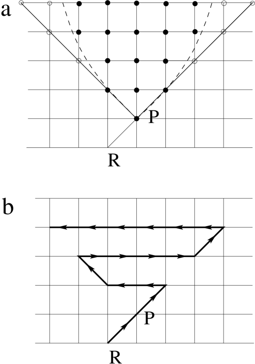
Figure 2:

Figure 3:

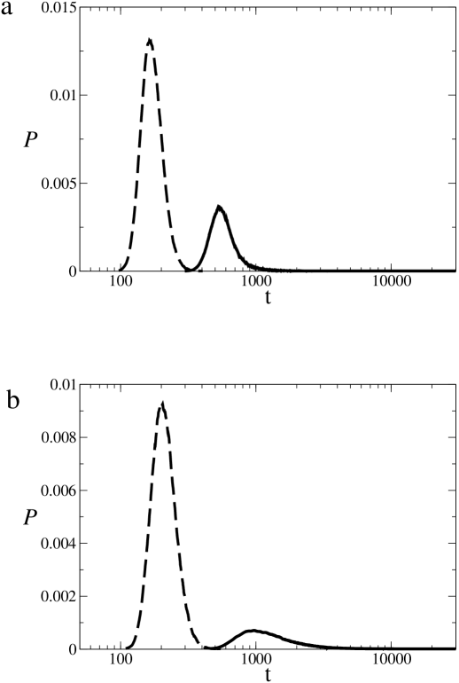
Figure 4:

References

- [1] Mechanism in Insect Olfaction, (1986), eds. Payne, T. L., Birch, M. C. & Kennedy M. C. (Oxford: Claredon).
- [2] Murlis, J., Elkinton, J. S. & Cardé, R. T. (1992) Annu. Rev. Entomol. 37, 505-32.
- [3] Malakoff, D. (2000) Science 286, 704-705.
- [4] Barinaga, M. (2000) Science 286, 705-706.
- [5] Weissburg, M. J., & Zimmer-Faust, R. K. (1994) J. Exp. Biol. 197, 349-375.
- [6] Atema, J. (1995) Proc. Natl. Acad. Sci. USA 92, 62-66.
- [7] Purcell, E. M. (1997). American Journal of Physics 45, 3-11.
- [8] Murlis, J. & Jones, C. D. (1981) Physiol. Entomol. 6, 71-86.
- [9] Murlis, J., Willis, M. A. & Cardé, R. T. (2000) Physiol. Entomol. 25, 211-222.
- [10] Tennekes, H. & Lumley, J. A first Course in Turbulence. (Cambridge, MA : MIT Press. 1972)
- [11] Shraiman, B. & Siggia, E. (2000) Nature 405, 639 - 646.
- [12] David, C. T. in Ref. [1], pp. 49-57.
- [13] Villermaux, E. & Innocenti, C. (1999) J. Fluid Mech. 393, 123-147.
- [14] Fackrell, J. E. & Robins, A. G. (1982) J. Fluid Mech. 117, 1-26.
- [15] Kennedy, J. S. in Ref. [1], pp. 11-25.
- [16] Baker, T. C. in Ref. [1], pp. 39-48.
- [17] David, C. T. Kennedy, J. S. & Ludlow, A. R. (1983) Nature 303.
- [18] Belanger, J. H. & Willis, M. A. (1996) Adapt. Behav. 4, 217-253.
- [19] Mafra-Neto, A. & Cardé, R. T. (1994) Nature 369, 142-144.
- [20] Kennedy, J. S., Ludlow, A. R. & Sanders, C. J. (1980) Nature 295, 475-477.
- [21] Taylor, J. I. (1921) Proc. London Math. Soc. 20, 196.
- [22] Duda, R. O. & Hart, P. E. Pattern Classification and Scene Analysis. (Wiley, New York, 1973).
- [23] Rozanov, Yu. A. Probability Theory, Random Processes & Mathematical Statistics (Kluwer Academic Publishers 1995).
- [24] Belanger, J. H. & Arbas, E. A. (1998) J. Comp. Physiol. A 183, 345-360.
- [25] Willis, M. A. & Arbas, E. A. (1998) J. Comp. Physiol. A 182, 191-202.
- [26] Consi, T. R., Grasso, F., Mountain, D. & Atema, J. (1995) The Biological Bulletin 189, 231-232.
- [27] Russel, R. A. Odor Detection by Mobile robots. (World Scientific, Singapore, 1999).
- [28] A. T. Hayes, A. Martinoli, and R. M. Goodman. (2000) In: Parker L., editor, Proc. of the Fifth Int. Symp. on Distributed Autonomous Robotic Systems, Knoxville, TN, October.
- [29] S. Kazadi, R. Goodman R. D. Tsikata, & Lin H. (2000) Autonomous Robots. 9 175-188.
- [30] Berg, H. (1990) Cold Spring Harbor Symp. Quant. Biol. 55, 539-545.
- [31] Devreotes, P.N. and Zigmond, S.H. (1988) Annu. Rev. Cell Biol., 4, 649-686, .
- [32] R. S. Sutton, A. G. Barto, Reinforcement Learning: An Introduction (MIT Press, Cambridge, MA, 1998.)