Energy transfer in two-dimensional magnetohydrodynamic turbulence: formalism and numerical results

Abstract

The basic entity of nonlinear interaction in Navier-Stokes and the Magnetohydrodynamic (MHD) equations is a wavenumber triad (k,p,q) satisfying ${\bf k+p+q=0}$. The expression for the combined energy transfer from two of these wavenumbers to the third wavenumber is known. In this paper we introduce the idea of an effective energy transfer between a pair of modes by the mediation of the third mode, and find an expression for it. Then we apply this formalism to compute the energy transfer in the quasi-steady-state of two-dimensional MHD turbulence with large-scale kinetic forcing. The computation of energy fluxes and the energy transfer between different wavenumber shells is done using the data generated by the pseudo-spectral direct numerical simulation. The picture of energy flux that emerges is quite complex—there is a forward cascade of magnetic energy, an inverse cascade of kinetic energy, a flux of energy from the kinetic to the magnetic field, and a reverse flux which transfers the energy back to the kinetic from the magnetic. The energy transfer between different wavenumber shells is also complex—local and nonlocal transfers often possess opposing features, i.e., energy transfer between some wavenumber shells occurs from kinetic to magnetic, and between other wavenumber shells this transfer is reversed. The net transfer of energy is from kinetic to magnetic. The results obtained from the studies of flux and shell-to-shell energy transfer are consistent with each other.

PACS: 47.65.+a,47.27-i,47.11.+j

I Introduction

In fluid and MHD turbulence, eddies of various sizes interact amongst themselves; energy is exchanged among them in this process. These interactions arise due to the nonlinearity present in these systems. The fundamental interactions involve wavenumber triads (k,p,q) satisfying ${\bf k+p+q=0}$. The combined energy transfer computation to a mode from the other two modes of a triad has generally been considered to be fundamental. This formalism has played an important role in furthering our understanding of interactions in fluid turbulence. In this paper we present a new scheme to calculate the energy transfer rate between two modes in a triad interaction in magnetohydrodynamic (MHD) turbulence—we call it the mode-to-mode transfer. Using our scheme we calculate cascade rates and energy transfer rates between two wavenumber shells.

The energy spectra and cascade rates are quantities of interest in the statistical theory of MHD turbulence. Recent numerical [1, 2, 3] and theoretical [4, 5, 6] work indicate that the energy spectrum of total energy is proportional to $k^{-5/3}$, similar to that found in fluid turbulence. Sridhar and Goldreich [7] and Goldreich and Sridhar [8] studied the energy spectrum in presence of strong magnetic field and found it to be proportional $k_{\perp}^{-5/3}$ ($k_{\perp}$ is the perpendicular component of the wavevector). Most of the work on MHD turbulence focus on the energy spectrum of either total energy or on the spectra of Elsässer variables (${\bf u\pm b}$, where u and b are velocity and magnetic fields respectively). In this paper we will focus on various energy cascade rates of MHD turbulence. The magnetic energy (denoted by ME) of a mode evolves due to two nonlinear terms, ${\bf[b.(u.\nabla)b]}$ and ${\bf[b.(b.\nabla)u]}$, of the MHD equations; the first term exchanges ME between different scales, and the second term exchanges magnetic and kinetic energy (denoted by KE) between different scales. The KE similarly evolves due to two nonlinear terms ${\bf[u.(u.\nabla)u]}$ and ${\bf[u.(b.\nabla)b]}$; the first one exchanges KE between different scales and the second exchanges energy between the magnetic and the velocity fields.

Pouquet et al. [9] studied the energy transfer between large and small scales using three-dimensional (3D) EDQNM closure calculations. For nonhelical MHD they argued that the ME cascades forward, i.e., from large scales to small scales. In presence of helicity, the large-scale magnetic field grows, which in turn brings equipartition the small-scale kinetic and magnetic energy by Alfvén effect. The residual helicity, the difference between kinetic and magnetic helicity , induces growth of large-scale magnetic energy and helicity. Pouquet and Patterson [10] arrived at a similar conclusion based on their numerical simulations. Their simulation results also indicated that magnetic helicity, not necessarily the residual helicity, is important for the growth of large-scale magnetic field. Earlier, Batchelor [11] had argued for transfer between kinetic and magnetic energies at small scales; his arguments were based on an analogy between the magnetic field equation of MHD and the vorticity equation.

In a 2D EDQNM study, Pouquet [12] obtained eddy viscosities for MHD turbulence. Upon injection of kinetic and magnetic energy, she obtained a quasi stationary-state with a direct cascade of energy to small scales together with an inverse cascade of mean-square magnetic vector potential. In the inverse cascade regime, she argued that the small-scale ME acts like a negative eddy viscosity on the large-scale ME. The inverse cascade of the mean-square magnetic vector potential was conjectured to arise due to the destablization of the large-scale magnetic field by the small-scale magnetic field. She also argued that the small-scale KE has the effect of a positive eddy viscosity on the large-scale ME. Ishizawa and Hattori [13] in their EDQNM calculation obtained the eddy viscosity due to each of the nonlinear terms in MHD equations. They found that the eddy viscosity due to ${\bf(b.\nabla)u}$ is positive, leading to a transfer of energy from large-scale magnetic field to small-scale magnetic field, apparently contradicting Pouquet’s work [12]. However, this discrepancy may be because Pouquet considers the regime of inverse cascade of mean-square vector potential, while Ishizawa and Hattori [13] calculation may capture the other wavenumber range. One of the similarities between Pouquet [12] and Ishizawa and Hattori’s [13] calculations is that both of them give a non-local energy transfer from small-scale velocity field to the large-scale velocity field. In a recent work Ishizawa and Hattori [14] employed the wavelet basis to investigate energy transfer in 2D MHD turbulence.

In this paper we have computed various cascade rates and other forms of energy transfers using 2D MHD simulations. It is in anticipation that some of the conclusion drawn here will shed light on the nature of interactions of both 2D and 3D MHD because the nature of cascade of the total energy is similar in 2D and 3D [15]. It is known that the ME decays in 2D MHD turbulence [16]. However, this decay occurs only after a finite time, during which the ME is steady. We have calculated our fluxes and shell-to-shell energy transfer rates for this “quasi steady state”. We must however add that the methods used here are completely generalizable to the 3D case. We have restricted ourselves to 2D purely because of unavailability of powerful computing resources to us.

Most of the earlier work on energy transfer in MHD turbulence (e.g., [9, 10]) often dealt mainly with coarse-grained energy transfer (between large scales and small scales). In a recent work, Frick and Sokoloff [17] solved a shell model of MHD turbulence and calculated only the KE flux between the velocity modes, and the ME flux between the magnetic modes. In our simulations we investigate energy transfer between u-to-u, b-to-b, and u-to-b modes. These results provide us with more informed picture of the physics of energy transfer in MHD turbulence.

The paper is organized as follows: In Section II we discuss the known results of energy transfer in a MHD triad, and introduce a new formalism called “mode-to-mode energy transfer”. Using the formalism of the mode-to-mode transfer, we derive in Section III the formulas for various energy fluxes and shell-to-shell energy transfer rates. The simulation methodology is discussed in Section IV. In Section V we report the numerically calculated energy fluxes and shell-to-shell transfer rates. The results are summarized in the last section. Appendix contains derivation of the formulas for the mode-to-mode transfer rates.

II Energy transfers in a MHD triad

We will first state the known result on the energy transfers in a triad. Then we will introduce a new formalism called “mode-to-mode” energy transfer in turbulence.

The incompressible MHD equations in real space are

$$\frac{\partial{\bf u}}{\partial t}+{\bf(u\cdot\nabla)u} = -\nabla p+{\bf(b\cdot\nabla)b}+\nu\nabla^{2}{\bf u}$$ (1)

$$\frac{\partial{\bf b}}{\partial t}+{\bf(u\cdot\nabla)b} = -{\bf(b\cdot\nabla)u}+\eta\nabla^{2}{\bf b}$$ (2)

$$\nabla\cdot{\bf u} = 0$$ (3)

$$\nabla\cdot{\bf b} = 0$$ (4)

where ${\bf u}$ and ${\bf b}$ are the velocity and magnetic fields respectively, $p$ is the total pressure, and $\nu$ and $\eta$ are the kinematic viscosity and magnetic diffusivity respectively. We have assumed that the mean magnetic field is zero. In Fourier space, the KE ($E^{u}({\bf k})={\bf|u(k)|}^{2}/2$) and the ME ($E^{b}({\bf k})={\bf|b(k)|}^{2}/2$) evolution equations are [9, 18, 19]

$$\frac{\partial E^{u}(\bf k)}{\partial t}+2\nu k^{2}E^{u}({\bf k}) = \sum_{{\bf k+p+q}=0}\frac{1}{2}S^{uu}({\bf k|p,q})+\sum_{{\bf k+p+q}=0}\frac{1}{2}S^{ub}({\bf k|p,q})$$ (5)

$$\frac{\partial E^{b}(\bf k)}{\partial t}+2\eta k^{2}E^{b}({\bf k}) = \sum_{{\bf k+p+q}=0}\frac{1}{2}S^{bb}({\bf k|p,q})+\sum_{{\bf k+p+q}=0}\frac{1}{2}S^{bu}({\bf k|p,q})$$ (6)

The four nonlinear terms $S^{uu}({\bf k|p,q})$, $S^{ub}({\bf k|p,q})$, $S^{bb}({\bf k|p,q})$, and $S^{bu}({\bf k|p,q})$ are

$$S^{uu}({\bf k|p,q}) = {{S\hskip-6.70831pt\hbox to6.70831pt{\hss\sl/\/\hss}}}^{uu}({\bf k|p|q})+{{S\hskip-6.70831pt\hbox to6.70831pt{\hss\sl/\/\hss}}}^{uu}({\bf k|q|p})$$ (7)

$$S^{bb}({\bf k|p,q}) = {\cal{S\hskip-6.70831pt\hbox to6.70831pt{\hss\sl/\/\hss}}}^{bb}({\bf k|p|q})+{\cal{S\hskip-6.70831pt\hbox to6.70831pt{\hss\sl/\/\hss}}}^{bb}({\bf k|q|p})$$ (8)

$$S^{ub}({\bf k|p,q}) = {\cal{S\hskip-6.70831pt\hbox to6.70831pt{\hss\sl/\/\hss}}}^{ub}({\bf k|p|q})+{\cal{S\hskip-6.70831pt\hbox to6.70831pt{\hss\sl/\/\hss}}}^{ub}({\bf k|q|p})$$ (9)

$$S^{bu}({\bf k|p,q}) = {\cal{S\hskip-6.70831pt\hbox to6.70831pt{\hss\sl/\/\hss}}}^{bu}({\bf k|p|q})+{\cal{S\hskip-6.70831pt\hbox to6.70831pt{\hss\sl/\/\hss}}}^{bu}({\bf k|q|p})$$ (10)

where

$${\cal{S\hskip-6.70831pt\hbox to6.70831pt{\hss\sl/\/\hss}}}^{uu}({\bf k|p|q}) = -\Im({\bf[k.u(q)][u(k).u(p)]})$$ (11)

$${\cal{S\hskip-6.70831pt\hbox to6.70831pt{\hss\sl/\/\hss}}}^{bb}({\bf k|p|q}) = -\Im({\bf[k.u(q)][b(k).b(p)]})$$ (12)

$${\cal{S\hskip-6.70831pt\hbox to6.70831pt{\hss\sl/\/\hss}}}^{ub}({\bf k|p|q}) = \Im({\bf[k.b(q)][u(k).b(p)]})$$ (13)

$${\cal{S\hskip-6.70831pt\hbox to6.70831pt{\hss\sl/\/\hss}}}^{bu}({\bf k|p|q}) = \Im({\bf[k.b(q)][b(k).u(p)]})$$ (14)

where $\Im$ stands for the imaginary part of the argument.

The terms $S^{\beta\alpha}({\bf k|p,q})$, where $\alpha,\beta$ stand for $u$ or $b$, are conventionally taken to represent the nonlinear energy transfer from modes ${\bf p}$ and ${\bf q}$ to mode ${\bf k}$ [9, 18, 19]. In the following discussion we derive a more detailed expression to obtain the energy transfer between any two modes within a triad; we will refer to this as the “mode-to-mode transfer”. We emphasize that this approach is still within the framework of the triad interaction, i.e., the triad is still the fundamental entity of interaction of which the mode-to-mode energy transfer is a part. An expression for the energy transfer between two modes of a triad by the mediation of the third mode is sought here.

Suppose in the triad (${\bf k,p,q}$), ${\cal{R\hskip-7.67015pt\hbox to7.67015pt{\hss\sl/\/\hss}}}^{uu}({\bf k|p|q})$ denotes the KE transfer from mode ${\bf p}$ to mode ${\bf k}$ with mode ${\bf q}$ as a mediator, and ${\cal{R\hskip-7.67015pt\hbox to7.67015pt{\hss\sl/\/\hss}}}^{uu}({\bf k|q|p})$ denotes the KE transfer from mode ${\bf q}$ to mode ${\bf k}$ with ${\bf p}$ as a mediator, then by definition,

$${\cal{R\hskip-7.67015pt\hbox to7.67015pt{\hss\sl/\/\hss}}}^{uu}({\bf k|p|q})+{\cal{R\hskip-7.67015pt\hbox to7.67015pt{\hss\sl/\/\hss}}}^{uu}({\bf k|q|p})=S^{uu}({\bf k|p,q}).$$ (15)

In addition, the energy transfer from u(k) to u(p), ${\cal{R\hskip-7.67015pt\hbox to7.67015pt{\hss\sl/\/\hss}}}^{uu}({\bf k|p|q})$, should be equal and opposite to the transfer from u(p) to u(k), ${\cal{R\hskip-7.67015pt\hbox to7.67015pt{\hss\sl/\/\hss}}}^{uu}({\bf p|k|q})$, that is,

$${\cal{R\hskip-7.67015pt\hbox to7.67015pt{\hss\sl/\/\hss}}}^{bb}({\bf k|p|q})+{\cal{R\hskip-7.67015pt\hbox to7.67015pt{\hss\sl/\/\hss}}}^{bb}({\bf p|k|q})=0.$$ (16)

Similar equations can be written for other pair of modes, and also for $b$-to-$b$ and $u$-to-$b$ transfer (see Fig. 1). Our objective is to obtain an expression for ${\cal{R\hskip-7.67015pt\hbox to7.67015pt{\hss\sl/\/\hss}}}^{\beta\alpha}({\bf k|p|q})$ in terms of ${\bf k,p,q,u(k),u(p),u(q),b(k),b(p),b(q)}$.

It is shown in the Appendix that ${\cal{R\hskip-7.67015pt\hbox to7.67015pt{\hss\sl/\/\hss}}}^{uu}({\bf k|p|q})={\cal{S\hskip-6.70831pt\hbox to6.70831pt{\hss\sl/\/\hss}}}^{uu}({\bf k|p|q})+X_{\Delta}$; ${\cal{R\hskip-7.67015pt\hbox to7.67015pt{\hss\sl/\/\hss}}}^{bb}({\bf k|p|q})={\cal{S\hskip-6.70831pt\hbox to6.70831pt{\hss\sl/\/\hss}}}^{bb}({\bf k|p|q})+Y_{\Delta}$, and ${\cal{R\hskip-7.67015pt\hbox to7.67015pt{\hss\sl/\/\hss}}}^{bu}({\bf k|p|q})={\cal{S\hskip-6.70831pt\hbox to6.70831pt{\hss\sl/\/\hss}}}^{bu}({\bf k|p|q})+X_{\Delta}$, where ${\cal{S\hskip-6.70831pt\hbox to6.70831pt{\hss\sl/\/\hss}}}^{\beta\alpha}({\bf k|p|q})$s are given by Eq. (11-14). In Fig. 2 we illustrate all these mode-to-mode transfers ${\cal{R\hskip-7.67015pt\hbox to7.67015pt{\hss\sl/\/\hss}}}^{\alpha\beta}({\bf k|p|q})$. The constants $X_{\Delta},Y_{\Delta},Z_{\Delta}$ have special significance, and are described below.

We take KE transfer rate as an example. In Fig. 2 we observe that ${\cal{S\hskip-6.70831pt\hbox to6.70831pt{\hss\sl/\/\hss}}}^{uu}({\bf k|p|q})+X_{\Delta}$ gets transferred from u(p) to u(k), ${\cal{S\hskip-6.70831pt\hbox to6.70831pt{\hss\sl/\/\hss}}}^{uu}({\bf q|k|p})+X_{\Delta}$ gets transferred from u(k) to u(q), and ${\cal{S\hskip-6.70831pt\hbox to6.70831pt{\hss\sl/\/\hss}}}^{uu}({\bf p|q|k})+X_{\Delta}$ gets transferred from u(q) to u(p). The quantity $X_{\Delta}$ flows along ${\bf u(p)}\rightarrow{\bf u(k)}\rightarrow{\bf u(q)}\rightarrow{\bf u(p)}$, circulating around the entire triad without changing the energy of any of the velocity modes. Therefore we will call it the “circulating transfer”. The circulating transfer lost by a mode is regained, hence, this term does not affect the overall energy input/output of a mode. Therefore ${\cal{S\hskip-6.70831pt\hbox to6.70831pt{\hss\sl/\/\hss}}}^{uu}({\bf k|p|q})$ [cf. Eq. (11)] is the only term which effectively participates in the energy transfer. That is why it is termed as the “effective mode-to-mode transfer rate” from mode u(p) to mode u(k), mediated by mode u(q). There are two other circulating transfers: $Y_{\Delta}$ for $b$-to-$b$ transfer, and $Z_{\Delta}$ for $u$-to-$b$ transfer; they are illustrated in Fig. 2. A derivation of the effective mode-to-mode transfer is given in Appendix. For further details, refer to Ph. D. thesis of Dar [20] and Dar et al. [21].

In summary, we have obtained a formula for “effective mode-to-mode energy transfer rates” in MHD turbulence. The effective KE transfer rates from mode ${\bf p}$ to ${\bf k}$ is ${\cal{S\hskip-6.70831pt\hbox to6.70831pt{\hss\sl/\/\hss}}}^{uu}({\bf k|p|q})$, the effective ME transfer rates from mode ${\bf p}$ to ${\bf k}$ is ${\cal{S\hskip-6.70831pt\hbox to6.70831pt{\hss\sl/\/\hss}}}^{bb}({\bf k|p|q})$, and the effective “conversion” rate of KE of mode ${\bf p}$ to ME of mode ${\bf k}$ is ${\cal{S\hskip-6.70831pt\hbox to6.70831pt{\hss\sl/\/\hss}}}^{bu}({\bf k|p|q})$. The rate ${\cal{S\hskip-6.70831pt\hbox to6.70831pt{\hss\sl/\/\hss}}}^{bu}({\bf k|p|q})$ is responsible for the growth of magnetic energy. In all these effective energy transfers, the mode with wavenumber ${\bf q}$ mediates the transfer.

In the next section we will use our “effective mode-to-mode energy transfer rate” formalism to derive formulas for cascade rates and shell-to-shell energy transfer.

III Cascade rates and Shell-to-Shell energy transfer in MHD turbulence

In this section we will use the formalism of effective mode-to-mode transfers to define cascade rates and shell-to-shell energy transfer rates in MHD turbulence. Note that the formulas for cascade rate etc. derived using our mode-to-mode transfer is equivalent to those derive with $S(k|p,q)$. However, our formalism has certain advantages. For example, some of the cascade rates and shell-to-shell transfers (defined below) which were not accessible with the earlier formalisms can now be calculated using our scheme. In addition, the flux and shell-to-shell transfer formulas using our schemes are simpler. In this paper we shall use the term u-sphere (shell) to denote a sphere (shell) wavenumber-space containing velocity modes. Similarly, the b-sphere (shell) denote the corresponding sphere (shell) of magnetic modes.

A Energy cascade rates

The energy cascade rate (or flux) is defined as the rate of loss of energy from a sphere in the wavenumber space to the modes outside. There are various types of cascade rates in MHD turbulence. We have schematically shown these transfers in Fig. 3. The energy transfer could take take place from inside/outside $u/b$-sphere to inside/outside-$u/b$ sphere. In terms of ${\cal{S\hskip-6.70831pt\hbox to6.70831pt{\hss\sl/\/\hss}}}^{\alpha\beta}({\bf k|p|q})$, the energy cascade rate from inside of the $\alpha$-sphere of radius $K$ to outside of the $\beta$-sphere of the same radius is

$$\Pi^{\alpha<}_{\beta>}(K)=\sum_{|{\bf k}|>K}\sum_{|{\bf p}|<K}{\cal{S\hskip-6.70831pt\hbox to6.70831pt{\hss\sl/\/\hss}}}^{\beta\alpha}({\bf k|p|q}).$$ (17)

where $\alpha$ and $\beta$ stand for $u$ or $b$.

There is a transfer of energy from a u-sphere of radius $K$ to the b-sphere of the same radius. We can obtain the effective flux from the u-sphere to the b-sphere using

$$\Pi^{u<}_{b<}(K)=\sum_{|{\bf p}|<K}\sum_{|{\bf k}|<K}{\cal{S\hskip-6.70831pt\hbox to6.70831pt{\hss\sl/\/\hss}}}^{bu}({\bf k|p|q}).$$ (18)

Similarly, the energy flux from modes outside of the u-sphere to the modes outside of the b-sphere can be obtained by

$$\Pi^{u>}_{b>}(K)=\sum_{|{\bf p}|>K}\sum_{|{\bf k}|>K}{\cal{S\hskip-6.70831pt\hbox to6.70831pt{\hss\sl/\/\hss}}}^{bu}({\bf k|p|q}).$$ (19)

The total effective flux is defined as the total energy (kinetic+magnetic) lost by the $K$-sphere to the modes outside, i.e.,

$$\Pi_{tot}(K)=\Pi^{u<}_{u>}(K)+\Pi^{b<}_{b>}(K)+\Pi^{u<}_{b>}(K)+\Pi^{b<}_{u>}(K).$$ (20)

A schematic illustration of the effective fluxes defined in Eqs. (17)-(19) is shown in Fig. 3. In Section V B we will present the values of these fluxes calculated using numerical simulations of 2D MHD turbulence.

B Shell-to-Shell energy transfer rates

In this section we derive an expression for the energy transfer rates between two shells. Consider KE exchange between shell m and shell n shown in Fig. 4. For the triads shown in the figure, the mode k is in shell m, the mode p is in shell n, and mode q could be inside or outside the shells. In terms of the mode-to-mode transfer ${\cal{R\hskip-7.67015pt\hbox to7.67015pt{\hss\sl/\/\hss}}}^{uu}({\bf k|p|q})$, the rate of energy transfer from the $n^{th}$ $u$-shell to the $m^{th}$ $u$-shell is defined as

$$T^{uu}_{mn}=\sum_{{\bf k}{\epsilon}{\it m}}\sum_{{\bf p}{\epsilon{\it n}}}{\cal{R\hskip-7.67015pt\hbox to7.67015pt{\hss\sl/\/\hss}}}^{uu}({\bf k|p|q})$$ (21)

where the k-sum is over u-shell m and the p-sum is over u-shell n with k+p+q=0. As discussed in the last section, the quantity ${\cal{R\hskip-7.67015pt\hbox to7.67015pt{\hss\sl/\/\hss}}}^{uu}$ can be written as a sum of an effective transfer ${\cal{S\hskip-6.70831pt\hbox to6.70831pt{\hss\sl/\/\hss}}}^{uu}({\bf k|p|q})$ and a circulating transfer $X_{\Delta}$. We know from the last section that the circulating transfer does not contribute to the energy change of modes. From Fig. 4 we can see that $X_{\Delta}$ flows from shell m to shell n and then flows back to m indirectly through the mode q. Therefore the effective energy transfer rate from $n^{th}$ $u$-shell to $m^{th}$ $u$-shell is

$$T^{uu}_{mn}=\sum_{{\bf k}{\epsilon}{\it m}}\sum_{{\bf p}{\epsilon{\it n}}}{\cal{S\hskip-6.70831pt\hbox to6.70831pt{\hss\sl/\/\hss}}}^{uu}({\bf k|p|q}).$$ (22)

A general formula for shell-to-shell transfer from $m^{th}$ $\alpha$-shell to $n^{th}$ $\beta$-shell is

$$T^{\beta\alpha}_{mn}=\sum_{{\bf k}{\epsilon}{\it m}}\sum_{{\bf p}{\epsilon{\it n}}}{\cal{S\hskip-6.70831pt\hbox to6.70831pt{\hss\sl/\/\hss}}}^{\beta\alpha}({\bf k|p|q}),$$ (23)

Earlier Domaradzki and Rogallo [22] had given the following formula for shell-to-shell energy transfer in terms of $S^{uu}({\bf k|p,q})$:

$$T^{uu}_{mn}=\frac{1}{2}\sum_{{\bf k}{\epsilon}{\it m}}\sum_{{\bf p}{\epsilon{\it n}}}S^{uu}({\bf k|p,q}).$$ (24)

This formula is incorrect due to the following reasons. The formula (24) has contributions from two types of wavenumber triads (see Fig. 4). In both the triads, the wavenumber ${\bf k}$ is located in the shell $m$. However, Type I triads have both wavenumbers ${\bf p,q}$ in the shell $n$, but Type II triads have only wavenumber ${\bf p}$ in the shell $n$. Clearly, to compute the energy transfer from shell $n$ to shell $m$, we must include all the triad interactions of type I, but only the mode p to mode k energy transfer of type II triads. Inclusion of mode q to mode k will lead to incorrect estimation. This is the drawback of Domaradzki and Rogallo’s formalism. The above inconsistency has been hinted at by Batchelor [11] and Domaradzki and Rogallo [22] themselves.

In summary, Batchelor’s and Domaradzki and Rogallo’s formalism does not yield correct shell-to-shell energy transfers; we have used an alternate formula [Eq. (23)] to compute them. We have numerically computed them using the numerical data of 2D MHD turbulence. These results, discussed in Section  V C, provide important insights into the energy transfer process in MHD turbulence.

IV Simulation Details

A Numerical Method

In our simulations we use the Elsässer variable ${\bf z}^{\pm}={\bf u}\pm{\bf b}$ instead of u and b. The MHD equations (1) and (2) written in terms of ${\bf z}^{+}$ and ${\bf z}^{-}$ are

$$\frac{\partial{\bf z}^{\pm}}{\partial{t}}+\left({\bf z}^{\mp}\cdot{\bf\nabla}\right){\bf z}^{\pm} = -{\bf\nabla}p+\nu_{\pm}\nabla^{2}{\bf z}^{\pm}+\nu_{\mp}\nabla^{2}{\bf z}^{\mp}$$ (26)

$$+\left(\nu_{\pm}/k_{eq}^{2}\right)\nabla^{4}{\bf z}^{\pm}+\left(\nu_{\mp}/k_{eq}^{2}\right)\nabla^{4}{\bf z}^{\mp}+{\bf F^{\pm}}$$

where $\nu_{\pm}=(\nu\pm\eta)/2$. In addition to the viscosity and the magnetic diffusivity of Eqs. (1) and (2), Eq. (26) includes hyperviscosity ($\nu_{\pm}/k_{eq}^{2}$) to damp out the energy at very high wavenumbers. We choose $\nu=\eta=5\times 10^{-6}$ for runs on a grid of size $512\times 512$. The parameter $k_{eq}$ is chosen to be 14 for all the runs. The terms ${\bf F^{\pm}}$ are the forcing functions. The corresponding forcing functions for the $\bf u$ and the $\bf b$ fields in terms of ${\bf F^{\pm}}$ will be ${\bf F}^{u}=({\bf F}^{+}+{\bf F}^{-})/2$ and ${\bf F}^{b}=({\bf F}^{+}-{\bf F}^{-})/2$. In our simulations, we do not force the magnetic field (i.e, ${\bf F}^{b}=0$). Consequently, we get ${\bf F}^{+}={\bf F}^{-}={\bf F}^{u}={\bf F}$. The absence of magnetic forcing is motivated by the dynamo (magnetic field amplification) calculations where only KE is forced. Some of the physical examples where only KE is forced are galactic dynamo and earth’s magnetic field generation. Even though our simulations are two-dimensional, we have followed the similar line of approach as the dynamo simulations.

We use the pseudo-spectral method [23] to solve the above equations in a periodic box of size $2\pi\times 2\pi$. In order to remove the aliasing errors arising in the pseudo-spectral method a square truncation is performed wherein all the modes with $|k_{x}|\geq N/3$ or $|k_{y}|\geq N/3$ $(N=512)$ are set equal to zero. The equations are time advanced using the second order Adam-Bashforth scheme for the convective term and the Crank-Nicholson scheme for the viscous terms. The time step $\Delta t$ used for these runs is $5\times 10^{-4}$. All the quantities are non-dimensionalised using the initial total energy (one unit) and length scale of $2\pi$. Normalized cross-helicity, defined as

$$\sigma_{c}=\frac{2\int{\bf u.b}d^{3}x}{\int(u^{2}+b^{2})d^{3}x)},$$ (27)

has the value approximately equal to 0.1 for the results discussed in the paper. However, we have carried out simulations up-to $\sigma_{c}\approx 0.9$ and the results obtained for the higher $\sigma_{c}$’s were found to be qualitatively similar to those discussed in this paper.

At each time step we construct $\bf F$ as a divergenceless uncorrelated random function (${\bf\nabla.F}=0$). The $x$-component of $\bf F$ is determined at every time step by

$$F_{x}=\left(\frac{k_{y}}{k}\right)\sqrt{\Delta t}{\cal F}e^{i\phi},$$ (28)

where ${\cal F}^{2}$ is equal to the average energy input rate per mode, and phase $\phi$ is a uniformly distributed random variable between $0$ and $2\pi$. The $y$-component of the forcing function is obtained by using the divergenceless condition, which yields

$$F_{y}=-\left(\frac{k_{x}}{k_{y}}\right)F_{x}.$$ (29)

We apply isotropic forcing over a wavenumber annulus $4<k<5$. The value of ${\cal F}^{2}$ is determined from the average rate of the total energy input, which in our simulation is chosen to be equal to 0.1.

B Numerical computation of fluxes

To compute the fluxes we employ a method similar to that used by Domaradzki and Rogallo [22]. We outline this method below using $\Pi^{b<}_{u>}(K)$ as an example. In Eq. (17) we substitute the expression for ${\cal{S\hskip-6.70831pt\hbox to6.70831pt{\hss\sl/\/\hss}}}^{ub}(k|p|q)$ from Eq. (13) :

$$\Pi^{b<}_{u>}(K)=\sum_{|{\bf k}|>K}\sum_{|{\bf p}|<K}\Im\left({\bf\left[k.b(q)\right]}{\bf\left[u(k).b(p)\right]}\right)$$ (30)

A straightforward summation over k and p involves $O(N^{2})$ ($N$ = grid size) operations, and would thus involve a prohibitive computational cost for large $N$ simulations. Instead, the pseudo-spectral method can be used to compute the above flux in $O(NlogN)$ operations. The procedure is as follows:

We define two “truncated” variables ${\bf u}^{>}$ and ${\bf b}^{<}$ as follows

$${\bf u}^{>}({\bf k})=\left\{\begin{array}[]{ll}0&\mbox{if $|{\bf k}|<K$}\\ {\bf u}({\bf k})&\mbox{if $|{\bf k}|>K$}\end{array}\right.$$ (31)

and

$${\bf b}^{<}({\bf p})=\left\{\begin{array}[]{ll}{\bf b}({\bf p})&\mbox{if $|{\bf p}|<K$}\\ 0&\mbox{if $|{\bf p}|>K$}\end{array}\right.$$ (32)

Eq. (30) written in terms of ${\bf u}^{>}$ and ${\bf b}^{<}$ reads as follows

$$\Pi^{b<}_{u>}(K)=\sum_{\bf k}\sum_{\bf p}\Im\left({\bf\left[k.b(k-p)\right]}{\bf\left[u^{>}(k).b^{<}(p)\right]}\right).$$ (33)

The above equation may be written as

$$\Pi^{b<}_{u>}(K)=\Im\left[\sum_{\bf k}k_{j}u_{i}^{>}({\bf k})\sum_{\bf p}b_{j}({\bf k-p})b_{i}^{<}({\bf p})\right]$$ (34)

The ${\bf p}$ summation in the above equation can be recognized as a convolution sum. The right hand side of Eq. (34) can be efficiently evaluated by the pseudo-spectral method using the truncated variables ${\bf u}^{>}$ and ${\bf b}^{<}$. This procedure has to be repeated for every value of $K$ for which the flux needs to be computed. The rest of the fluxes and transfer rates defined in Section III are similarly computed.

In the following section we describe the results of our simulations.

V Simulation Results

A Generation of Steady State

We compute the fluxes and the shell-to-shell transfers for steady state. However, the computational time required to obtain a statistically steady state on a grid of size $512^{2}$ is large. So to obtain a steady state in simulations on this grid, we proceed in stages. First, we run on a grid of size $64^{2}$ till a steady state is achieved. This steady state field is then used as the initial condition to achieve a steady-state for $128^{2}$, and similarly to the grid of sizes $256^{2}$ and $512^{2}$.

Theoretically, the magnetic energy in two-dimensional MHD decays in the long run even with steady KE forcing [16]. However, we find that the ME remains steady for sufficiently long time before it starts to decay. For $128^{2}$ simulation, the decay of ME starts only after $t=25-30$ time units, and for $512^{2}$, the decay starts much later. We term this region of constant ME as “quasi steady-state”. In Fig. 5 we show both KE and ME for this state. Here the Alfvén ratio (KE/ME) fluctuates between the values $0.4$ and $0.56$, hence ME dominates KE. The flux and the shell-to-shell transfer rates reported in this paper is averaged over this quasi steady-state. The averaging is done once in every unit of non-dimensional time over 15 time units. The averaged spectra of KE and ME over this period is shown in Fig. 6. For the intermediate range of wavenumbers (inertial range), the spectra show a powerlaw behaviour. The spectral indices are in the range of 1.5-1.7, hence the determination of MHD spectral index is quite difficult. However, from the flux studies, Verma et al. [1] had concluded that Kolmogorov’s $5/3$ exponent is preferred over Kraichnan’s $3/2$ exponent. Müller and Biskamp [2] and Biskamp and Müller arrived at a similar conclusion based on their high resolution simulation.

B Flux studies

We compute all the energy fluxes defined in subsection III A by averaging over the outputs of our numerical simulation. In Fig. 7 we show all the fluxes. The total flux $\Pi_{tot}$ is positive indicating that there is a net loss of energy from the $K$-sphere to modes outside. In the wavenumber region $25<K<50$, the total flux is approximately constant. This wavenumber region is the inertial range.

The net transfer from KE to ME is a sum of the fluxes $\Pi^{u<}_{b<}(K)$, $\Pi^{u<}_{b>}(K)$, $\Pi^{u>}_{b<}$, and $\Pi^{u>}_{b>}(K)$. We observe from Fig. 7 that the fluxes $\Pi^{u<}_{b>}(K_{max})$, $\Pi^{u>}_{b<}(K_{max})$ and $\Pi^{u>}_{b>}(K_{max})$ are zero, understandably so because there is no mode outside this sphere of maximum radius $K_{max}$. The flux $\Pi^{u<}_{b<}(K_{max})$ is found to be positive, indicating that there is a net transfer from kinetic energy to magnetic energy.

We remind the reader that the u-modes within a wavenumber sphere are called the u-sphere, and the b-modes within the wavenumber sphere are called the b-sphere. We find that the flux $\Pi^{u<}_{b<}(K)$ is positive—hence, KE is lost by a u-sphere to the corresponding b-sphere. The flux $\Pi^{u<}_{b>}(K)$ is also positive. It means that a u-sphere loses energy to the modes outside the b-sphere. We find that the flux $\Pi^{b<}_{u>}(K)$ is negative, which implies that the b-sphere gains energy from modes outside the u-sphere. Thus, all these fluxes result in a transfer of KE to ME. However, $\Pi^{u>}_{b>}(K)$ is negative, implying that there is some feedback of energy from modes outside the b-sphere to modes outside the u-sphere. The net transfer, however, is from KE to ME. We shall later show that the flux $\Pi^{u>}_{b>}(K)$ plays a crucial role in driving the kinetic-to-kinetic flux $\Pi^{u<}_{u>}(K)$.

The energy gained by the b-spheres is found to be approximately constant for the range $20\leq K\leq K_{max}$. This can be seen from the plot of $\Pi^{b<}_{u<}(K)+\Pi^{b<}_{u>}$. The constancy of the flux implies that a b-sphere of radius $K$ and that of radius of $K+\Delta K$ get the same amount of energy from the u-modes. Thus there is no net energy transfer from the u-modes into a b-shell (of thickness $\Delta K$) of the inertial range. We therefore conclude that the net energy transfer from u-modes to the b-sphere occurs within the $K\leq 20$ sphere (the large length scales).

We find that the flux $\Pi^{u<}_{u>}(K)$ is negative, that is the inertial range u-sphere gain energy from the outside u-modes—this is consistent with the numerical simulations of Ishizawa and Hattori [14]. This behaviour of kinetic energy is known as an “inverse cascade” in literature and is reminiscent of the inverse cascade of KE in 2D fluid turbulence [19] and of mean square vector potential in 2D MHD turbulence [12]. Note, however that the KE in 2D MHD turbulence is not an inviscid invariant. Fig. 7 shows that the inverse cascade of kinetic energy exists in the wavenumber range $K\leq 60$. Even the modes that are being forced ($4\leq k\leq 5$) gain energy from higher wavenumbers u-modes. The source of this energy is the positive flux $\Pi^{b>}_{u>}(K)$ from higher b-modes to the higher u-modes.

We also observe from Fig. 7 that there is a loss of magnetic energy from the b-sphere to the b-modes outside [see $\Pi^{b<}_{b>}(K)$], i.e., the ME cascade is forward. This result is consistent with the numerical results of Ishizawa and Hattori [14]. The flux $\Pi^{b<}_{b>}(K)$ is found to be constant in the inertial range. Using similar reasoning to that given above, we can again conclude that the net magnetic energy transfer to a wavenumber shell in the inertial range is zero.

The above mentioned results are schematically illustrates in Fig. 8 for an inertial range wavenumber $K=20$. The energy input due to forcing and the small inverse cascade [$\Pi^{u<}_{u>}(K)$] into the u-sphere from higher u-modes provides the energy input into the u-sphere. This energy is transferred into and outside the b-sphere by $\Pi^{u<}_{b<}(K)$ and $\Pi^{u<}_{b>}(K)$ respectively, the latter transfer being the most significant of all transfers. The energy transferred into the b-sphere from the u-sphere [$\Pi^{u<}_{b<}(K)$] and a small input from the modes outside the u-sphere [$-\Pi^{b<}_{u>}(K)$] cascades down to the higher wavenumber b-modes. In the high wavenumber b-modes, the cascaded energy [$\Pi^{b<}_{b>}(K)$] and the energy transferred from the u-sphere are partly dissipated and partly fed back to the high wavenumber u-modes [$\Pi^{b>}_{u>}(K)$]. The feedback to the kinetic energy is mostly dissipated, but a small inverse cascade takes some energy back into the u-sphere. This is the qualitative picture of the energy transfer in 2D MHD turbulence.

The net transfer to each of the four corners of the Fig. 8 sum to zero within the statistical error (which is computed from the standard deviation of the sampled data). This is consistent with a quasi-steady-state picture. The results presented here for the quasi-steady-state in a forced turbulence remain qualitatively valid even for a decaying case—the direction of the various fluxes for the decaying case are identical to that for the forced simulation; but as the energy decays, the magnitudes of all the fluxes decrease.

The fluxes give us information about the overall energy transfer from inside/outside $u/b$-sphere to inside/outside $u/b$-sphere. To obtain a more detailed account of the energy transfer, energy exchange between the wavenumber shells have been studied; these results are presented in the next subsection.

C Shell-to-Shell energy transfer-rate studies

Significant details of energy transfers are revealed by calculating the shell-to-shell energy transfer rates $T^{\beta\alpha}_{mn}$ defined by Eq. (23). We partition the k-space into shells at wavenumbers $k_{n}(n=1,2,3,...)=1,16,19.02,22.62,...,2^{(n+14)/4}$. The first shell extends from $k_{1}=1$ to $k_{2}=16$, the second shell extends from $k_{2}=16$ to $k_{3}=19.02$, …, the $m^{th}$ shell extends from $k_{m}$ to $k_{(m+1)}$. Thus, the effective shell-to-shell energy transfer rate from the $n^{th}{\it\alpha}$-shell to the $m^{th}{\it\beta}$-shell [Eq. (23)] can be written as

$$T^{\beta\alpha}_{mn}=\sum_{k_{m}<k<k_{m+1}}\sum_{k_{n}<p<k_{n+1}}\sum_{\bf q}^{\Delta}{\cal{S\hskip-6.70831pt\hbox to6.70831pt{\hss\sl/\/\hss}}}^{\beta\alpha}({\bf k|p|q}).$$ (35)

The energy transfers ($u-u$, $b-b$, and $u-b$) involving shells which are close in wavenumber space are called local transfers, as is the convention. Two shells are considered close if the wavenumber ratio of the larger shell to the smaller shell is less than 2 (in this study this would include the shells between $n+4$ to $n-4$ for the $n$th shell). Transfers involving shells more distant than the above range are called non-local. Since two fields are involved in MHD, there are energy transfers between shells of same index. In the following discussions we will show that the energy transfer between $u$ and $b$ shells of same index plays a major role in MHD.

In Figs. 9, 10, and 11 we plot the energy transfer rates $T^{bb}_{mn},T^{uu}_{mn}$ and $T^{bu}_{mn}$ vs. $m$ respectively for various values of $n$. It is evident from the figures that the transfer rates between shells in the inertial range are virtually independent of the individual values of the indices $m$ and $n$, and only dependent on their differences. This means that the transfer rates in the inertial range are self-similar. The differences in $T^{\beta\alpha}_{mn}$ for various $n$ are smaller than the standard deviation of the sampled data, indicating that the perceived self-similarity is statistically significant.

In $T^{bb}_{mn}$ versus $m$ plot of Fig. 9 we find that the transfer rates $T^{bb}_{mn}$ are negative for $m<n$ and they are positive for $m>n$. Hence a b-shell gains energy from the b-shells of smaller wavenumbers and loses energy to the b-shells of larger wavenumbers. Hence, ME cascades from the smaller wavenumbers to the higher wavenumbers (forward). Since $T^{bb}_{mn}$ is self-similar, the energy lost from a shell ($n-\Delta n$) to $n$ is equal to the energy lost from $n$ to the shell ($n+\Delta n$). Thus, the net magnetic energy transfer into any inertial range shell is zero. In addition, we find that the most significant energy transfer takes place among $n-1,n$ and $n+1$ shells. Hence, $b-b$ energy transfer is local.

In $T^{uu}_{mn}$ versus $m$ of Fig. 10 we find that the most dominant transfers are from the $n^{th}$ u-shell to $(m=n\pm 1)^{th}$ shells. From the sign of these transfers we see that KE is gained from $(n-1)^{th}$ shell and lost to $(n+1)^{th}$ shell. This means that the local transfers from the adjacent shells result in a forward cascade of KE towards the large wavenumbers. The transfers from other shells are largely negligible except for the transfer to the shell $m=1$ (shown boxed on the left of the figure), which represents a loss of KE from high wavenumber modes to the $m=1$ shell. This nonlocal transfer (to the first shell) produces an inverse cascade of KE to the small wavenumbers, observed earlier in Section V B. Thus $u-u$ energy transfer has a forward energy cascade involving local interactions, and an inverse cascade involving nonlocal interactions with the first $u$-shell. The latter dominates the former in 2D turbulence.

We now discuss our simulation results for the energy transfer rates between u-shells and b-shells. In Fig. 11 we find that $T^{bu}_{mn}$ is positive for all $m$, except for $m=n-1$ and $n$. This implies that the $n^{th}$ u-shell loses energy to all but $(n-1)^{th}$ and $n^{th}$ b-shells. However, the energy gained by $n^{th}$ and $(n-1)^{th}$ $b$-shell is larger than the total loss of energy by the u-shell through all other transfers. Consequently, there is a net gain of energy by the u-shells in the inertial range. In Section V B it was shown that outside $b$-sphere loses energy to outside $u$-sphere; this energy flux is primarily due to the above shell-to-shell transfer.

From Fig. 11 we also observe that $T^{bu}_{mn}$ for $m<n$ is smaller than that for $m>n$. Consequently, there is a net transfer of energy from a u-shell to higher wavenumber b-shells. From Fig. 11 we also find that the energy transfer rate $T^{bu}_{1n}$ from the $n^{th}$ u-shell to the $1^{st}$ b-shell is positive, implying that the $1^{st}$ b-shell gains energy from the u-shells—this is a nonlocal transfer of energy from the large u-modes to the small b-modes. The negative flux $\Pi^{b<}_{u>}$ observed in Section V B (see Fig. 8) is due to this nonlocal transfer. Hence, the results on flux and the transfer rates are consistent with each other.

In Fig. 12 we show the transfer rates $T^{bu}_{mn}$ from the $n=1$ u-shell to all the b-shells. Comparing the magnitudes of $T^{bu}_{mn}$ we notice that the energy transfer rate from the $1^{st}$ u-shell dominates the transfers from all other u-shells. Hence, there is a large amount of non-local transfer from the first u-shell to the larger b-shells, reminiscent of positive and large $\Pi^{u<}_{b>}$. In Fig. 13 we plot the net KE transferred into a b-shell (=$\sum_{n}T^{bu}_{mn}$) ($\diamond$ in the figure), and also KE transferred from all u-shells except the first ($+$ in the figure). The figure clearly shows the net energy transferred into the inertial range b-shell to be nearly zero, but the KE transferred from the shells $n\geq 2$ is negative. This implies that the inertial range $b$-shells lose energy to the $u$-modes of shells $n\geq 2$, but they gain roughly the equal amount of energy from $n=1$ $u$-shell through nonlocal interaction. The overall transfer to the inertial range $b$-shells is negligible. This result is consistent with the picture obtained from the flux arguments (Subsection V B, Para 4).

We schematically illustrate in Fig. 14 the energy transfers between shells. In this figure we show directions of the most significant energy transfers. The arrows indicate the directions of the transfers, and thickness of the arrows indicates the approximate relative magnitudes. Since the local transfer rates are self-similar, the transfers from any other shells in the inertial range will also show the same pattern. An inertial range b-shell gains energy from the smaller b-shells ($T^{bb}_{mn}$) and the smaller u-shells ($T^{bu}_{m1}$) through local and non-local transfers respectively. The energy gained by a b-shell from the smaller b-shells is exclusively lost to the larger b-shells, and the energy gained from the u-shells is mainly lost to the same index $u$-shell by $T^{bu}_{nn}$. Regarding the velocity modes, an inertial range u-shell gains energy from smaller u-shells by local transfers, and from the $b$-shell of same shell index. An inertial range $u$-shell loses energy to higher $b$-shells (locally) and to the first $u$-shell and the first $b$-shell (nonlocally). As illustrated in Fig. 14, there is a transfer of energy from the first u-shell to the first b-shell. This is one of the most significant gain of magnetic energy from the kinetic energy. The first $u$-shell also loses energy to the higher $b$-shell by nonlocal interactions.

To summarize, in the inertial range the forward magnetic energy transfer and the forward kinetic energy transfers are local in nature. There is also energy transfer from $b$-modes of shell index $n$ to the $u$-modes of same indexed shell. There is nonlocal transfer from inertial range u-shells to the first b-shell, and from the first u-shell to the b-shells. There is also a significant energy transfer from the first u-shell to the first b-shell.

In this section we described various cascade rates (fluxes) and shell-to-shell energy transfer rates. It is clear that the complete picture is quite complex.

VI Conclusion

In literature we find a description of energy transfer rates from two modes in a triad to the third mode, i.e., from u(p) and u(q) to u(k). Here we have constructed new formulae to describe energy transfer rates between a pair of modes in the triad (mode-to-mode transfer), say from u(p) to u(k), where the third mode in the triad acts as a mediator in the transfer process.

In our formalism the mode-to-mode energy transfer can be expressed as a combination of an “effective transfer” and a “circulating transfer”. The circulating transfer will not result in a change of modal energy, since the amount of circulating transfer gained by mode k from mode p is also lost by mode k to mode q (see Fig. 2). Only the effective transfer is responsible for modal energy change. As the circulating transfer does not have any observable effect on the energy of the modes, it may be correct to ignore it from the study of energy transfer. Using the notion of effective mode-to-mode transfer and the circulating transfer, we defined effective cascade rates and shell-to-shell energy transfer rates in MHD turbulence (see formulas of Section III). Some of these energy transfers can not be calculated using the earlier formalisms, but they are accessible through our “mode-to-mode” energy transfer scheme.

Some of our formulas are directly applicable to fluid turbulence. For example, the formulas for mode-to-mode energy transfer ${\cal{S\hskip-6.70831pt\hbox to6.70831pt{\hss\sl/\/\hss}}}^{uu}({\bf k|p|q})$, the flux $\Pi^{u<}_{u>}$, and the shell-to-shell energy transfer $T^{uu}_{mn}$ can be used for fluid turbulence calculations without any alteration.

We investigated the features of kinetic and magnetic energy transfer between various scales at low values of cross helicity in a quasi-steady state of forced 2D MHD turbulence. Several interesting observations were made in our simulations. A summary of the results is given below. For the following discussion refer to Figs. 8 and 14.

1. There is a net transfer of energy from the kinetic to the magnetic.

2. There is an energy transfer to the large-scale magnetic field from the large-scale velocity field ($\Pi^{u<}_{b<}$), and also from the small-scale velocity field ($\Pi^{b<}_{u>}$). The former transfer is of a greater magnitude than the latter, hence the magnetic field enhancement is primarily caused by a transfer from the u-sphere to the b-sphere. Indeed the first few b-modes get most of this energy. Other significant transfers between the velocity and magnetic field are from the large-scale velocity field to the small-scale magnetic field ($\Pi^{u>}_{b<}$) and an interesting reverse transfer from the small-scale magnetic field to the small-scale velocity field ($\Pi^{b>}_{u>}$).

3. The picture obtained from the shell-to-shell $u$-to-$b$ transfer is more complex, but is consistent with the flux picture discussed in item 2. The first $u$-shell loses a large amount of energy to the inertial range $b$-shells. On the contrary, the first $b$-shell gains energy from the inertial range $u$-shells. Both these processes are nonlocal. Also, the positivity of $\Pi^{u<}_{b>}$ and negativity of $\Pi^{b<}_{u>}$ is mainly due to the above two shell-to-shell energy transfers. In addition to these interactions, an inertial range $n$th $u$-shell loses energy to all but $(n-1)^{th}$ and $n^{th}$ shells. The quantity $T^{bu}_{mn}$ for $m<n$ is smaller than that for $m>n$, hence the inertial range $u$-shells mainly lose energy to the higher wavenumber $b$-shells. The negative $\Pi^{u>}_{b>}$ is primarily due to the energy transferred from the $n$th $b$-shell to $n$th $u$-shell.

4. There is a forward cascade of ME towards the small scales. This is consistent with other recent numerical simulations [14]. EDQNM closure calculations also yield a ME transfer to the small-scales [13].

5. The shell-to-shell transfer between $b$-to-$b$ modes shows that the most significant interaction of $n$-th $b$ shell takes place with $(n\pm 1)$th $b$ shells; the $(n-1)$th $b$-shell loses energy to the $n$th $b$-shell, which in turn loses energy to the $(n+1)$th shell. Hence, the $b$-to-$b$ energy transfer is forward and local.

6. There is an inverse cascade in the velocity field—this is consistent with the observation of Ishizawa and Hattori arising from numerical simulations [14] and is also consistent with the EDQNM closure calculations [12, 13]. This inverse cascade of KE is driven by the reverse transfer of energy from magnetic to the velocity field at the small scales. Although the flux study points to an inverse cascade of kinetic energy, the shell-to-shell energy transfer rates reveal the following feature. There exists both an inverse and a forward transfer of kinetic energy. The inverse transfer is primarily nonlocal, coming from the large wavenumber $u$-modes to the small wavenumber $u$-modes. The forward cascade is local, i.e., between same sized eddies in the inertial range.

7. The shell-to-shell energy transfers between the inertial range shells statistically depend only on the difference of the shell indices. Hence, the inertial range interactions can be said to be self similar.

As pointed out in the first section, Pouquet [12] observed (based on her 2D EDQNM study) a forward cascade of energy and an inverse cascade of mean-square vector potential, and Ishizawa and Hattori [13] proposed that the large-scale magnetic energy is enhanced due to energy transfer from the small-scale velocity field to the large-scale magnetic field. We also find these transfers in our 2D simulation, but the dominant transfer to the large-scale ME is from the large-scale KE. Our simulation can not probe the inverse cascade region referred to by Pouquet [12] because we force the small wavenumber modes, so there is no scope of inverse cascade in our simulation.

Pouquet and Patterson [10] proposed in context of 3D turbulence that there an inverse cascade of ME from small length-scales to large length-scales in presence of helicity. Since there is no helicity present in 2D MHD, helical MHD is inaccessible to our simulation. Still we observe some very striking features in our simulation. For example, our numerical result regarding forward cascade of ME ($\Pi^{b<}_{b>}>0$) is in agreement with the forward cascade of ME obtained by the perturbative calculation of nonhelical MHD [5, 24]. Similar analytic calculation in presence of helicity is in progress. Full three-dimensional simulation and analytic work in this direction will be useful in resolving various issues in the magnetic field generation problem.

The fluxes and the transfer rates discussed here and in the analytic paper by Verma [5, 24] could find applications in the dynamo problem. In astrophysical objects, like galaxies and the sun, the magnetic field is thought to have arisen due to the amplification of a seed magnetic field. Our study has been performed over a quasi-steady state with a low Alfvén ratio. In order to understand the build-up of magnetic energy starting from a seed value it is important to perform a similar study at high Alfvén ratio. In some of the popular models, like the $\alpha$-dynamo [16], the mean magnetic field gets amplified in presence of helical fluctuations. It must be borne in mind that our calculations are two-dimensional and devoid of magnetic helicity and kinetic helicity. A three-dimensional calculation (with the inclusion of magnetic and kinetic helicities) of various fluxes and shell-to-shell energy transfer rates will yield important insights into some unresolved issues concerning enhancement of magnetic energy.

The fluxes also find important applications in various phenomenological studies. For example, Verma et al. [25] estimated the turbulent dissipation rates in the solar wind and obtained the temperature variation of the solar wind as a function of solar distance. The various cascade rates discussed here could be useful for various astrophysical studies. For example, $\Pi^{u<}_{b<}$ and $\Pi^{u<}_{b>}$ can be used for studying the variation of $r_{A}$ of the solar wind.

The physics of MHD turbulence is still unclear. The studies of various fluxes and transfer rates shed light at various aspects which will help us in getting a better understanding of MHD turbulence.

A Derivation of Mode-to-Mode energy transfers in MHD turbulence

In this appendix we will derive the result stated in Section II that the “effective ” energy transfer rate from mode ${\bf p}$ to mode ${\bf k}$ (${\cal{R\hskip-7.67015pt\hbox to7.67015pt{\hss\sl/\/\hss}}}^{\alpha\beta}({\bf k|p|q})$) is equal to ${\cal{S\hskip-6.70831pt\hbox to6.70831pt{\hss\sl/\/\hss}}}^{\alpha\beta}({\bf k|p|q})$. We will find in detail the mode-to-mode energy transfer from u(p) to u(k) within the triad (k,p,q). The other mode-to-mode energy transfer from b(p) to b(k) and from u(p) to b(k) can be obtained by following the same procedure. In all these mode-to-mode transfers, mode ${\bf q}$ acts as a mediator.

1 Definition of Mode-to-Mode transfer in a triad

In the beginning we limit ourselves to $u$ to $u$ transfer in a triad (k, p, q). Let the quantity ${\cal{R\hskip-7.67015pt\hbox to7.67015pt{\hss\sl/\/\hss}}}^{uu}({\bf k|p|q})$ denote the energy transferred from mode p to mode k with mode q playing the role of a mediator (see Fig. 1). We wish to obtain an expression for ${\cal{R\hskip-7.67015pt\hbox to7.67015pt{\hss\sl/\/\hss}}}^{uu}$.

The ${\cal{R\hskip-7.67015pt\hbox to7.67015pt{\hss\sl/\/\hss}}}^{uu}$ should satisfy the following relationships :

1. The sum of ${\cal{R\hskip-7.67015pt\hbox to7.67015pt{\hss\sl/\/\hss}}}^{uu}({\bf k|p|q})$ and ${\cal{R\hskip-7.67015pt\hbox to7.67015pt{\hss\sl/\/\hss}}}^{uu}({\bf k|q|p})$, which represent energy transfer from mode p to mode k and from mode q to mode k respectively, should be equal to the total energy transferred to mode k from modes p and q, i.e., $S^{uu}({\bf k|p,q})$ [see Eq. (5)]. Thus,

   $${\cal{R\hskip-7.67015pt\hbox to7.67015pt{\hss\sl/\/\hss}}}^{uu}({\bf k|p|q})+{\cal{R\hskip-7.67015pt\hbox to7.67015pt{\hss\sl/\/\hss}}}^{uu}({\bf k|q|p}) = S^{uu}({\bf k|p,q}),$$ (A1)

   Similarly,

   $${\cal{R\hskip-7.67015pt\hbox to7.67015pt{\hss\sl/\/\hss}}}^{uu}({\bf p|k|q})+{\cal{R\hskip-7.67015pt\hbox to7.67015pt{\hss\sl/\/\hss}}}^{uu}({\bf p|q|k}) = S^{uu}({\bf p|k,q}),$$ (A2)

   $${\cal{R\hskip-7.67015pt\hbox to7.67015pt{\hss\sl/\/\hss}}}^{uu}({\bf q|k|p})+{\cal{R\hskip-7.67015pt\hbox to7.67015pt{\hss\sl/\/\hss}}}^{uu}({\bf q|p|k}) = S^{uu}({\bf q|k,p}).$$ (A3)

2. The energy transferred from mode p to mode k, i.e., ${\cal{R\hskip-7.67015pt\hbox to7.67015pt{\hss\sl/\/\hss}}}^{uu}({\bf k|p|q})$, will be equal and opposite to the energy transferred from mode k to mode p i.e., ${\cal{R\hskip-7.67015pt\hbox to7.67015pt{\hss\sl/\/\hss}}}^{uu}({\bf p|k|q})$. Thus,

   $${\cal{R\hskip-7.67015pt\hbox to7.67015pt{\hss\sl/\/\hss}}}^{uu}({\bf k|p|q})+{\cal{R\hskip-7.67015pt\hbox to7.67015pt{\hss\sl/\/\hss}}}^{uu}({\bf p|k|q}) = 0,$$ (A4)

   $${\cal{R\hskip-7.67015pt\hbox to7.67015pt{\hss\sl/\/\hss}}}^{uu}({\bf k|q|p})+{\cal{R\hskip-7.67015pt\hbox to7.67015pt{\hss\sl/\/\hss}}}^{uu}({\bf q|k|p}) = 0,$$ (A5)

   $${\cal{R\hskip-7.67015pt\hbox to7.67015pt{\hss\sl/\/\hss}}}^{uu}({\bf p|q|k})+{\cal{R\hskip-7.67015pt\hbox to7.67015pt{\hss\sl/\/\hss}}}^{uu}({\bf q|p|k}) = 0.$$ (A6)

These are six equations with six unknowns. However, the value of the determinant formed from the Eqs. (A1)-(A6) is zero. Therefore we cannot find unique ${\cal{R\hskip-7.67015pt\hbox to7.67015pt{\hss\sl/\/\hss}}}^{uu}$s given just these equations.

2 Solutions of equations of mode-to-mode transfer

Consider

$${\cal{S\hskip-6.70831pt\hbox to6.70831pt{\hss\sl/\/\hss}}}^{uu}({\bf k|p|q})\equiv-\Im\left({\bf[k.u(q)][u(k).u(p)]}\right)$$ (A7)

By definitions given in Eqs. (7), ${\cal{S\hskip-6.70831pt\hbox to6.70831pt{\hss\sl/\/\hss}}}^{uu}$s satisfies Eqs. (A1-A3). Using the triad relationship ${\bf k+p+q=0}$, and the incompressibility constraint [${\bf k.u(k)=0}$], it can be seen that ${\cal{S\hskip-6.70831pt\hbox to6.70831pt{\hss\sl/\/\hss}}}^{uu}$s, etc. also satisfy Eqs. (A4-A6). Hence, the set of ${\cal{S\hskip-6.70831pt\hbox to6.70831pt{\hss\sl/\/\hss}}}^{uu}$s are one instance of the ${\cal{R\hskip-7.67015pt\hbox to7.67015pt{\hss\sl/\/\hss}}}^{uu}$s, i.e., ${\cal{R\hskip-7.67015pt\hbox to7.67015pt{\hss\sl/\/\hss}}}^{uu}({\bf k|p|q})={\cal{S\hskip-6.70831pt\hbox to6.70831pt{\hss\sl/\/\hss}}}^{uu}({\bf k|p|q})$. However, this is not a unique solution because the determinant formed from the Eqs. (A1)-(A6) is zero.

If another solution ${\cal{R\hskip-7.67015pt\hbox to7.67015pt{\hss\sl/\/\hss}}}^{uu}({\bf k|p|q})$ differs from ${\cal{S\hskip-6.70831pt\hbox to6.70831pt{\hss\sl/\/\hss}}}^{uu}({\bf k|p|q})$ by an arbitrary function $X_{\Delta}$, i.e., ${\cal{R\hskip-7.67015pt\hbox to7.67015pt{\hss\sl/\/\hss}}}^{uu}({\bf k|p|q})={\cal{S\hskip-6.70831pt\hbox to6.70831pt{\hss\sl/\/\hss}}}^{uu}({\bf k|p|q})+X_{\Delta}$, then by inspection we can easily see that $X_{\Delta}$ gets added to other two mode-to-mode transfer as well. This conclusion is depicted in Fig. 2. As shown in the figure, $X_{\Delta}$ simply “circulates” between the modes, hence it does not appear in the effective energy transfer. Note that $X_{\Delta}$ could depend upon the wavenumber triad (k, p, q,) and the Fourier components u(k), u(p), u(q). It may be possible to determine $X_{\Delta}$ by imposing additional constraints of rotational invariance, Galilean invariance, finiteness, etc. [20]. We discuss in Section II that the circulating transfer plays no role in modal energy change, hence we will not dwell upon the problem of its determination. In Section III we also show that the cascade rates and the shell-to-shell transfers can be written in terms of effective mode-to-mode transfer rates (${\cal{S\hskip-6.70831pt\hbox to6.70831pt{\hss\sl/\/\hss}}}^{\alpha\beta}$).

We can similarly show that (1) the ME transfer rate ${\cal{R\hskip-7.67015pt\hbox to7.67015pt{\hss\sl/\/\hss}}}^{bb}$ from the mode b(p) to b(k) mediated by mode u(q) is given by

$${\cal{R\hskip-7.67015pt\hbox to7.67015pt{\hss\sl/\/\hss}}}^{bb}={\cal{S\hskip-6.70831pt\hbox to6.70831pt{\hss\sl/\/\hss}}}^{bb}+Y_{\Delta},$$ (A8)

and the conversion rate of KE from the mode u(p) to ME of mode b(k) mediated by mode b(q), ${\cal{R\hskip-7.67015pt\hbox to7.67015pt{\hss\sl/\/\hss}}}^{bu}$ is given by

$${\cal{R\hskip-7.67015pt\hbox to7.67015pt{\hss\sl/\/\hss}}}^{bu}={\cal{S\hskip-6.70831pt\hbox to6.70831pt{\hss\sl/\/\hss}}}^{bu}+Z_{\Delta}.$$ (A9)

The terms ${\cal{R\hskip-7.67015pt\hbox to7.67015pt{\hss\sl/\/\hss}}}^{bb}$ and ${\cal{R\hskip-7.67015pt\hbox to7.67015pt{\hss\sl/\/\hss}}}^{bu}$ are given by Eqs. (12) and (14) respectively. The quantities $Y_{\Delta}$ and $Z_{\Delta}$ are the “circulating transfers”. As shown in Fig. 2, $Y_{\Delta}$ circulates around ${\bf b(k)\rightarrow b(p)\rightarrow b(q)\rightarrow b(k)}$, while $Z_{\Delta}$ circulates around ${\bf u(p)\rightarrow b(k)\rightarrow u(q)\rightarrow b(p)\rightarrow u(k)\rightarrow b(q)\rightarrow u(p)}$. The details of the above derivation can be found in [20, 21].

FIGURE CAPTIONS

Fig. 1: The mode-to-mode energy transfers sought to be determined.

Fig. 2: The energy transfer between a pair of modes in a triad can be expressed as a sum of a circulating transfer and an effective mode-to-mode transfer.

Fig. 3: Various energy fluxes defined in this section. The arrows indicate the directions of energy transfers corresponding to a positive flux. These fluxes are computed using data of numerical simulations and are shown in Fig. 8.

Fig. 4: The circulating transfer and effective mode-to-mode transfer from shell n to shell m with the arrows pointing towards the direction of energy transfer.

Fig. 5: Evolution of the KE and the ME for the simulations on grid sizes $512^{2}$ and $128^{2}$. For $512^{2}$ a quasi-steady magnetic energy is obtained over the period of the simulation. It is demonstrated in the $128^{2}$ simulation that a quasi-steady magnetic energy eventually decays.

Fig. 6: The averaged KE spectrum $E^{u}(k)$ and ME spectrum $E^{b}(k)$: Averaging is done over 15 time units.

Fig. 7: The plots of various fluxes vs. wavenumbers.

Fig. 8: The schematic illustration of numerically calculated values of fluxes averaged over 15 time units. The values shown here are for $K=20$, a wavenumber within the inertial range.

Fig. 9: The energy transfer rate $T^{bb}_{mn}$ from the $n^{th}$ b-shell to the $m^{th}$ b-shell. The loss of energy from the $n^{th}$ b-shell to the $m^{th}$ b-shell is defined to be positive.

Fig. 10: The energy transfer rate $T^{uu}_{mn}$ from the $n^{th}$ u-shell to the $m^{th}$ u-shell. The boxed points represent energy transfer from the $n^{th}$ u-shell to the $1^{st}$ u-shell.

Fig. 11: The energy transfer rate $T^{bu}_{mn}$ from the $n^{th}$ u-shell to the $m^{th}$ b-shell.

Fig. 12: The energy transfer rate from the $1^{st}$ u-shell to the b-shells.

Fig. 13: The diamonds ($\diamond$) represent the net energy transfer into a b-shell from all the u-shells. The pluses ($+$) represent the energy transfer into a b-shell from shells $n\geq 2$.

Fig. 14: A schematic representation of the direction and the magnitude of energy transfer between u-shells and b-shells. The relative magnitudes of the different transfers have been represented by the thickness of the arrows. The non-local transfers with the $1^{st}$ shell have been shown by dashed lines.

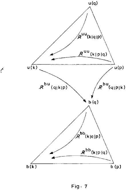
FIG. 1.:

FIG. 2.:

FIG. 3.:

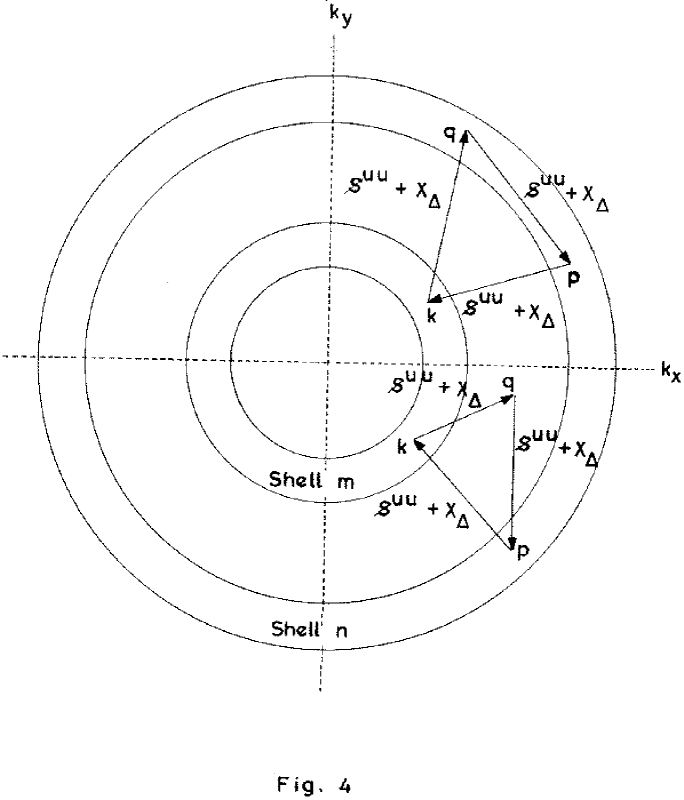
FIG. 4.:

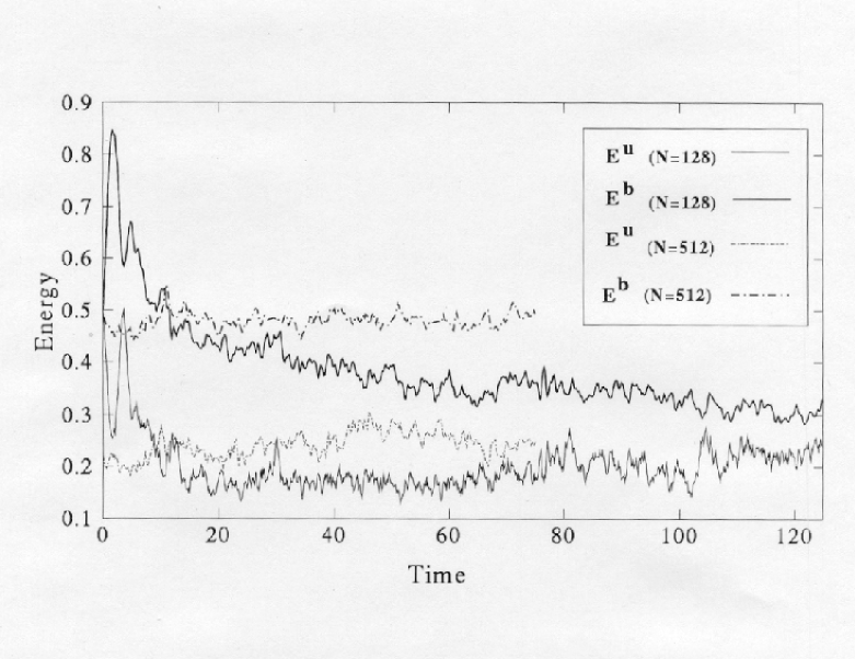
FIG. 5.:

FIG. 6.:

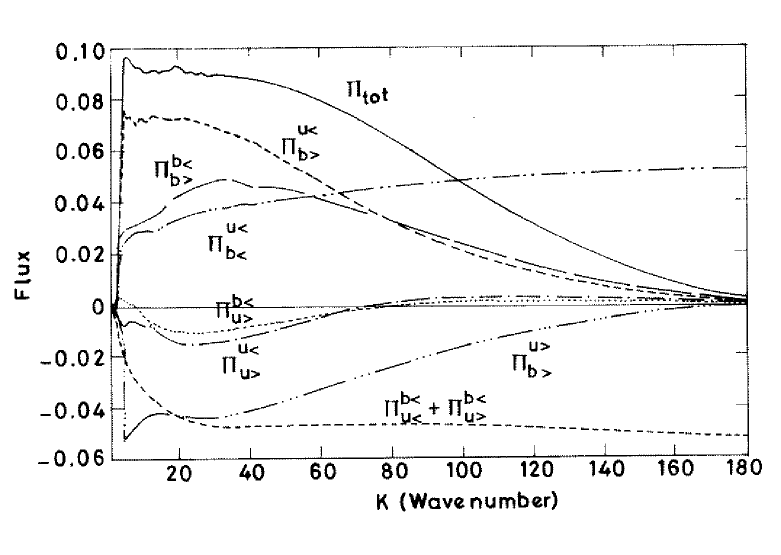
FIG. 7.:

FIG. 8.:

FIG. 9.:

FIG. 10.:

FIG. 11.:

FIG. 12.:

FIG. 13.:

FIG. 14.:

REFERENCES

- [1] M. K. Verma et al., J. Geophys. Res. 101, 21619 (1996).
- [2] W. C. Müller and D. Biskamp, Phys. Rev. Lett. 84, 475 (2000).
- [3] D. Biskamp and W. C. Müller, Phys. Plasma 7, 4889 (2000).
- [4] M. K. Verma, Phys. Plasma 6, 1455 (1999).
- [5] M. K. Verma, Phys. Rev. E 64, 26305 (2001).
- [6] M. K. Verma, Phys. Plasma 8, 3945 (2001).
- [7] S. Sridhar and P. Goldreich, Astrophys. J. 432, 612 (1994).
- [8] P. Goldreich and S. Sridhar, Astrophys. J. 438, 763 (1995).
- [9] A. Pouquet, U. Frisch, and J. Léorat, J. Fluid Mech. 77, 321 (1976).
- [10] A. Pouquet and G. S. Patterson, J. Fluid Mech. 85, 305 (1978).
- [11] G. K. Batchelor, Phys. Fluids B 1, 1964 (1989).
- [12] A. Pouquet, J. Fluid Mech. 88, 1 (1978).
- [13] A. Ishizawa and Y. Hattori, J. Phy. Soc. Jpn. 67, 4302 (1998).
- [14] A. Ishizawa and Y. Hattori, J. Phy. Soc. Jpn. 67, 441 (1998).
- [15] D. C. Montgomery, in Solar Wind Five, edited by M. Neugebauer (NASA Conf. Publ. CP-2280, Coplan MA, 1983), p. 107.
- [16] Y. B. Zeldovich, A. A. Ruzmaikin, and D. D. Sokoloff, Magnetic fields in Astrophysics (Gordon and Breach Science Publishers, New York, 1983).
- [17] P. Frick and D. Sokoloff, Phys. Rev. E 57, 4155 (1998).
- [18] M. M. Stanis̆ić, Mathematic Theory of Turbulence (Springer-Verlag, New York, 1988).
- [19] D. C. Leslie, Development in the Theory of Turbulence (Claredon, Oxford University Press, 1973).
- [20] G. Dar, Ph.D. thesis, I. I. T. Kanpur, 2000.
- [21] G. Dar, M. K. Verma, and V. Eswaran, physics/0006012 (2000).
- [22] J. A. Domaradzki and R. S. Rogallo, Phys. Fluids A 2, 413 (1990).
- [23] C. Canuto, M. Y. Hussaini, A. Quarteroni, and T. A. Zhang, Spectral Methods in Fluid Turbulence (Springer-Verlag, Berlin, 1988).
- [24] M. K. Verma, Phys. Plasmas (submitted), nlin.CD/0103033 (2001).
- [25] M. K. Verma, D. A. Roberts, and M. L. Goldstein, J. Geophys. Res. 100, 19839 (1995).