Breathing Current Domains in Globally Coupled Electrochemical Systems:
A Comparison with a Semiconductor Model

Abstract

Spatio-temporal bifurcations and complex dynamics in globally coupled intrinsically bistable electrochemical systems with an S-shaped current-voltage characteristic under galvanostatic control are studied theoretically on a one-dimensional domain. The results are compared with the dynamics and the bifurcation scenarios occurring in a closely related model which describes pattern formation in semiconductors. Under galvanostatic control both systems are unstable with respect to the formation of stationary large amplitude current domains. The current domains as well as the homogeneous steady state exhibit oscillatory instabilities for slow dynamics of the potential drop across the double layer, or across the semiconductor device, respectively. The interplay of the different instabilities leads to complex spatio-temporal behavior. We find breathing current domains and chaotic spatio-temporal dynamics in the electrochemical system. Comparing these findings with the results obtained earlier for the semiconductor system, we outline bifurcation scenarios leading to complex dynamics in globally coupled bistable systems with subcritical spatial bifurcations.

I Introduction

The focus of research in nonlinear dynamics has evolved from temporal instabilities over simple spatial patterns to complex spatio-temporal behavior and the control or synchronization of such dynamics. Complex spatio-temporal behavior in reaction-diffusion equations, which is in a wider sense the class of equations dealt with also in electrochemistry, might be found when instabilities breaking time and space symmetries interact. A generic case is the interaction of Turing Turing (1952) and Hopf bifurcation in a two component activator-inhibitor system in which the involved species diffuse. Complex spatio-temporal dynamics has been found near this codimension-two point theoretically Dewel et al. (1995); DeWit et al. (1996); Meixner et al. (1997) as well as experimentally Boissonade et al. (1995); Valette et al. (1994); Heidemann et al. (1993).

In electrochemical systems that can be described by a two component model one variable typically is of electrical nature and the associated transport mechanism is migration rather than diffusion Krischer (1999); Krischer et al. (2001). The decisive variable for the dynamics of the electric circuit is the double layer potential $\phi_{\rm DL}$, measuring the voltage drop across the interface between the working electrode and the electrolyte solution Koper (1996). Local perturbations in the double layer potential are mediated through the electric field in the electrolyte. Thus, spatial inhomogeneities in the double layer potential are felt not only by its nearest neighbors, but by a whole range of neighboring sites which makes the coupling nonlocal Mazouz et al. (1997a). The degree of non-locality depends on the geometry of the electrochemical cell, most importantly on the positions of the working (WE), counter (CE) and reference electrode (RE) with respect to each other Mazouz et al. (1997b). Furthermore it can be shown that the galvanostatic operation mode (constant current control) introduces an additional global coupling into the system Mazouz et al. (1998).

The role of the second variable in two component activator-inhibitor systems in electrochemistry is played, e. g., by the chemical concentration of the reacting species in the double layer or by the density of adsorbed molecules on the WE.

Over the last decade global coupling has been an active area of research. Global coupling is present in systems that are subject to external control, e.g. via an electric circuit (such as in electrochemical Flätgen and Krischer (1995); Grauel et al. (1998); Krischer et al. (2000); Mazouz et al. (1997b, 1998); Strasser et al. (2000); Christoph et al. (1999a, b); Kiss et al. (1999), semiconductor Volkov and Kogan (1969); Bass et al. (1970); Alekseev et al. (1998); Meixner et al. (2000, 1998); Bose et al. (2000); Schimansky-Geier et al. (1991); Schöll (2001) and gas discharge Willebrand et al. (1992) systems) or via the electric control of the temperature in catalytic reactors Barelko et al. (1977); Zhukov and Barelko (1982); Graham et al. (1993); Middya et al. (1993); Middya and Luss (1994); Annamalai et al. (1999). But global coupling may also be due to transport processes that happen on time scales much faster than all other relevant time scales in the system, e. g. fast mixing in the gas phase Mertens et al. (1993, 1994); Falcke and Engel (1994); Rose et al. (1996); Veser et al. (1993); Falcke and Engel (1997). A variety of other systems are described by dynamics that include global coupling, e.g., ferromagnetic Elmer (1990), biological Seung et al. (1995), and chemical systems in which the global coupling can be light induced Schebesch and Engel (1996); Vanag et al. (2000). Abstract theoretical models are discussed, e. g., in Battogtokh et al. (1997); Lima et al. (1998); Hempel et al. (1998).

Results regarding electrochemical systems with global coupling have been reported for systems with an N-shaped current-voltage characteristic (termed N-NDR systems: N-shaped negative differential resistance) for different types of global coupling. In these systems the double layer potential acts as an activator and global coupling introduced by the galvanostatic control mode was shown to accelerate front motion Flätgen and Krischer (1995); Mazouz et al. (1997a) thus having a synchronizing effect on the spatial dynamics. Desynchronizing global coupling of the activator was shown to stabilize potential fronts, leading to two stationary potential domains Grauel et al. (1998); Grauel and Krischer (2001). Also the formation of pulses and standing waves was observed Christoph et al. (1999a); Strasser et al. (2000); Otterstedt et al. (1996).

In electrochemical systems with an S-shaped current-voltage characteristic (S-NDR) the roles of activator and inhibitor are reversed, leading to a global coupling of the inhibitor under galvanostatic conditions. This leads to the opposite effects opposed to N-NDR systems, i.e. current domains that are stabilized by the constant current constraint Krischer et al. (2000). Similar results on accelerated and decelerated fronts in globally coupled semiconductors with S- or Z-shaped current-voltage characteristics have also been obtained Meixner et al. (2000).

In the present paper we focus on the latter case of global coupling of the inhibitor in an electrochemical system with an S-shaped current-voltage curve. Furthermore, we consider systems with high electrolyte conductivity. In such systems the migration coupling is so efficient that any spatial variation in $\phi_{\rm DL}$ can be neglected, which results in an additional global coupling Krischer et al. (2000). The set of equations to be investigated is thus of the general form:

$$\tau_{\phi_{\rm DL}}\frac{\partial\phi_{\rm DL}}{\partial t} = g(\phi_{\rm DL},\langle\theta\rangle_{G})$$ (1)

$$\tau_{\theta}\frac{\partial\theta}{\partial t} = f(\phi_{\rm DL},\theta)+D\Delta\theta,$$ (2)

where $\theta$ stands for the activator variable, whose dynamics comprises an autocatalytic chemical step. The angular brackets denote the spatial average over the spatial domain $G$. $f$ is autocatalytic in $\theta$; $g$ exhibits a monotonic characteristic as a function of $\phi_{\rm DL}$ and $\theta$. $\tau_{\phi_{\rm DL}(\theta)}$ denote the characteristic times for changes in $\phi_{\rm DL}$ and $\theta$, respectively.

A formally very similar set of equations describes the dynamics in bistable semiconductor systems operated via an external load resistance Volkov and Kogan (1969); Bass et al. (1970); Wacker and Schöll (1994a); Schöll (2001). The formation and dynamics of current density patterns in bistable semiconductors was extensively studied Bose et al. (1994); Wacker and Schöll (1994b); Wacker and Schöll (1995); Alekseev et al. (1998); Bose et al. (2000). In this respective class of semiconductor systems the current-voltage characteristic also resembles the shape of an S, which points to the fact that the roles of the dynamic variables are very similar to the electrochemical model: The voltage drop $u$ across a semiconductor device acts effectively as inhibitor, and it is subject to a global constraint imposed by the external electric circuit. The role of the activator variable might be played by different physical quantities, such as the electron temperature Volkov and Kogan (1969), the concentration of excess carriers Schöll (1987), the charge density in resonant tunneling structures Wacker and Schöll (1995); Glavin et al. (1997); Mel’nikov and Podlivaev (1998) (note that for bistable resonant tunneling structures the current-voltage characteristic is Z-shaped resulting in an activatory, not inhibitory effect of the global constraint), the voltage drop across pn-junctions in thyristors Gorbatyuk and Rodin (1992); Meixner et al. (1998) or the interface charge density in a heterostructure hot electron diode (HHED) Wacker and Schöll (1994b). The dynamic equations are of the same structural form as eq. (1),(2); only the local nonlinear functions $f$ and $g$ differ from the electrochemical model.

For the current density dynamics in a class of models originally derived for the HHED in one or two spatial dimensions under galvanostatic (current-controlled) conditions, interesting complex spatio-temporal patterns termed “spiking” and “breathing” current filaments were found Wacker and Schöll (1994a); Bose et al. (1994). Recently, a sufficient condition for the onset of such complex spatio-temporal dynamics was given Bose et al. (2000).

Realizing the obvious similarities, we show in this paper that the methods (e. g. for analyzing the dynamics) developed for the semiconductor system can be applied to gain insight into the interaction of different instabilities in the electrochemical system. Results regarding the possibility of the occurrence of complex spatio-temporal behavior and the mechanisms that lead to such behavior are given. It is emphasized whether the different dynamical regimes depend upon the general structural form of the equations, especially regarding the influence of global coupling, or if they are due to special properties of the underlying physical or chemical system, and thus the local dynamics. Hence a comparison of electrochemical and semiconductor systems gives considerable insight into generic complex dynamics of globally coupled bistable systems.

The paper is organized as follows. In the next section we introduce the electrochemical model, discuss its important parameters and the mechanisms leading to global coupling in the model. In the following section we characterize the dynamics of the model by linear stability analysis along the lines developed for the semiconductor model and by numerical simulations. In the discussion we compare the important features of the two models. The mechanism leading to complex spatio-temporal behavior in both models is different and this difference is explored in this section in some depth. We summarize our results in the last section and give a short outlook to applications in terms of experimental verifications and transfer of the electrochemical results to the semiconductor model.

II Model

The central variable in electrochemical pattern formation is the double layer potential $\phi_{\rm DL}$, the potential drop across the interface between the WE and electrolyte solution. The dynamic evolution equation for $\phi_{\rm DL}$ can be deduced from the local charge balance at the electrode/electrolyte interface.

To make things as transparent as possible and to facilitate later comparison with the semiconductor model, we employ the idealized geometry shown in fig. 1.

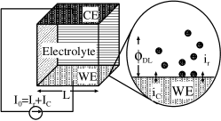
Figure 1: Schematic setup of the electrochemical system. A constant current $I_{0}$ is applied in a electrochemical cell consisting of a rectangular working electrode (WE), electrolyte, and a rectangular counter electrode (CE). WE and CE form top and bottom of the box-like cell with otherwise insulating walls. $\phi_{\rm DL}$ is the voltage drop across the interface. $i_{\rm r}$ and $i_{\rm C}$ symbolize reaction current density and capacitive current density, respectively.

WE and CE are equally sized rectangular plates positioned parallel to each other in a box-like cell with otherwise insulating walls. This geometry imposes no-flux boundary conditions for $\phi_{\rm DL}$ and $\theta$; there will be no spatial inhomogeneities of the electric field at the interface imposed by this geometry.

For very high electrolyte conductivities $\sigma$, spatial inhomogeneities in the double layer potential are damped out very fast via the efficient coupling through migration currents. It follows that spatial variations of $\phi_{\rm DL}$ can be neglected. This effectively introduces a global coupling in the system, since local perturbations in $\phi_{\rm DL}$ are felt instantaneously in the whole double layer.

In the following we additionally assume current controlled conditions. Galvanostatic control is known to introduce an additional global coupling into the system Mazouz et al. (1997b); Krischer et al. (2000). Assuming a specific double layer capacitance $C$, the dynamic equation for the double layer potential reads

$$C\frac{\partial\phi_{\rm DL}}{\partial t}=-i_{\rm r}(\phi_{\rm DL},\langle\theta\rangle)+i_{0},$$ (3)

where $i_{\rm r}(\phi_{\rm DL},\theta)$ is the reaction current density and $i_{0}$ denotes the imposed current density. The activator variable $\theta$ describes the evolution of the coverage of the WE by an adsorbate or the concentration of a chemical species in the reaction plane. Its dynamics will be modeled by an equation of the form (2), where we restrict our system to one spatial dimension (1d) since the qualitative behavior should also be captured on 1d domains. 1d domains also resemble the situation of a very large aspect ratio of the rectangular domain, where one spatial dimension is too small to allow for spatial instabilities and can thus be eliminated.

We use the following model functions for the local dynamics of the activator and the reaction current density $i_{\rm r}$

$$i_{\rm r}(\phi_{\rm DL},\theta) =(1-\theta)e^{\phi_{\rm DL}}$$ (4)

$$f(\phi_{\rm DL},\theta) =(1-\theta)e^{-\nu\phi_{\rm DL}^{2}-g\theta}-p\theta e^{\nu\phi_{\rm DL}^{2}+g\theta}$$ (5)

originally derived to describe pattern formation observed in a reaction, in which a reaction inhibiting adsorbate undergoes a first order phase transition due to lateral interactions of the adsorbate molecules Mazouz and Krischer (2000); Li et al. (2001). The transformations leading to dimensionless units differ from the ones given in Mazouz and Krischer (2000); the derivation is given in Appendix A. Note the non-polynomial nature of the function $f$.

The dimensionless set of equations is thus

$$\frac{\partial\phi_{\rm DL}}{\partial t} =\gamma(i_{0}-(1-\langle\theta\rangle)e^{\phi_{\rm DL}})$$ (6)

$$\frac{\partial\theta}{\partial t} =\mu\left((1-\theta)e^{-w(\theta,\phi_{\rm DL})}-p\theta e^{w(\theta,\phi_{\rm DL})}\right)+\frac{\partial^{2}\theta}{\partial x^{2}}$$ (7)

with

$$w(\theta,\phi_{\rm DL}) =\nu\phi_{\rm DL}^{2}+g\theta,$$

subject to the boundary conditions

$$\left.\frac{\partial\theta}{\partial x}\right|_{x=0,\pi}=0.$$

We normalize space to the interval $[0,\pi]$ for computational convenience and thus

$$\langle\theta\rangle=\frac{1}{\pi}\int_{0}^{\pi}\theta(x)\,{\rm d}x.$$

This leads to the proportionality of the parameters $\mu,\gamma\propto L^{2}$; $\mu$ and $\gamma$ still can be changed independently since also other physical quantities enter these parameters (cf. Appendix A).

In fig. (2a)

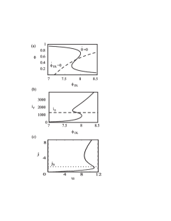
Figure 2: (a) Nullclines of the model (6),(7) for an imposed current density in the autocatalytic regime (solid line $\dot{\theta}=0$, dashed line $\dot{\phi_{\rm DL}}=0$, $i_{0}=1300$, for the other parameters see Appendix A). (b),(c) S-shaped current-voltage curve together with the load line $i_{0}$ ($j_{0}$) for the electrochemical (eq. (6),(7)) and the semiconductor (eq. (13),(14)) system, respectively.

the nullclines of the system are depicted for a current density $i_{0}$ that is set in the range of the negative differential resistance in the current-voltage characteristic (see fig. 2b). The S-shaped current-voltage-characteristic is depicted together with the load line $i=i_{0}$ in fig. 2b. This physically more intuitive ($i$-$\phi_{\rm DL}$)-plane representation will be used in the following.

The parameters $\nu$, $p$ and $g$ are fixed throughout this paper at the values $\nu=0.025$, $p=0.5$ and $g=-2.4$ (cf. Appendix A). The dynamics is determined by the model parameters $\mu$, essentially proportional to $L^{2}$, the relaxation time ratio of activator and inhibitor $\gamma/\mu$ (independent of $L$), and the general excitation level controlled by the imposed current density $i_{0}$. The relaxation time ratio can be accessed easily via the concentrations of the reacting and adsorbing species; $i_{0}$ is set by the galvanostatic control unit.

The numerical results discussed in section III.2 were obtained using pseudo spectral decomposition in space Canuto (1993) employing 15 spatial cosine-modes (the results do not change when a larger number of modes is chosen). For the integration in time the routine lsode Hindmarsh (1980) and for continuation of steady states and limit cycles the package AUTO Doedel and Kevernez (1986) was used.

III Stability Analysis and Simulations

III.1 Homogeneous Steady State

In this section we consider the spatially uniform fixed points of the system (6),(7) and their bifurcations. The uniform steady state $(\phi_{\rm DL}^{\rm ss},\theta^{\rm ss})$ is given by $i_{r}(\phi_{\rm DL}^{\rm ss},\theta^{\rm ss})=i_{0}$, $f(\phi_{\rm DL}^{\rm ss},\theta^{\rm ss})=0$ and corresponds to the homogeneous S-shaped current-voltage characteristic (fig. 2b). Perturbing the steady state with a perturbation $(\delta\phi_{\rm DL}e^{\lambda t},\delta\theta\cos(nx)e^{\lambda t})$ (consistent with the boundary conditions), the temporal evolution of the perturbation is given by the eigenvalues of the Jacobian matrix $J$

$$\lambda_{1,2}=\frac{{\rm tr}J}{2}\pm\sqrt{\frac{({\rm tr}J)^{2}}{4}-\det J}$$

and stability $({\rm Re}\lambda<0)$ implies that $(\det J>0\quad\wedge\quad{\rm tr}J<0)$. The Jacobian reads

$$J=\begin{pmatrix}-\gamma\sigma_{\rm r}&-\gamma i_{\rm r_{\theta}}\\ \mu f_{\phi_{\rm DL}}&\mu f_{\theta}-n^{2}\end{pmatrix}.$$

Subscripts denote partial derivatives with respect to the subscripted variable and evaluation at the steady state (e. g. $f_{\theta}=\left.\frac{\partial f}{\partial\theta}\right|_{(\phi_{\rm DL}^{\rm ss},\theta^{\rm ss})}$). For brevity we denote $\sigma_{\rm r}:=\left.\frac{\partial i_{\rm r}}{\partial\phi_{\rm DL}}\right|_{(\phi_{\rm DL}^{\rm ss},\theta^{\rm ss})}$.

The stability of the fixed point with respect to homogeneous fluctuations $(n=0)$ can be determined by inspecting

$$\det J = -\gamma\mu f_{\theta}(\sigma_{\rm r}-\frac{f_{\phi_{\rm DL}}}{f_{\theta}}i_{\rm r_{\theta}})$$

$$= -\gamma\mu f_{\theta}\left(\sigma_{\rm r}+i_{\rm r_{\theta}}\frac{{\rm d}\theta^{\rm ss}(\phi_{\rm DL})}{{\rm d}\phi_{\rm DL}}\right)$$

$$= -\gamma\mu f_{\theta}\frac{{\rm d}i_{r}(\theta^{\rm ss}(\phi_{\rm DL}),\phi_{\rm DL})}{{\rm d}\phi_{\rm DL}}$$

and

$${\rm tr}J=\mu f_{\theta}-\gamma\sigma_{\rm r}.$$

Obviously $\det J>0$ in general since $\mu,\gamma>0$ and $f_{\theta}\frac{{\rm d}i_{r}(\theta^{\rm ss}(\phi_{\rm DL}),\phi_{\rm DL})}{{\rm d}\phi_{\rm DL}}<0$, which follows from the fact that the branch of negative differential resistance ($\frac{{\rm d}i_{r}(\theta^{\rm ss}(\phi_{\rm DL}),\phi_{\rm DL})}{{\rm d}\phi_{\rm DL}}<0$) is caused solely by the activator variable $\theta$, equivalent to saying that $\sigma_{\rm r}>0$ in general.

However, tr $J$ might change sign on the NDR-branch since $f_{\theta}>0$ and $\sigma_{\rm r}>0$, which leads to an oscillatory instability (Hopf bifurcation) of the homogeneous steady state (denoted by a superscript “h”, cf. table 1) at

Table 1: Abbreviations for bifurcation points

h	Hopf bifurcation of the homogeneous steady state
d	domain bifurcation of the homogeneous steady state
sn-d	saddle-node bifurcation of domains
hd	Hopf bifurcation of the domain state
snp	saddle-node bifurcation of breathing domains, i. e.  periodic orbits
DH	domain-Hopf codimension-two point (d and h)
TB	Takens-Bogdanov codimension-two point (sn-d and hd)
DHD	degenerate Hopf bifurcation of domains (snp and hd)

$$\left(\frac{\gamma}{\mu}\right)^{\rm h}=\frac{f_{\theta}}{\sigma_{\rm r}}.$$ (8)

Thus for $\gamma/\mu<\left(\gamma/\mu\right)^{\rm h}$ (low concentration of the reacting species or high concentration of the adsorbate) the homogeneous steady state is unstable in a certain $i_{0}$-interval, since $f_{\theta}\sigma_{\rm r}^{-1}$ depends on the imposed current density via the steady state condition. When plotting the critical value $\left(\gamma/\mu\right)^{\rm h}$ as a function of the imposed current density fig. 3a is obtained.

Figure 3: (a) Location of the Hopf-bifurcation of the homogeneous steady state in the ($\gamma/\mu$-$i_{0}$)-parameter-plane for the electrochemical model (6),(7). For $\gamma/\mu>2.2\cdot 10^{-4}$ the system is stable with respect to homogeneous fluctuations. (b) Threshold for the spatial instability of the uniform steady state in the ($\mu$-$i_{0}$)-plane. For system sizes smaller than $\mu_{\rm min}=3.54$ the system is stable with respect to spatial fluctuations. (c) Critical system size $L_{\rm cr}$, of the spatial instability for the semiconductor model (eq. (13),(14)) as a function of the imposed current density $j_{0}$.

For $\gamma/\mu>(\gamma/\mu)^{\rm h}_{\rm max}=2.2\cdot 10^{-4}$ there are no oscillatory solutions for any $i_{0}$ and for $\gamma/\mu\ll(\gamma/\mu)^{\rm h}_{\rm max}$ the oscillatory instability takes place close to the turning points of the current-voltage characteristic at $i_{0}=889$ and $i_{0}=1587$.

To determine the stability with respect to spatially inhomogeneous fluctuations, it is sufficient to consider the activator variable $\theta$, since sinusoidal perturbations do not affect the average value of $\theta$ and thus the double layer dynamics. Therefore the steady state becomes unstable with respect to the $n^{\rm th}$-mode for

$$\mu>\frac{n^{2}}{f_{\theta}},$$

and the first mode to become unstable is always the mode with wavenumber one Mikhailov (1990). The wavelength of the first unstable mode depends on the system size and is equal to $2L$ for Neumann boundary conditions. In the following we term this instability domain bifurcation. The critical parameter value is thus:

$$\mu^{\rm d}=f_{\theta}^{-1}.$$ (9)

This critical value is depicted in fig. 3b as a function of $i_{0}$. For systems sizes $\mu<\mu_{\rm min}=3.54$ the spatial instability is suppressed; this defines a natural length scale for the system. For system sizes much larger than this natural length scale the spatial instabilities occur once again close to the turning points of the current-voltage characteristic.

The spatial and oscillatory instabilities may coincide in a codimension-two point (Domain-Hopf bifurcation, “DH”, cf. table 1) if

$$\gamma^{\rm DH}=\sigma_{\rm r}^{-1}.$$ (10)

The respective imposed current density value $i_{0}^{\rm DH}(\mu)$ is defined as the solution of (9) with respect to $i_{0}$.

III.2 Homogeneous Limit Cycle and Stationary Domains

In this section we complete the picture of the different basic attractors of the model by including limit cycles and stationary current domains into our stability analysis. Analytical methods fail in most cases since the involved bifurcations are either subcritical and thus do not allow for an amplitude equation analysis and/or the considered system sizes are intermediate, which excludes methods like singular perturbation theory Kerner and Osipov (1994) to describe domain interface dynamics.

For common concentrations and system sizes the double layer dynamics will be much faster than the dynamics of the activator. For these conditions the parameters $\gamma$ and $\mu$ will be of the order 10 and 100, respectively. It follows that in most cases oscillatory instabilities are not present in the system and the only nontrivial mode is a stationary current domain as depicted in fig. 4a

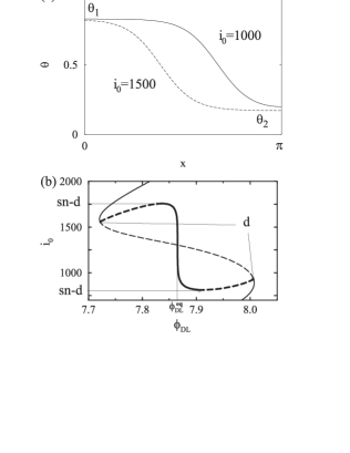
Figure 4: (a) Stable domains for two values of the imposed current density $i_{0}$ for the electrochemical model ($\mu=25$, $\gamma=10$). (b) Bifurcation diagram for $\mu=25$ and $\gamma=10$. Shown is $\phi_{\rm DL}$ as a function of the bifurcation parameter $i_{0}$ in the familiar current-potential plane. The branch of negative differential resistance is unstable (thin dashed line) with respect to domain formation. The domain branches (thick lines) bifurcate subcritically (d) near the turning points of the current-voltage characteristic. The stable and unstable domain branches (solid resp. dashed thick lines) are born in a saddle-node bifurcation of domains (sn-d). The domain branch can be approximated by an equal-areas rule, eq. (11), in a huge $i_{0}$ interval yielding an equistability potential $\phi_{\rm DL}^{\rm eq}$.

for two values of $i_{0}$. This current domain is the final state of the system in the spatially unstable regime and the mechanism leading to such a stationary domain is well known (e. g. Mikhailov (1990); Krischer et al. (2000)):

The activator is bistable as a function of the double layer potential. An overcritical local fluctuation in a system without global coupling that is prepared in the metastable state would lead to the formation of a transition front to the globally stable state. The global constraint, however, forces the system to maintain an average current. The system meets this constraint by taking on an inhomogeneous state in which two phases coexist. With other words, the front velocity becomes zero. The final state of the system is described by a Maxwell type construction: the intermediate, equistability double layer potential $\phi_{\rm DL}^{\rm eq}$, which is established in the stationary structure is determined by the equal-areas rule Mikhailov (1990); Schöll (2001)

$$\int_{\theta_{1}}^{\theta_{2}}f(\phi_{\rm DL}^{\rm eq},\theta)\,{\rm d}\theta=0.$$ (11)

In fig. 4b the bifurcation diagram with respect to $i_{0}$ is shown for $\mu=25$, $\gamma=10$. Even though the system size is comparable to the interface width, as can be seen in fig. 4a, the above construction holds for a wide $i_{0}$-interval. However, since the arguments given above apply strictly only for infinite systems, deviations near the turning points of the current-voltage characteristic of the domain are clearly visible. These deviations represent a boundary effect.

States with several domains are unstable due to the winner takes all principle Volkov and Kogan (1969); Schimansky-Geier et al. (1991). Domains with an extremum not located at the boundaries are unstable with respect to translation and will be attracted by the boundary.

Fig. 4b also shows that spatially patterned solutions typically bifurcate subcritically from the homogeneous state and meet the stable domain-branch in a saddle-node bifurcation (sn-d, cf. table 1). The domains remain stable in the whole $i_{0}$-interval in which the current-voltage characteristic of the domain exhibits a negative differential resistance for these parameter values. This behavior can also be rationalized analytically Bass et al. (1970); Alekseev et al. (1998). The domain bifurcation is supercritical only in a small $\mu$-interval close to the minimal system size $\mu_{\rm min}$.

When $\mu$ is fixed at a value $\mu>\mu_{\rm min}$ and the double layer dynamics is slowed down to $\gamma$ below $\mu(\gamma/\mu)^{\rm h}_{\rm max}$, the additional mode of homogeneous oscillations becomes present in the system. For $\gamma\lesssim\mu(\gamma/\mu)^{\rm h}_{\rm max}$ it bifurcates supercritically from the spatially unstable state, therefore small amplitude oscillations will be unstable with respect to spatial fluctuations for any $i_{0}$. With increasing oscillation amplitude (decreasing $\gamma$) the oscillations become stabilized in a pitchfork bifurcation (cf. fig. 5a).

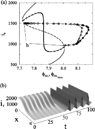
Figure 5: (a) Bifurcation diagram for the electrochemical model ($\mu=25$, $\gamma=3\cdot 10^{-3}$). Apart from the branches shown in fig. 4b, a branch of unstable homogeneous oscillatory solutions (open circles) bifurcates supercritically (h) near the turning points of the current-voltage characteristic. Shown is the maximum value of $\phi_{\rm DL}$ during one oscillation cycle. After stabilization through a pitchfork bifurcation, the stable homogeneous oscillations (full circles) are separated from the stable domains by an unstable inhomogeneous limit cycle (open triangles). (b) Typical scenario of an oscillatory instability of a domain for lower values of $\gamma$ than in (a) ($\mu=25$, $\gamma=1\cdot 10^{-4}$, $i_{0}=1000$). Shown is the reaction current density $i_{r}=(1-\theta)e^{\phi_{\rm DL}}$ as a function of space and time. At these parameter values the oscillatory instability of the domain is subcritical and the system finally settles down to homogeneous relaxation oscillations (standard scenario).

This results in bistability of stationary domains and an uniform limit cycle in an intermediate $i_{0}$-interval. The basins of attraction are separated by an unstable inhomogeneous limit cycle.

If $\gamma$ is lowered even further, the stationary current domain will become unstable also. This can be rationalized by recalling that the stabilization mechanism of the domains is the positive global coupling on $\phi_{\rm DL}$. If the delay of the double layer dynamics becomes too large, $\phi_{\rm DL}$ can no longer control the interface stability. We denote the critical value of this oscillatory instability of the domain by $\gamma^{\rm hd}(\mu,i_{0})$ (cf. table 1). Numerical simulations show that the threshold for an oscillatory instability of the current domain lies typically below the threshold for the Hopf bifurcation of the homogeneous steady state

$$\gamma^{\rm hd}(\mu,i_{0})<\gamma^{\rm h}(\mu,i_{0}).$$ (12)

This can be understood in the frame of the eigenmodes of the current domain for large system sizes if we recall that in absence of global coupling the domain state has only one positive eigenvalue that tends to zero with increasing system size. The respective arguments are given in Alekseev et al. (1998). The numerical investigations show that relation (12) in general holds for small and intermediate system sizes also.

It follows that, in general, the homogeneous relaxation oscillations represent an attractor when the domain loses stability. The oscillatory instability of the domain is usually subcritical; a state close to the domain is eventually attracted by the stable homogeneous limit cycle (see fig. 5b). This can be regarded as the standard scenario (i. e. it exists in a wide parameter range) of a domain instability in globally coupled electrochemical systems with an S-shaped current-voltage characteristic. In this case no complex spatio-temporal behavior arises in the model.

III.3 Breathing Current Domains

We would expect complex spatio-temporal behavior if the branch of inhomogeneous limit cycle solutions that bifurcates from the domain-branch at the point of the oscillatory instability of the domain becomes stabilized or bifurcates supercritically. In this case the system would exhibit bistability between a stable inhomogeneous limit cycle and a stable homogeneous one. We did indeed find such a situation in the model for comparatively small system sizes ($\mu\sim 10$) and relaxation times well below the onset of homogeneous oscillations ($\gamma/\mu\sim 7\cdot 10^{-5}$). The instability leading to such complex spatio-temporal behavior is shown in fig. 6.

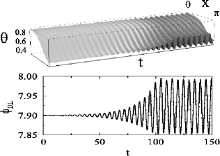
Figure 6: Oscillatory instability of a domain leading to stable, periodically breathing current domains for the electrochemical model ($\mu=10$, $\gamma=7\cdot 10^{-4}$, $i_{0}=1000$). (In this simulation a stable domain was prepared, $\gamma$ was lowered to $\gamma=7\cdot 10^{-4}$, and a small random fluctuation was added.)

In fig. 7a

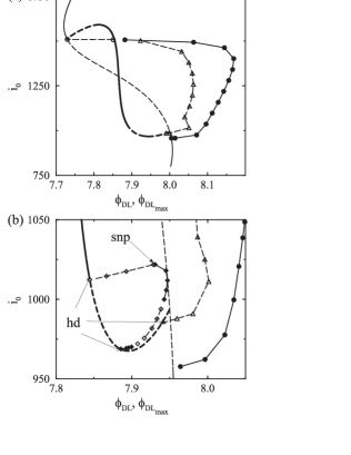
Figure 7: (a) Basis bifurcation diagram for stable periodic breathing for the electrochemical model ($\mu=10$, $\gamma=7\cdot 10^{-4}$). The oscillatory branch of the homogeneous limit cycles bifurcates supercritically before the spatial instability and thus homogeneous oscillations are stable nearly in the whole $i_{0}$-interval (full circles). The equal areas rule, eq. (11), fails for this system size. The domain branch (thick line) is unstable in a region of negative differential resistance (dashed thick line) near the lower saddle node bifurcation of domains. Marked with open triangles is an unstable inhomogeneous limit cycle. It is born in a pitchfork bifurcation of the homogeneous limit cycle at high $i_{0}$ and terminates in the unstable domain branch. (b) Enlargement of the bifurcation diagram at the lower turning point. Here also the branches of the inhomogeneous breathing mode are shown (diamonds). The breathing mode bifurcates subcritically (hd) from the domain branch at higher $i_{0}$ (open diamonds) and stable breathing (full diamonds) originates in an snp. In the projection of the limit cycle on the double layer potential it gets close to the homogeneous steady state but not in real phase space (cf. text). In the current density interval between approx. $i_{0}=1000$ and $i_{0}=975$ the inhomogeneous limit cycle undergoes a period doubling cascade leading to chaotic breathing (open diamonds).

the corresponding bifurcation diagram for $\mu=10$ and $\gamma=7\cdot 10^{-4}$ is depicted.

Decreasing the imposed current density from values in the regime of bistability between a stable domain and homogeneous oscillations, the domain branch exhibits an oscillatory instability (hd). The branch of solutions that bifurcates subcritically is stabilized via a saddle-node bifurcation of oscillatory domains, i. e.  periodic orbits (snp, cf. table 1), which can be seen in the enlarged bifurcation diagram, fig. 7b. The spatio-temporal behavior becomes more involved as the imposed current density $i_{0}$ is decreased. The limit cycle undergoes a period doubling cascade leading to stable chaotic spatio-temporal motion (fig. 8).

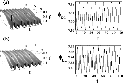
Figure 8: (a) Periodically breathing domains with period two at $i_{0}=990$ and (b) chaotically breathing domains at $i_{0}=980$ ($\mu=10$, $\gamma=7\cdot 10^{-4}$).

Decreasing $i_{0}$ further, a reversed period doubling cascade occurs which leads again to stable period one breathing domains. This branch then ends in a supercritical Hopf bifurcation of the domain very close to the saddle-node bifurcation, in which stable and unstable domains originate (sn-d). It is interesting to note that the dynamic nature of the invariant set that separates the basins of attraction of the two limit cycles is changing with increasing imposed current density from the unstable stationary domain (saddle point) to an unstable inhomogeneous limit cycle (see fig. 7b for low $i_{0}$).

The region in the ($i_{0}$-$\gamma$)-parameter-plane in which such complex spatio-temporal dynamics is found is depicted in fig. 9 for $\mu=10$.

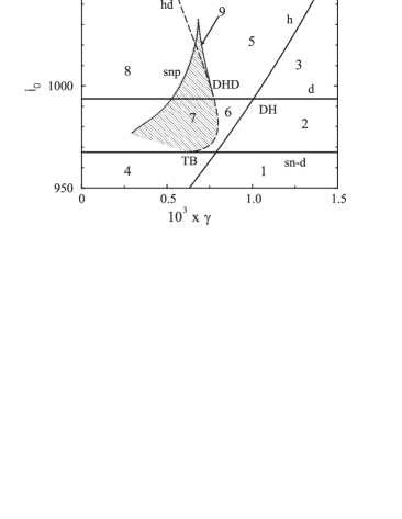
Figure 9: Existence region of stable periodic breathing in the ($i_{0}$-$\gamma$)-control-parameter plane (hatched region) for the electrochemical model ($\mu=10$). The main dynamic regimes, characterized by attractors, are indicated by the numbers 1–9; the attractors are given in table 2. Shown in solid lines are the lines of the domain bifurcation (d) and the saddle-node bifurcation in which the domains originate (sn-d) (both independent of $\gamma$). The domain bifurcation and the Hopf bifurcation of the homogenous steady state (h, solid) intersect in a Turing-Hopf-type codimension-two point (DH). The dashed line shows the oscillatory instability of the domain (hd). Denoted by snp (solid line) is the line of the saddle node bifurcation of periodic orbits, i. e. breathing domains.

Table 2: Dynamic regimes indicated in fig. 9

(1)	One stable homogeneous fixed point.
(2)	Bistability between stable domain and homogeneous fixed point.
(3)	Only one stable domain.
(4)	One stable homogeneous limit cycle.
(5)	Stable or unstable homogeneous limit cycle (cf. Appendix B) and stable domain.
(6)	Stable homogeneous limit cycle and stable domain.
(7)	Stable breathing current domains (periodic or chaotic) and a stable homogeneous limit cycle.
(8)	The Hopf bifurcation of the domain is subcritical, thus only stable homogeneous oscillations are present.
(9)	Region in which three attractors exist (cf. fig. 7 for $i_{0}\cong 1010$): Stable domains, stable breathing domains, and stable homogeneous limit cycle.

The lines of the Hopf bifurcation and the domain bifurcation of the homogeneous steady state and their intersection point (DH) are shown. The main regions that were discussed above (and in part also exist for different values of $\mu$) are indicated. Note the existence of three codimension-two points: The point in which domain and Hopf bifurcation coincide (DH) was discussed in sec. III.1. At the DH the system has a pair of purely imaginary eigenvalues and a real eigenvalue equal to zero Guckenheimer and Holmes (1983). Unfoldings of the DH have a further fine structure as discussed in Appendix B; it is not shown in fig. 9 for clarity. Denoted by TB is the point where saddle-node and Hopf-bifurcation meet (Takens-Bogdanov point) Guckenheimer and Holmes (1983). Note that in our case both bifurcations involve inhomogeneous steady states (i. e. domains) rather than homogeneous solutions. Left of the TB two saddle fixed points with one and three unstable directions, respectively, originate from the saddle-node bifurcation, right of it a saddle fixed point and a stable node. Again the fine structure, most remarkably a homoclinic bifurcation that should be present in the vicinity of the TB, is omitted. The third codimension-two point is a degenerate Hopf bifurcation of domains (DHD), in which the saddle-node bifurcation of periodic orbits (snp) coincides with the Hopf-bifurcation of the domain (hd).

We omitted in the bifurcation diagram (fig. 9) some of the branches mentioned above. Furthermore there are indications of the presence of additional bifurcations that determine the exact location of the lower boundary of the regime of complex behavior. Its detailed study is beyond the scope of this paper.

IV Comparison and Discussion

In this section we compare the different dynamic instabilities and regimes described in the previous section with results obtained earlier for the semiconductor model. The semiconductor model used has the (nondimensionalized) form

$$\dot{a} =\frac{u-a}{(u-a)^{2}+1}-0.05a+\frac{\partial^{2}a}{\partial x^{2}}$$ (13)

$$\dot{u} =\alpha(j_{0}-u+\langle a\rangle_{L}),$$ (14)

where $u$ denotes the potential drop across the semiconductor device (corresponding to $\phi_{\rm DL}$) and $a$ describes the interface charge density in the HHED (corresponding to $\theta$). The system length is $L$ and thus $\langle a\rangle_{L}=L^{-1}\int_{0}^{L}a\,{\rm d}x$. The current-voltage characteristic of the HHED is given by $j=u-a$. It also has the shape of an ‘S’ (fig. 2c). If space is rescaled to the interval $[0,\pi]$, the model exhibits the same structural dependence on three parameters as eqs. (6),(7)

$$\dot{a} =\mu^{\rm(s)}\left(\frac{u-a}{(u-a)^{2}+1}-0.05a\right)+\frac{\partial^{2}a}{\partial x^{2}}$$ (15)

$$\dot{u} =\gamma^{\rm(s)}(j_{0}-u+\langle a\rangle_{\pi}),$$ (16)

with $\mu^{\rm(s)}=\left(\frac{L}{\pi}\right)^{2}$ and $\gamma^{\rm(s)}=\left(\frac{L}{\pi}\right)^{2}\alpha$. These parameters can be interpreted in the same way as in the electrochemical model.

The two models possess equivalent basic modes: The branch of negative differential conductivity is unstable with respect to spatial perturbations for sufficiently large system sizes $L>L_{\rm min}$ (cf. fig. 3c) and to homogeneous oscillations for sufficiently slow dynamics of the voltage drop $u$ (small $\alpha$). However the temporal instability of the filament may lead to qualitatively different spatio-temporal dynamics. Apart from the breathing mode that the semiconductor models also exhibit, Schöll and Drasdo (1990); Wacker and Schöll (1994b); Bose et al. (2000); Schöll (2001) the system displays a complex spatio-temporal mode termed spiking (see fig. 10a) Wacker and Schöll (1994a); Bose et al. (1994).

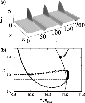
Figure 10: (a) Spiking current filament in 1d ($L=40$, $\alpha=0.035$, $j_{0}=1.2$). (b) Bifurcation diagram for the semiconductor system for complex spatio-temporal dynamics ($L=40$, $\alpha=0.06$). Shown is the potential drop across the semiconductor $u$ resp. the maximum $u$ during one oscillation versus the imposed current density $j_{0}$ at the lower turning point of the current-voltage characteristic. In the current-interval shown by the dashed lines no trivial state of the system is stable. The lower boundary is the spatial instability of the homogeneous steady state (thin lines) and the upper one is the oscillatory instability of the filament (thick lines). Homogeneous oscillations are not present in this current density interval, they bifurcate at higher current density values (open circles in the upper right corner). The resulting inhomogeneous oscillations (diamonds) that bifurcate subcritically from the stable domain branch are born by a saddle-node bifurcation of periodic orbits.

This mode evolves because the spatially inhomogeneous limit cycle that constitutes breathing comes eventually, with decreasing $\gamma$, very close to the homogeneous fixed point. This points to a structurally different dynamic regime as compared to the electrochemical system and facilitates the formulation of a sufficient condition for the occurrence of complex spatio-temporal dynamics Bose et al. (2000). In the following this will be explained in some detail.

Consider the bifurcation diagram of the semiconductor model for parameter values at which complex spatio-temporal dynamics is found (fig. 10b). Let us denote by $j_{0}^{\rm d}(\mu)$, $j_{0}^{\rm h}(\mu,\gamma)$ and $j_{0}^{\rm hd}(\mu,\gamma)$ the parameter values at which the spatial instability of the homogeneous steady state, the oscillatory instability of the homogeneous steady state and the oscillatory instability of the filament, respectively, occur. For an interval of imposed current densities $j_{0}$ no trivial state is stable, since, in contrast to the electrochemical model, homogeneous oscillations are not present in the system for imposed current density values within this interval, however the filament is already oscillatorily unstable ($\gamma^{\rm hd}(\mu,i_{0})>\gamma^{\rm h}(\mu,i_{0})$). Thus a sufficient condition for complex dynamics is

$$j_{0}^{\rm h}(\mu,\gamma)>j_{0}^{\rm d}(\mu)\quad\wedge\quad j_{0}^{\rm hd}(\mu,\gamma)>j_{0}^{\rm d}(\mu).$$

The limit case $j_{0}^{\rm hd}(\mu,\gamma)=j_{0}^{\rm h}(\mu,\gamma)=j_{0}^{\rm d}(\mu)\equiv j_{0}^{\rm DH}(\mu)$ can be reformulated as a condition for the timescale of the inhibitor $\gamma$ such that the condition can be tested for different system sizes Bose et al. (2000):

$$\gamma^{\rm hd}(i_{0}^{\rm d}(\mu))>\gamma^{\rm DH}(\mu).$$ (17)

The above inequality becomes clear, if one considers that the oscillatory instability of the filament is shifted toward higher imposed current density values when lowering $\gamma$, whereas the Hopf bifurcation point of the homogeneous steady state behaves in the opposite way and the spatial instability does not depend on $\gamma$.

In fig. 11

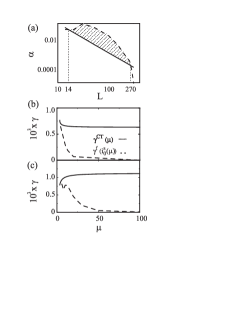
Figure 11: Thresholds for oscillatory instabilities at imposed current density values at which the homogeneous steady state becomes unstable with respect to spatial fluctuations (effective three parameter continuation) to test condition (17). The threshold for an oscillatory instability of the domain ($\gamma^{\rm hd}(i_{0}^{\rm s}(\mu))$) and the codimension-two point (DH) analogous to a Turing-Hopf codimension-two bifurcation ($\gamma^{\rm DH}(\mu)$) are shown as dashed and solid lines, respectively. In (a) the two curves are shown for the semiconductor system (double logarithmic plot) for 2d domains at the lower turning point of the current-voltage characteristic. The hatched region indicates the region in which the sufficient condition (17) for complex spatio-temporal dynamics is fulfilled. In (b) and (c) $\gamma^{\rm hd}(i_{0}^{\rm s}(\mu))$ and $\gamma^{\rm DH}(\mu)$ are shown for the electrochemical model for the two domain bifurcations at low and high current densities, respectively.

both critical timescales are plotted for both models. For the electrochemical model the critical timescales are also shown for the upper part of the S-shaped current-voltage characteristic. The above arguments do equally apply for this region. As indicated by the hatched region for the semiconductor system in fig. 11a, condition (17) is fulfilled for a large interval of system sizes $L$ (resp. $\mu^{\rm(s)}$) for the lower part of the S-shaped current-voltage characteristic. Apart from spiking, a broad variety of periodic and chaotic spatio-temporal modes has been found in this interval Bose et al. (2000). Condition (17) is never found to hold for the upper part for the semiconductor model (not shown). It can be seen in fig. 11b and 11c for the upper and lower part of the S-shaped current-voltage characteristic, respectively, that condition (17) is apparently never fulfilled in the electrochemical system for any system size.

Thus also the absence of spiking in the electrochemical system is easily understood; spiking evolves when the breathing mode eventually comes very close to the plane of homogeneous modes which constitutes a stable focus in this plane. The relaxation close to the homogeneous fixed point in the plane of the homogeneous modes leads to the small, almost homogeneous, oscillations and then the spike evolves again as the trajectory leaves the plane of homogeneous dynamics along the unstable direction of the homogeneous fixed point (cf. fig. 10). In the electrochemical system the plane of homogeneous modes always constitutes an unstable focus for parameter values in which the domain loses stability and thus the trajectory of inhomogeneous oscillations never comes close to the unstable homogeneous fixed point.

V Conclusions

The comparison of the two models presented in this paper allows us to identify bifurcations that exist in bistable systems subject to global inhibition. Apart from electrochemical and semiconductor systems such dynamics might be encountered in a variety of other systems, e. g. gas discharge devices Raizer (1997).

Stationary large amplitude spatial patterns called domains or filaments appear via a subcritical spatial bifurcation of the uniform state and form attractors in the whole range of effective autocatalysis for common parameter values in such systems. A characteristic length scale can be defined that facilitates quantitative comparison of the respective models. For comparable timescales of activator and inhibitor stable homogeneous relaxation oscillations can be expected. For slow dynamics of the globally coupled inhibitor oscillatory instabilities of the domains occur, initially near the turning points of the current-voltage characteristic of the domain. However, the routes to complex spatio-temporal patterns depend on the local dynamics and might thus differ in each individual system under consideration.

We have identified the following scenarios: If the Hopf bifurcation of the domain is supercritical, the system will display stable breathing domains. In the case of a subcritical bifurcation the dynamics depends upon the further structure of the bifurcation diagram. If condition (17) is fulfilled, the onset of stable breathing or spiking modes can be expected. When inequality (17) is not fulfilled and the oscillatory instability of the domain is subcritical, no general statement regarding the resulting dynamics is possible. Either homogeneous relaxation oscillations or complex spatio-temporal dynamics may result in this case.

We have demonstrated the above general statements with two models exhibiting different scenarios leading to stable complex spatio-temporal dynamics, thus illustrating the general scheme. Condition (17), which ensures that stationary or uniform modes are either unstable or do not exist, is fulfilled for the semiconductor system in a wide parameter range, but it can never be satisfied in the specific electrochemical model (6),(7). As a consequence the electrochemical breathing current domains always coexist with homogeneous oscillations. Thus they have a small basin of attraction compared to the situation in the semiconductor model (13),(14) where no other mode is stable in a certain parameter range. As another consequence spiking current filaments are only present in the semiconductor system. Complex dynamics could only be found near the turning point of the current-voltage characteristic corresponding to the lower value of the imposed current density in both systems.

These results emphasize the necessity to incorporate the spatial degree of freedom when studying electrochemical systems with negative differential resistance. Breathing current domains constitute a qualitatively new mode of complex spatio-temporal dynamics in electrochemical systems reported here for the first time. This mode may evolve to chaotic spatio-temporal dynamics via a period doubling cascade.

It should be noted that recent experimental studies of the CO-oxidation on Pt-single crystal electrodes have shown small amplitude oscillations of the potential in the range of negative differential resistance Koper et al. (2001). This system might be an experimental illustration of the above results, and therefore spatially resolved measurements would be desirable.

Appendix A Non-dimensionalization

In this section we give the transformations yielding the dimensionless model equations (4),(5). In physical units the equations read Mazouz and Krischer (2000)

$${\rm C}_{0}\frac{{\rm d}\phi_{\rm DL}}{{\rm d}t} ={\rm i_{0}^{\prime}}-{\rm\chi nF\bar{c}_{\rm r}k_{\rm r}}(1-<\theta>)$$

$$\quad\cdot\exp\left(\chi\frac{\rm\alpha nF}{RT}(\phi_{\rm DL}-\widetilde{\rm V})\right)$$

$$\frac{\partial\theta}{\partial t} ={\rm k_{\rm ad}\bar{c}_{\rm ad}}(1-\theta)\exp\left(-\alpha w^{\prime}(\phi_{\rm DL},\theta)\right)$$

$$\quad-{\rm k_{\rm d}}\theta\exp\left((1-\alpha)w^{\prime}(\phi_{\rm DL},\theta)\right)$$

with

$$w^{\prime}(\phi_{\rm DL},\theta) =\frac{\rm C_{0}-C_{1}}{\rm 2N_{\rm max}k_{\rm B}T}\phi_{\rm DL}^{2}+\frac{{\rm g^{\prime}}\theta}{\rm RT}.$$

The meaning of the numerous constants is given in Mazouz and Krischer (2000) and typical values of the constants are shown in table 3.

Table 3: Typical parameter values

${\rm k_{\rm ad}}$=	$1\cdot 10^{4}\frac{\rm cm^{3}}{\rm mol\ s}$		${\rm C_{0}}$=	$20\cdot 10^{-6}\frac{\rm C}{\rm V\ cm^{2}}$
${\rm k_{\rm d}}$=	$5\cdot 10^{-3}\rm s^{-1}$		${\rm C_{1}}$=	$2\cdot 10^{-6}\frac{\rm C}{\rm V\ cm^{2}}$
${\rm k_{\rm r}}\exp(-\frac{\rm\alpha nF}{\rm RT}\widetilde{\rm V})$=	$2\cdot 10^{-8}\frac{\rm cm}{\rm s}$		$\bar{\rm c}_{\rm ad}$=	$1\cdot 10^{-6}\frac{\rm mol}{\rm cm^{3}}$
${\rm N_{\rm max}}$=	$1\cdot 10^{14}{\rm cm^{-2}}$		${\rm D_{\theta}}$=	$1\cdot 10^{-5}\frac{\rm cm^{2}}{\rm s}$
${\rm n}$=	$1$		${\rm g^{\prime}}$=	$-1.2\cdot 10^{5}\frac{\rm J}{\rm mol}$
$\chi$=	$1$		$\alpha$=	$1/2$
${\rm T}$=	$300{\rm K}$

The model equations (4),(5) are retained via the transformations of the variables according to

$$\phi_{\rm DL}\rightarrow\phi_{\rm DL}^{\prime} =\frac{\rm\alpha nF}{\rm RT}\phi_{\rm DL}$$

$$t\rightarrow t^{\prime} =\frac{\rm\pi^{2}D_{\rm\theta}}{\rm L^{2}}t$$

$$x\rightarrow x^{\prime} =\frac{\pi}{\rm L}x,$$

and with the introduction of the parameters

$$\mu = \frac{\rm L^{2}k_{\rm ad}\bar{\rm c}_{\rm ad}}{\pi^{2}{\rm D}_{\rm\theta}}$$

$$p = \frac{\rm k_{d}}{\rm k_{\rm ad}\bar{\rm c}_{\rm ad}}$$

$$\nu = \frac{\rm R^{2}T(C_{0}-C_{1})}{\rm 2N_{\rm max}k_{B}\alpha n^{2}F^{2}}$$

$$g = \frac{\alpha\rm g^{\prime}}{\rm RT}$$

$$\gamma = \frac{\alpha(\rm LnF)^{2}}{\pi^{2}\rm D_{\rm\theta}RT{\rm C}_{0}}\rm\bar{c}_{\rm r}k_{\rm r}\exp(-\chi\frac{\alpha nF}{RT}\widetilde{V})$$

$$i_{0} = \frac{\rm i_{0}^{\prime}}{\rm nF\bar{c}_{\rm r}k_{\rm r}\exp(-\chi\frac{\alpha nF}{RT}\widetilde{V})}.$$

With the values given in table 3 the parameters $p$, $\nu$ and $g$ are fixed to $\nu=0.025$  , $p=0.5$ and $g=-2.4$. They correspond to such physical values as free adsorption sites or interaction strength. $\gamma$ depends on the well accessible concentration of the reacting species, which can be varied over several decades; $\mu\simeq 100(L[cm])^{2}$; $i_{0}$ can be set by the galvanostatic control unit and typical values will be of order $10^{3}$–$10^{4}$.

Appendix B Bifurcations and phase portraits near the DH-codimension-two point

In fig. 12

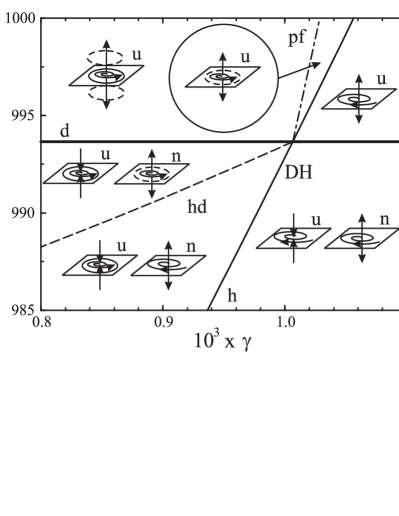
Figure 12: Bifurcations and projections of phase portraits close to the codimension-two domain-Hopf-bifurcation (DH). Thick solid line: spatial instability of the homogeneous steady state (d). Thin solid line: Hopf bifurcation of the homogeneous steady state (h). Dashed line: Hopf bifurcation of the stationary unstable domain (hd). Dash-dotted line: pitchfork bifurcation of limit cycles that stabilizes the homogeneous limit cycle (pf). “u” and “n” denote the planes of uniform and (nonuniform) domain modes, respectively.

the bifurcations and phase portraits near the codimension-two point in which the domain bifurcation and Hopf bifurcation of the homogeneous steady state meet (DH) is shown. The additional branches not shown in fig. 9 are a Hopf bifurcation of the unstable stationary domain leading to an unstable inhomogeneous limit cycle and the pitchfork bifurcation of periodic orbits that stabilizes the homogeneous limit cycle born in the Hopf bifurcation of the homogeneous steady state and which is the origin of another unstable inhomogeneous limit cycle (cf. fig. 5a). Both branches terminate in the DH. The respective phase portraits (insets) depict the dynamics schematically in a projection on the plane spanned by the eigenvectors of the two complex conjugate eigenvalues describing the Hopf bifurcation of the homogeneous fixed point resp. the stationary unstable domain. The third direction describes the subcritical domain bifurcation (spatial mode).

References

- Turing (1952) A. M. Turing, Philos. Trans. R. Soc. London 237, 37 (1952).
- Dewel et al. (1995) G. Dewel, P. Borckmans, A. DeWit, B. Rudovics, J. J. Perraud, E. Dulos, J. Boissonade, and P. DeKepper, Physica A 213, 181 (1995).
- DeWit et al. (1996) A. DeWit, D. Lima, G. Dewel, and P. Borckmans, Phys. Rev. E 54, 261 (1996).
- Meixner et al. (1997) M. Meixner, A. DeWit, S. Bose, and E. Schöll, Phys. Rev. E 55, 6690 (1997).
- Boissonade et al. (1995) J. Boissonade, E. Dulos, and P. DeKepper, in Chemical Waves and Patterns, edited by R. Kapral and K. Showalter (Kluwer Academic, Dodrecht, 1995).
- Valette et al. (1994) D. P. Valette, W. S. Edwards, and J. P. Gollub, Phys. Rev. E 49, R4783 (1994).
- Heidemann et al. (1993) G. Heidemann, M. Bode, and H. G. Purwins, Phys. Lett. A 177, 225 (1993).
- Krischer (1999) K. Krischer, in Modern Aspects of Electrochemistry, edited by B. E. Conway, J. O. Bockris, and R. White (Kluwer Academic/Plenum, New York, 1999), vol. 32, pp. 1–142.
- Krischer et al. (2001) K. Krischer, N. Mazouz, and P. Grauel, Angew. Chem.–Int. Ed. 40, 851 (2001).
- Koper (1996) M. T. M. Koper, in Advances in Chemical Physics, Vol. 92, edited by I. Prigogine and S. A. Rice (Wiley, New York, 1996), pp. 161–296.
- Mazouz et al. (1997a) N. Mazouz, K. Krischer, G. Flätgen, and G. Ertl, J. Phys. Chem. 101, 2403 (1997a).
- Mazouz et al. (1997b) N. Mazouz, G. Flätgen, and K. Krischer, Phys. Rev. E 55, 2260 (1997b).
- Mazouz et al. (1998) N. Mazouz, G. Flätgen, K. Krischer, and I. Kevrekidis, J. Electrochem. Soc. 145, 2404 (1998).
- Flätgen and Krischer (1995) G. Flätgen and K. Krischer, Phys. Rev. E 51, 3997 (1995).
- Grauel et al. (1998) P. Grauel, J. Christoph, G. Flätgen, and K. Krischer, J. Phys. Chem. B 102(50), 10264 (1998).
- Krischer et al. (2000) K. Krischer, N. Mazouz, and G. Flätgen, J. Phys. Chem. B 104, 7545 (2000).
- Strasser et al. (2000) P. Strasser, J. Christoph, W.-F. Lin, M. Eiswirth, and J. Hudson, J. Phys. Chem. A 104, 1854 (2000).
- Christoph et al. (1999a) J. Christoph, R. D. Otterstedt, M. Eiswirth, N. I. Jaeger, and J. L. Hudson, J. Chem. Phys. 110, 8614 (1999a).
- Christoph et al. (1999b) J. Christoph, P. Strasser, M. Eiswirth, and G. Ertl, Science 284, 291 (1999b).
- Kiss et al. (1999) I. Kiss, W. Wang, and J. Hudson, J. Phys. Chem. B 103, 11433 (1999).
- Volkov and Kogan (1969) A. F. Volkov and S. M. Kogan, Phys. Rev. B 11, 881 (1969).
- Bass et al. (1970) F. G. Bass, V. S. Bochkov, and Y. G. Gurevich, Sov. Phys. JETP 31, 972 (1970), [Zh. Eksp. Teor. Fiz. 58, 1814 (1970)].
- Alekseev et al. (1998) A. Alekseev, S. Bose, P. Rodin, and E. Schöll, Phys. Rev. E 57(3), 2640 (1998).
- Meixner et al. (2000) M. Meixner, P. Rodin, A. Wacker, and E. Schöll, Eur. Phys. J. B 13, 157 (2000).
- Meixner et al. (1998) M. Meixner, P. Rodin, and E. Schöll, Phys. Rev. E 58(5), 5586 (1998).
- Bose et al. (2000) S. Bose, P. Rodin, and E. Schöll, Phys. Rev. E 62, 1778 (2000).
- Schimansky-Geier et al. (1991) L. Schimansky-Geier, C. Zülicke, and E. Schöll, Z. Phys. B 84, 433 (1991).
- Schöll (2001) E. Schöll, Nonlinear Spatio-Temporal Dynamics and Chaos in Semiconductors, vol. 10 of Cambridge Nonlinear Science Series (Cambridge University Press, Cambridge, 2001).
- Willebrand et al. (1992) H. Willebrand, T. Hünteler, F.-J. Niedernostheide, R. Dohmen, and H.-G. Purwins, Physical Review A 45(12), 8766 (1992).
- Barelko et al. (1977) V. Barelko, I. Kurochka, A. Merzhanov, and K. Shkadinskii, Chem. Eng. Sci. 33, 805 (1977).
- Zhukov and Barelko (1982) S. A. Zhukov and V. V. Barelko, Sov. J. Chem. Phys. 4, 883 (1982).
- Graham et al. (1993) M. D. Graham, S. L. Lane, and D. Luss, J. Phys. Chem. 97, 889 (1993).
- Middya et al. (1993) U. Middya, M. D. Graham, D. Luss, and M. Sheintuch, J. Chem. Phys. 98(4), 2823 (1993).
- Middya and Luss (1994) U. Middya and D. Luss, J. Chem. Phys. 100, 6386 (1994).
- Annamalai et al. (1999) J. Annamalai, M. Liauw, and D. Luss, Chaos 9(1), 36 (1999).
- Mertens et al. (1993) F. Mertens, R. Imbihl, and A. Mikhailov, J. Chem. Phys. 99, 8668 (1993).
- Mertens et al. (1994) F. Mertens, R. Imbihl, and A. Mikhailov, J. Chem. Phys. 101, 9903 (1994).
- Falcke and Engel (1994) M. Falcke and H. Engel, Phys. Rev. E 50, 1353 (1994).
- Rose et al. (1996) K. Rose, D. Battogtokh, A. Mikhailov, R. Imbihl, W. Engel, and A. Bradshaw, Phys. Rev. Lett. 76(19), 3582 (1996).
- Veser et al. (1993) G. Veser, F. Mertens, A. S. Mikhailov, and R. Imbihl, Phys. Rev. Lett. 71(6), 935 (1993).
- Falcke and Engel (1997) M. Falcke and H. Engel, Phys. Rev. E 56, 635 (1997).
- Elmer (1990) F. J. Elmer, Phys. Rev. A 41, 4174 (1990).
- Seung et al. (1995) K. H. Seung, C. Kurrer, and Y. Kuramoto, Phys. Rev. Lett. 75, 3190 (1995).
- Schebesch and Engel (1996) I. Schebesch and H. Engel, in Self-Organization in Activator-Inhibitor Systems: Semiconductors, Gas–Discharges and Chemical Active Media, edited by H. Engel, F.-J. Niedernostheide, H.-G. Purwins, and E. Schöll (Wissenschaft & Technik-Verlag, Berlin, 1996).
- Vanag et al. (2000) V. K. Vanag, Y. Lingfa, M. Dolnik, A. M. Zhabotinsky, and I. R. Epstein, Nature 406, 389 (2000).
- Battogtokh et al. (1997) D. Battogtokh, M. Hildebrand, K. Krischer, and A. Mikhailov, Phys. Rep. 288, 435 (1997).
- Lima et al. (1998) D. Lima, D. Battogtokh, A. Mikhailov, P. Borckmans, and G. Dewel, Europhys. Lett. 42, 631 (1998).
- Hempel et al. (1998) H. Hempel, I. Schebesch, and L. Schimansky-Geier, Eur. Phys. J. B 2(3), 399 (1998).
- Grauel and Krischer (2001) P. Grauel and K. Krischer, Phys. Chem. Chem. Phys. 3 (2001).
- Otterstedt et al. (1996) R. D. Otterstedt, P. J. Plath, N. I. Jaeger, and J. L. Hudson, J. Chem. Soc., Faraday Trans. 92, 2933 (1996).
- Wacker and Schöll (1994a) A. Wacker and E. Schöll, Z. Phys. B–Condens. Mat. 93, 431 (1994a).
- Bose et al. (1994) S. Bose, A. Wacker, and E. Schöll, Phys. Lett. A 195, 144 (1994).
- Wacker and Schöll (1994b) A. Wacker and E. Schöll, Semicond. Sci. Technol. 9, 592 (1994b).
- Wacker and Schöll (1995) A. Wacker and E. Schöll, J. Appl. Phys. 78, 7352 (1995).
- Schöll (1987) E. Schöll, Nonequilibrium Phase Transitions in Semiconductors (Springer, Berlin, 1987).
- Glavin et al. (1997) B. Glavin, V. Kochelap, and V. Mitin, Phys. Rev. B 56, 13346 (1997).
- Mel’nikov and Podlivaev (1998) D. V. Mel’nikov and A. I. Podlivaev, Semiconductors 32, 206 (1998).
- Gorbatyuk and Rodin (1992) A. V. Gorbatyuk and P. B. Rodin, Solid–State Electron. 35, 1359 (1992).
- Mazouz and Krischer (2000) N. Mazouz and K. Krischer, J. Phys. Chem. B 104, 6081 (2000).
- Li et al. (2001) Y.-J. Li, J. Oslonovitch, N. Mazouz, F. Plenge, K. Krischer, and G. Ertl, Science 291, 2395 (2001).
- Canuto (1993) C. Canuto, Spectral methods in fluid dynamics, Springer series in computational physics (Springer, Berlin, 1993), 3rd ed.
- Hindmarsh (1980) A. C. Hindmarsh, ACM-SIGNUM Newsl. 15, 10 (1980), (lsode is available from the netlib library (netlib@research.att.com)).
- Doedel and Kevernez (1986) E. J. Doedel and J. P. Kevernez, AUTO: A program for continuation and bifurcation problems in ordinary differential equations, Applied Mathematics Report, California Institut of Technology (1986), AUTO is available from http://indy.cs.concordia.ca/auto/.
- Mikhailov (1990) A. S. Mikhailov, Foundations of Synergetics I, vol. 51 of Springer Series in Synergetics (Springer, Berlin, 1990).
- Kerner and Osipov (1994) B. S. Kerner and V. V. Osipov, Autosolitons: a new approach to problems of self-organization and turbulence (Kluwer Academic Publishers, Dordrecht, 1994).
- Guckenheimer and Holmes (1983) J. Guckenheimer and P. Holmes, Nonlinear oscillations, dynamical systems, and bifurcations of vector fields, vol. 42 of Applied Mathematical Sciences (Springer-Verlag, Berlin, 1983).
- Schöll and Drasdo (1990) E. Schöll and D. Drasdo, Z. Phys. B–Condens. Mat. 81, 183 (1990).
- Raizer (1997) Y. P. Raizer, Gas Discharge Physics (Springer, 1997).
- Koper et al. (2001) M. T. M. Koper, T. J. Schmidt, N. M. Markovi, and P. N. Ross, J. Phys. Chem. B in press (2001).