How Fast Elements can Affect Slow Dynamics

Abstract

A chain of coupled chaotic elements with different time scales is studied. In contrast with the adiabatic approximation, we find correlations between faster and slower elements when the differences in the time scales of the elements lie within a certain range. For such correlations to occur, three features are essential: strong correlations among the elements allowing for both synchronization and desynchronization, bifurcation in the dynamics of the fastest element by the change of its control parameter, and the cascade propagation of the bifurcation. The relevance of our results to biological memory is briefly discussed.

Many biological, geophysical and physical problems include a variety of modes with different time scales. The study of dynamical systems with various time scales is important for understanding the hierarchical organization of such systems by investigating the dynamic interactions among modes. Adiabatic eliminationHaken is often adopted for systems with different time scales. If the correlations between modes with different scales are neglected, the fast variables are eliminated and the dynamics of the system is expressed only by the slow variables. The fast variables are then replaced by their averages and noise. In this adiabatic approximation, the characteristics of the dynamics of the fast time scales disappear, and the ”information flow” from fast to slow time scales is only retained as memory terms in a Langevin equation.

The adiabatic approximation is valid when the differences between the time scales are large. However, when the differences are small, correlations between the modes appear, invalidating the approximation. Then, the fast scale dynamics can influence the dynamics of slower variables. Here we investigate under what conditions the faster variables can influence the dynamics of the slower variables. We will show that a dynamical ”information flow” from fast to slow dynamics is possible when a given condition is satisfied. For this, chaos is relevant since it makes possible the amplification of microscopic perturbations to a macroscopic scale. However, in order for the propagation of statistical properties from fast to slow variables to occur, it turns out that two other properties are required: coherence and a cascade of bifurcations.

In the present paper, we investigate how the statistical (topological) properties of the slow dynamics can depend on those of the fast dynamics by adopting a coupled dynamical system with different time scales. To be specific, we choose a chain of nonlinear oscillators whose typical time scales are distributed as a power series. The dynamics of each oscillator is assumed to differ only in its time scale, and thus there are only three control parameters in our model: one for the nonlinearity, one for the coupling strength among oscillators, and one for the difference in time scales.

The concrete form adopted here is as follows: We choose the Lorenz equation as the single oscillator,

$$\left\{\begin{array}[]{ll}\dot{x}=f_{x}(\vec{X})\equiv 10(y-x)\\ \dot{y}=f_{y}(\vec{X})\equiv-xz+rx-y\\ \dot{z}=f_{z}(\vec{X})\equiv xy-\frac{8}{3}z\end{array}\right.$$ (1)

where $\vec{X}\equiv(x,y,z)$. The time scale differences are introduced as

$$T_{i}\frac{d\vec{X}_{i}}{dt}=\vec{F}(\vec{X}_{i}),\ \ \ \ \ T_{i}\equiv T_{1}\tau^{i-1}$$ (2)

where $\vec{F}(\vec{X})=(f_{x}(\vec{X}),f_{y}(\vec{X}),f_{z}(\vec{X}))$. The index of the elements is denoted as $i$ with $i=1,2,,,L=$System size. $T_{i}$ is the characteristic time scale for each element and $\tau$ $(<1)$ is the time scale difference. Using a power series distribution for the characteristic time scales is analogous to the shell model for turbulenceshell . The total time scale difference is given by

$$T_{total}\equiv\frac{T_{L}}{T_{1}}=\tau^{L-1}.$$ (3)

In the present Letter, we adopt the system size $L$ as a control parameter by fixing $T_{total}=100$ and couple neighboring elements diffusively as follows:

$$T_{i}\frac{d\vec{X}_{i}}{dt}=\vec{F}(({\bf E}-{\bf D})\vec{X}_{i}+\frac{1}{2}{\bf D}(\vec{X}_{i-1}+\vec{X}_{i+1}))$$ (4)

$${\bf D}=\left[\begin{array}[]{ccc}d_{x}&0&0\\ 0&d_{y}&0\\ 0&0&d_{z}\end{array}\right],{\bf E}=\left[\begin{array}[]{ccc}1&0&0\\ 0&1&0\\ 0&0&1\end{array}\right]$$

where we chose $d_{y}=0$, $d_{x}=d_{z}=d=0.49$. The Runge-Kutta method was used with a time step size such that the fastest element $\vec{X}_{i}$ is computed with high precision.

Representative examples for the time series of $x_{i}(t)$ are plotted in Fig.1, with $(L,\tau)=$ $(2,100)$ in (a) and $(L,\tau)=$ $(8,1.93)$ in (b). In (a), there is no explicit correlation between the dynamics of the fast time scale at $i=1$ and the slow one at $i=L=2$. On the other hand, there is phase synchronizationPikovsky at various time scales in (b). Here the phase relation between $x_{i}$ and $x_{i+1}$ is anti-phase. The co-variance, given by $\frac{\langle(x_{i}-\langle x_{i}\rangle)(x_{i+1}-\langle x_{i+1}\rangle)\rangle}{\sqrt{\langle(x_{i}-\langle x_{i}\rangle)^{2}\rangle\langle(x_{i+1}-\langle x_{i+1}\rangle)^{2}\rangle}}$, takes a large negative valuecomm-braket . As in the case of coupled phase oscillators with different frequenciesKuramoto , it is natural to expect that correlations appear when the time scale differences $\tau$ become smaller. Due to chaotic instability, however, desynchronization destroys the phase relationship here. Switching between low-dimensional correlated motion and high-dimensional desynchronized motion, known as chaotic itinerancyIkeda-CI ; Kaneko-CI ; Tsuda-CI , appears at various time scales.

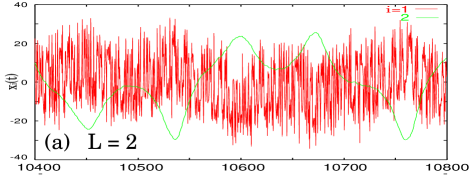
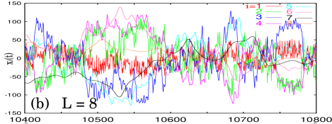
Figure 1: Time series of $x_{i}(t)$. $(L,\tau)=$ $(2,100)$ (a) and $(8,1.93)$ (b). (b) shows correlated motion of elements with various time scales. The colors correspond to the element index. $r=41$ at $1\leq i\leq L$ and $d=0.49$.

Now we will show that the slowest dynamics at $i=L$ can be influenced by the fastest element at $i=1$. In order to do so, we have carried out the following numerical experiment: After the initial transients have died out, at a fixed but otherwise arbitrary point in the temporal evolution of the system, we change the control parameter $r$ of the element $i=1$. Then we examine how the dynamics at $i=L$ is influenced by this change by measuring a statistical property of $x_{L}(t)$.

Fig.2 shows the time series of $x_{i}(t)$ for several values of $\tau$ where the parameter $r$ of element $i=1$ is changed from $41$ to $21$ at $time=180000$. Here $T_{total}=100$ and $(L,\tau)=$ $(2,100)$ (a), $(8,1.93)$ (b), $(10,1.67)$ (c), $(12,1.52)$ (d). In Fig.2(b)-(c), the change in $r$ leads to a novel state with a large amplitude and slow-scale synchronized motion. The characteristic time scale of this state is about $10^{4}$. This is much longer than the time scale of the slowest element $i=L$ which is about $10^{2}$ as can be inferred from Fig.1(a). Hence we find that by modifying the fastest dynamics the dynamics of the slowest element undergoes a qualitative change. Such dependence of the slower dynamics on the control parameter $r$ at $i=1$ is observed only for $6\leq L\leq 12$ (see Fig.2(a) and Fig.2(d)).

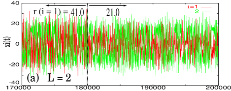
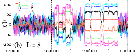
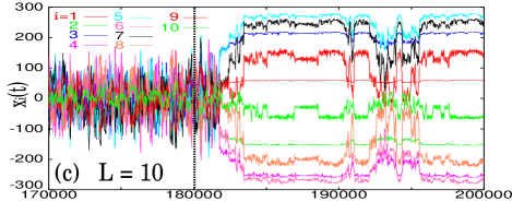
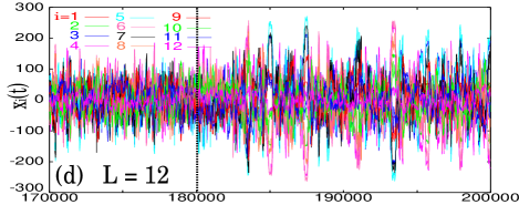
Figure 2: Time series of $x_{i}(t)$. At $time=180000$, the parameter $r$ at $i=1$ is changed from $41$ to $21$. $T_{total}=100$. $(L,\tau)=$ $(2,100)$ (a), $(8,1.93)$ (b), $(10,1.67)$ (c), $(12,1.52)$ (d). In (b)-(c), novel states with coherent large-amplitude motions appear. $d=0.49$.

In order to quantitatively investigate the dependence of the slow time scale on the fast time scale, we low-pass filter $x_{L}(t)$ by averaging over the faster time scale, i.e., $\overline{x_{L}(t)}\equiv\int_{0}^{T_{a}}dt^{\prime}x_{L}(t+t^{\prime})$ and measure the root mean square of the variation of $\overline{x_{L}(t)}$ obtaining the Low-Pass Filtered Root Mean Square (LPF-RMS)commemt1 . In Fig.3(a) we plot the dependence of the LPF-RMS of $x_{L}(t)$ on the control parameter $r$ of the element $i=1$ for various system sizes $L$. For sizes $7\leq L\leq 11$, the LPF-RMS shows a clear increase as $r$ is decreased from $29$. To demonstrate the size dependence, we have plotted the difference of the LPF-RMS of $x_{L}(t)$ between the cases $r=41$ and $21$ for $i=1$ as a function of $L$. As clearly can be seen, the dependence of the slowest element on a parameter of the fastest element only appears for $7\leq L\leq 11$. We have also confirmed that this dependence remains when the system size $L$ is increased, (i.e., by increasing $T_{total}$). Hence the observed dependence is not due to a finite size effect. This dependence exists over finite intervals for the control parameters $r$ of $i=1$, the coupling strength $d$, and the time scale difference $\tau$, not only at a point in the parameter space as would be the case for a phase transition comm-parameter .

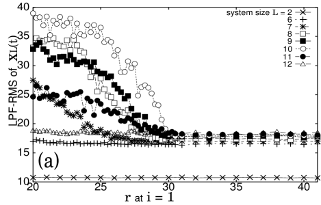
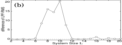
Figure 3: (a) shows the dependence of the Low-Pass Filtered Root Mean Square (LPF-RMS) of $x_{L}(t)$ as a function of the control parameter $r$ of the fastest element $i=1$. $T_{total}=100$. The colors indicate different sets of $(\tau,L)$. Only in the range $7\leq L\leq 11$ the dependence of slow time scales on fast time scales appears. (b) shows the system size dependence of the dependence of the slow time scale on the fast time scale. The ordinate shows the difference of the LPF-RMS of $x_{L}(t)$ between the cases of $r=21$ and $41$ of the element $i=1$.

We also studied a possible dependence of the fast dynamics on the slow dynamics by measuring the dependence of the root mean square of the high-pass filtered value for $x_{1}(t)$, $\overline{\overline{x_{1}(t)}}\equiv x_{1}(t)-\int_{-T_{b}/2}^{T_{b}/2}dt^{\prime}x_{1}(t+t^{\prime})$ on the control parameter $r$ at $i=L$. No such dependence was found, regardless of the values of $(\tau,L)$. Summing up, for values of $\tau$ corresponding to $7\leq L\leq 11$, the slow dynamics depends on the fast dynamics, but the fast dynamics does not depend on the slow dynamics. Hence there is an asymmetry in mutual dependence between the fast and slow variables.

We now study under what condition the slower dynamics depends on the faster dynamics. Based on simulations of the present model for various parameters and also on simulations of the coupled Rössler equation with different time scales, we found the following three requirementsKF-KK-Ross .

First, a strong correlation, either by synchronization or by an anti-phase relationship, between nearest neighbors in the chain is required. When there is no such correlation, the adiabatic approximation for the faster dynamics is valid. For example, for large values of $\tau$, i.e., for $L\leq 7$ in Figs.3), such coherence is not detectable.

Second, a bifurcation in the fastest dynamics is required when a control parameter of the fastest element is changed. In our coupled Lorenz equation with $d=0.49$, the bifurcation from a fixed point to chaos occurs at $r=r_{c}\sim 29$ which corresponds to the bifurcation of a single Lorenz equation at $r\sim 24$. The bifurcation is required to make possible a switching to a different mode of dynamics. However, this second condition by itself is not sufficient for transferring the bifurcated dynamics to slower elements since the control parameters of these elements are not shifted.

For this, a third condition guaranteeing a cascading transfer of the bifurcation from faster to slower elements is required. In the examples of Figs.2, the control parameter of the fastest element $i=1$ is set to $r=21$ allowing for a stable fixed point, while the parameters for the other elements $i>1$ are set to $r=41$ giving chaotic motion. In this case, as can be seen in Figs.2(b)-(c), all elements display chaotic itinerancy between a highly chaotic state and several ordered states around fixed points. As was found in the study of chaotic itinerancy, the switches from one ordered state to another occur irregularly through high-dimensional chaotic motion. In order to distinguish ordered states from chaotic states, we measured the variance over a finite interval, $v_{i}(t;t_{c}(i))\equiv\frac{1}{t_{c}(i)}\int_{0}^{t_{c}(i)}dt^{\prime}(x_{i}(t+t^{\prime})-x_{i}(t+T_{i}+t^{\prime}))^{2}$, where $t_{c}(i)$ is a constant that is scaled as $t_{c0}\tau^{i}$ comm-Lambda . With the help of this quantity, we can roughly roughly estimate whether the element $i$ is in an ordered state or not. If this variance is smaller than its long-term average, $v_{i}(\infty)\equiv lim_{T\rightarrow\infty}\frac{1}{T}\int_{0}^{T}dt^{\prime}(x_{i}(t^{\prime})-x_{i}(T_{i}+t^{\prime}))^{2}$, the element is in an ordered state. From the time series of this variance we found that the intervals where the chain is in the ordered state can be rather long when there is a dependence of the slower dynamics on the faster dynamics (i.e., $7\leq L\leq 11$).

In order to check the residence time distribution of the ordered states, we have classified states with $\frac{v_{i}(t;t_{c}(i))}{v_{i}(\infty)}<0.75$ comm-lamminar as ordered and plotted the results for systems sizes $L=6,8,10,12$ in Fig.4. As can be seen, the residence time distribution follows a power low distribution for $7\leq L\leq 11$ where the dependence of the slower elements on the fastest element is realized. This power law distribution allows for the propagation of bifurcations to ordered states over all elements. It is reminiscent of the energy cascade in fluid turbulence (as described in the shell modelshell ) and the information cascade in a globally coupled mapKaneko94 .

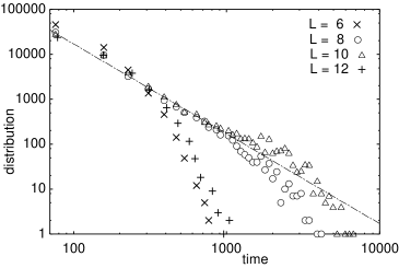
Figure 4: The residence time distribution of ordered states is plotted for $L=6,8,10,12$. $T_{total}=100$. For $L=8,10$, where the propagation from faster to slower elements is observed, a power-law distribution is observed. The dotted line with slope $-2$ is plotted for reference.

When $\tau$ is small, as is shown in Fig.2(d), the chaotic instability is large and the sensitivity to the dynamics of neighboring elements is strongly disturbed by the mixing property. Hence the cascade of bifurcations stops at some element with an intermediate time scale and cannot be propagated to the slowest element.

In conclusion, we have shown that a statistical property of a slower element can successively be influenced by a faster element in a system of coupled chaotic elements with different time scales distributed in a power law. This propagation of information is realized when there is (i) a strong correlation between neighboring elements such as synchronization or anti-phase oscillation, (ii) a bifurcation in the dynamics of the fastest element as its control parameter is changed, and (iii) a cascade propagation of this bifurcation. The mutual dependence of the elements in the chain is asymmetric in the sense that a change of the fastest element can influence the slowest element, but that a change of the slowest element hardly ever influences the fastest element. Since the the three requirements were found to be valid for both the coupled Lorenz equation and the coupled Rössler equation, we believe that it is reasonable to expect that the propagation from faster to slower elements as described in this letter is a universal property of systems of coupled chaotic dynamics with distributed time scales.

Biological systems often incorporate dynamics at various time scales with changes at faster time scales sometimes influencing the dynamics of slower time scales leading to various forms of ‘memory’. A cell can e.g. adapt to an external condition and maintain its memory over a long time span through a change of its intra-cellular chemical dynamics. In a neural system, a fast change in the input is kept as a memory over a much longer time scale when a short-term memory is fixated to a long-term memorybrain . In a similar way, a recently proposed dynamical systems theory for evolution proposes a fixation of a phenotypic change (by bifurcation) to a slower genetic changeKK-Yomo . The present mechanism for the propagation of a bifurcation from faster to slower elements will be relevant for the study of such biological systems and it will be interesting to examine whether the proposed three conditions for the dynamics are satisfied as well. In connection with physics, the possibility of changing the slower dynamics by controlling a faster element through a cascade process will be important for the control of turbulence in general.

The authors would like to thank S.Sasa, T.Ikegami, T.Shibata, H.Chatè, M.Sano, I.Tsuda and T.Yanagita for discussions. They are also grateful to F. Willeboordse for critical reading of the manuscript. This work is partially supported by Grants-in-Aid for Scientific Research from the Ministry of Education, Science, and Culture of Japan (11CE2006).

References

- (1) Haken, Synergetics (Springer 1977)
- (2) M.Yamada and K.Ohkitani, Phys.Rev.Lett. 60, 983 (1988).
- (3) M.G.Rosenblum, A.S.Pikovsky and J.Kurths, Phys. Rev. Lett. 76, 1804 (1996).
- (4) denotes the ensemble average.
- (5) Y.Kuramoto, Chemical Oscillation, Waves, and Turbulence (Springer 1984).
- (6) K.Ikeda, K.Matsumoto and K.Otsuka, Prog. Theor. Phys. Suppl 99, 295 (1989).
- (7) K.Kaneko, Physica 41D, 137 (1990).
- (8) I.Tsuda, Neural Networks 5, 313 (1992).
- (9) LPF-RMS of is calculated as .
- (10) For example, for , this dependence appears when at .
- (11) K.Fujimoto and K.Kaneko, unpublished.
- (12) In the strange attractor of single Lorenz equation, there are two unstable fixed points. When a bifurcation from chaos to fixed point appears, the fixed points are stabilized. In the chaotic state, the dynamics of shows transitions from one of the unstable fixed points to the other at time scale , accordingly takes a large value. On the other hand, in the ordered states these fixed points are stabilized, accordingly takes a small value.
- (13) We set this condition slightly lower than in order to avoid frequent crossing at .
- (14) K.Kaneko, Physica 77D, 456 (1994).
- (15) For a viewpoint on dynamic memory, see e.g., A.Skarda and W.J.Freeman, Behavioral and Brain Sciences 10, 161 (1987). and Tsuda-CI .
- (16) K.Kaneko and T.Yomo, Proc.R.Soc.Rond. 257B, 2367 (2000).