[

Suppression and Enhancement of Diffusion in Disordered Dynamical Systems

Abstract

The impact of quenched disorder on deterministic diffusion in chaotic dynamical systems is studied. As a simple example, we consider piecewise linear maps on the line. In computer simulations we find a complicated scenario of multiple suppression and enhancement of normal diffusion under variation of the perturbation strength. These results are explained by a theoretical argument showing that the oscillations emerge as a direct consequence of the unperturbed diffusion coefficient, which is known to be a fractal function of a control parameter.

PACS numbers: 05.45.Ac, 05.60.Cd, 05.45.Pq, 05.45.-a, 05.40.Ca, 05.45.Df

] Recently there has been growing interest in the field of disordered dynamical systems thus trying to bring together two at first view very different directions of research [3, 4]: Disordered lattices exhibiting quenched (static) randomness are considered as a traditional problem of statistical physics. Hence, in this type of models normal and anomalous diffusion are studied by probabilistic methods being developed in the framework of the theory of stochastic processes [5, 6, 7]. On the other hand, diffusion can also be generated from microscopic chaos in nonlinear equations of motion. This is well-known as the phenomenon of chaotic diffusion in deterministic dynamical systems [8, 9]. Here, methods of dynamical systems theory can be applied for computing deterministic transport coefficients [10, 11, 12]. Disordered dynamical systems represent an interesting combination of both types of models and provide an ideal opportunity to bring these two theoretical approaches together. To our knowledge, only very few cases of such models have been studied so far. Examples include random Lorentz gases for which Lyapunov exponents have been calculated by means of kinetic theory and by computer simulations [13], numerical studies of diffusion on disordered rough surfaces [14] and in disordered deterministic ratchets [15], as well as numerical and analytical studies of chaotic maps on the line with quenched disorder [4, 16].

In this work we will focus on the most simple case in the latter class of models, which are piecewise linear maps defined on the unit interval and acting on the real line by periodic continuation. In case of mixing dynamics, the unperturbed maps exhibit normal diffusion [9, 17, 18, 19, 20]. As first shown in Refs. [4], and as further analyzed in Refs. [16], quenched disorder can change the deterministic diffusive dynamics in these maps profoundly: adding static randomness in form of a local bias with globally vanishing drift leads to dynamical localization of trajectories in a complicated potential landscape. On disordered lattices, this effect is well-known as the Golosov phenomenon [6, 21] thus reappearing in the framework of deterministic dynamics. Here we will consider a second fundamental type of static randomness which is multiplicative and preserves the local symmetry of the model. Consequently, it does not generate subdiffusive behavior [22]. On this basis we study the dependence of the normal diffusion coefficient on two control parameters, which are the strength of the unperturbed diffusion coefficient as well as the perturbation strength [23]. Under variation of these two control parameters we find a complicated scenario for the diffusion coefficient yielding suppression and enhancement of the strength of diffusion as general features. These findings will be explained in terms of a simple theoretical approximation, which is derived from an exact diffusion coefficient formula as obtained within the theory of stochastic processes.

We first define the unperturbed model by the equation of motion

$$x_{n+1}=M_{a}(x_{n})\quad,$$ (1)

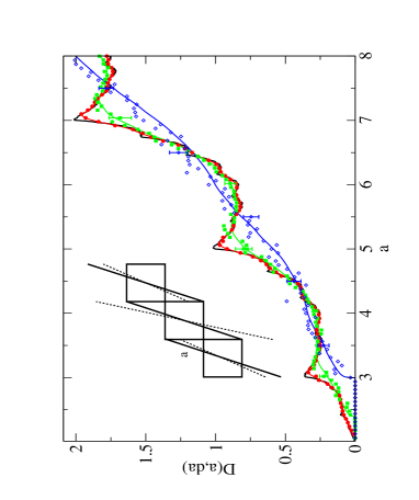
FIG. 1.: Diffusion coefficient $D(a,da)$ for the piecewise linear map shown in the figure. The slope $a$ is perturbed by static disorder of maximum strength $da$ as defined in Eq. (2). The bold black line depicts numerically exact results for the unperturbed diffusion coefficient at $da=0$. Computer simulation results for $da>0$ are marked with symbols, the corresponding lines are obtained from the theoretical approximation Eq. .(5) The parameter values are: $da=0.1$ (circles), $da=0.4$ (squares), $da=1.0$ (diamonds).

where $a\in\hbox{\mb R}$ is a control parameter and $x_{n}$ is the position of a point particle at discrete time $n$. $M_{a}(x)$ is continued periodically beyond the interval $[-1/2,1/2)$ onto the real line by a lift of degree one, $M_{a}(x+1)=M_{a}(x)+1$. We assume that $M_{a}(x)$ is anti-symmetric with respect to $x=0$, $M_{a}(x)=-M_{a}(-x)$. The map we study as an example is defined by $M_{a}(x)=ax$, where the uniform slope $a$ serves as a control parameter. The Lyapunov exponent of this map is given by $\lambda(a)=\ln a$ implying that for $a>1$ the dynamics is chaotic. We now modify this system by adding a random variable $\Delta a(i)$, $i\in\hbox{\mb Z}$, to the slope on each interval $[i-1/2,i+1/2)$ yielding $M_{a}^{(i)}(x)=(a+\Delta a(i))x$. We assume that the random variables $\Delta a(i)$ are independent and identically distributed according to a distribution $\chi_{da}(\Delta a)$, where $da$ is again a control parameter. In the following we will consider two different types of such distributions, namely random variables distributed uniformly over an interval of size $[-da,da]$,

$$\chi_{da}(\Delta a)=(\Theta(da+\Delta a)\Theta(da-\Delta a))/(2da)\quad,$$ (2)

and dichotomous or $\delta$-distributed random variables,

$$\chi_{da}(\Delta a)=(\delta(da+\Delta a)+\delta(da-\Delta a))/2\quad.$$ (3)

Since $|\Delta a|\leq da$, we denote $da$ as the perturbation strength. As an example, we sketch in Fig. 1 the map resulting from the disorder of Eq. (2) as applied to the slope $a=3$. In the absence of any bias, the diffusion coefficient is defined as $D(a,da)=\lim_{n\to\infty}<x_{n}^{2}>/(2n)$, where the brackets denote an ensemble average over moving particles for a given configuration of disorder. An additional disorder average is not necessary because of self-averaging. Note that for locally symmetric quenched disorder and $(a-da)>2$ there is no physical mechanism leading to infinitely high reflecting barriers as they are responsible for Golosov localization [4]. Thus diffusion must be normal, as is confirmed by computer simulations. Hence, the central question is what happens to the parameter-dependent diffusion coefficient $D(a,da)$ under variation of the two control parameters $a$ and $da$.

For the unperturbed case $da=0$ the diffusion coefficient has been computed numerically exactly in Refs. [18, 19]. There it has been shown that $D(a,0)$ is a fractal funtion of the slope $a$ as a control parameter. This function is depicted in Fig. 1, as well as results from computer simulations for different values of the perturbation strength $da$ [24]. As expected, the fractal structure smoothes out by increasing $da$. However, it is remarkable that even for large perturbation strength $da$ oscillations are still visible as a function of $a$ indicating that the original irregularities are very robust against uniform quenched disorder.

Before we proceed to more detailed simulation results we briefly repeat what is known for diffusion in lattice models with random barriers [5, 6, 7, 25]. In the most simple version, the quenched disorder is defined on a one-dimensional periodic lattice with transition rates between neighboring sites $i$ and $i+1$ having the symmetry $\Gamma_{i,i+1}=\Gamma_{i+1,i}\equiv\Gamma_{k}$ for a given random distribution of $\Gamma_{k}$. In this situation an exact expression for the diffusion coefficient has been derived reading [7, 25]

$$D=\{1/\Gamma\}^{-1}l^{2}\quad,$$ (4)

with the brackets defining the disorder average $\{1/\Gamma\}=1/N\sum_{k=0}^{N}1/\Gamma_{k}$ at chain length $N$, and for a distance $l$ between sites. The double-inverse accounts for the physical significance of the fact that the highest barriers dominate diffusion in $d=1$. In other words, the existence of rates with $\Gamma_{k}\to 0$ naturally leads to a vanishing diffusion coefficient $D\to 0$. This scenario is translated to the map under consideration as follows: Eq. (1) can be understood as a time-discrete Langevin equation, $x_{n+1}=x_{n}-\partial V/\partial x(x_{n})$ [4, 9]. In case of quenched disorder, and under proper integration of $M_{a}^{(i)}(x)$, the resulting potential $V(x)$ corresponds to the one of a random barrier model in which the perturbation strength $da$ determines the highest barriers. For the disordered map one may thus naively expect suppression of diffusion reflected in $D(a,da)$ being a monotoneously decreasing function of $da$.

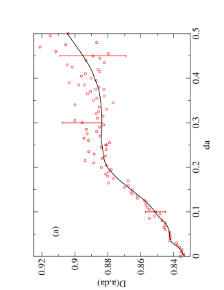
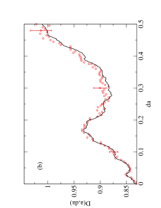
FIG. 2.: Diffusion coefficient $D(a,da)$ as a function of the perturbation strength $da$ at slope $a=6$: (a) disorder distribution Eq. (2), (b) disorder distribution Eq. (3). The circles represent results from computer simulations, the lines are obtained from the theoretical approximation Eq. (5).

To check this hypothesis, we choose fixed values of $a$ corresponding to the two extreme situations of sitting at a local maximum or minimum, respectively, of the unperturbed $D(a,0)$ in Fig. 1. We first focus on the local minimum at $a=6$ for $da\leq 0.5$ with uniform (Fig. 2 (a)) as well as dichotomous (Fig. 2 (b)) disorder. In sharp contrast to the stochastic argument outlined above, in both cases we observe enhancement of diffusion as a function of $da$. Moreover, this enhancement does not appear in form of a simple functional dependence on $da$: In (a), smoothed-out oscillations are visible on smaller scales, whereas in (b) the resulting function is clearly non-monotoneous and wildly fluctuating exhibiting multiple suppression and enhancement in different parameter regions. What happens on larger scales of $da$ is depicted in Fig. 3, where we only show results for dichotomous disorder. As can be seen in Fig. 3 (b), choosing $a$ at a local maximum of $D(a,0)$ leads to suppression of diffusion for $da<1.0$, whereas a local minimum generates enhancement in the same parameter region of $da$. However, in both cases the diffusion coefficient decreases on a larger scale thus recovering qualitative agreement with the expectation from stochastic theory. Indeed, for $(a-da)\to 2$ barriers are formed which a particle cannot cross anymore implying the existence of localization [26].

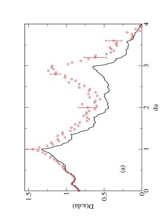
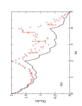
FIG. 3.: Diffusion coefficient $D(a,da)$ as a function of the perturbation strength $da$ for dichotomous disorder Eq. (3) at two different slopes $a$: (a) $a=6$, (b) $a=7$. The circles represent results from computer simulations, the lines are obtained from the theoretical approximation Eq. (5).

To theoretically explain these simulation results, we modify Eq. (4) in a straightforward way such that it can be applied to our disordered deterministic map under consideration. We first note that for uniform transition rates $\Gamma_{k}=const.$ it is $D(\Gamma_{k},l)=\Gamma_{k}l^{2}$. Using this familiar expression for the random walk diffusion coefficient on the unperturbed lattice we rewrite Eq. (4) as $D=\{1/D(\Gamma_{k},l)\}^{-1}$. In case of our map, the transition rates and the distance between sites are both somewhat combined in the action of the slope $a$ as a control parameter. Therefore, the unperturbed diffusion coefficient is correctly rewritten by replacing $D(\Gamma_{k},l)\equiv D(a)$. Up to this point we performed purely formal manipulations. The key question is now what function shall be used for the parameter-dependent diffusion coefficient $D(a)$ in case of deterministic dynamics. Here we propose to identify the function $D(a)$ with the exact, unperturbed deterministic diffusion coefficient previously defined as $D(a,0)$. Providing this information, the exact formula Eq. (4) for stochastic dynamics becomes an approximation which can straightforwardly be applied to deterministic dynamics in disordered systems. If the disorder distributions $\chi_{da}(\Delta a)$ are bounded by the perturbation strength $da$, and if we go into the continuum limit for the random variable, our final result reads

$$D_{app}(a,da)=\left[\int_{-da}^{da}d(\Delta a)\>\frac{\chi_{da}(\Delta a)}{D(a+\Delta a)}\right]^{-1}\quad.$$ (5)

This expression represents the central formula of our letter. The results obtained from it are depicted in Figs. 1 to 3 in form of lines. For small enough $da$ the agreement between theory and simulations is excellent, both for dichotomous as well as for uniform disorder. Surprisingly, for dichotomous disorder the theory even correctly predicts the oscillations for larger $da$, although there are clear quantitative deviations.

We now show that this formula provides a simple physical explanation for the complicated dependence of the diffusion coefficient on the perturbation strength. In case of $da\to 0$, Taylor expansion leads to

$$D_{app}(a,da)=\int_{-da}^{da}d(\Delta a)\>\chi_{da}(\Delta a)D(a+\Delta a)\quad.$$ (6)

We remark that, alternatively, Eq. (6) can be proven for small enough $da$ starting from the precise definition of the diffusion coefficient, and without employing Eq. (5) [27]. In this limit the perturbed diffusion coefficient reduces to an average of the exact diffusion coefficient over the neighborhood in the parameter interval $[a-da,a+da]$ weighted by the respective disorder distribution $\chi_{da}(\Delta a)$. Consequently, if $a$ is chosen at a local minimum the result must be enhancement of diffusion by increasing the perturbation strength, and suppression at a local maximum, respectively [28]. On these grounds it is also clear that the fractal parameter dependence of $D(a,0)$ must reappear in the perturbed diffusion coefficient thus leading to multiple suppression and enhancement on fine scales. In case of dichotomous noise, and if Eq. (6) holds, $D(a,da)$ must be a superposition of two fractals resulting in a new fractal. In case of uniform noise the fractality smoothes out, but is still responsible for the oscillations on a fine scale.

We conclude with a few remarks: (a) It would be important to have a proof of Eq. (5) for dynamical systems, as well as to obtain higher order corrections for explaining the deviations between simulation and theory as visible in Fig. 3. (b) Our results might be important to understand diffusion on a stepped surface with a disordered arrangement of Ehrlich-Schwoebel barriers: As shown in Ref. [29], this problem can be modeled by a potential relief consisting of a combination of random traps and random barriers. Our map provides a deterministic generalization of such a model and particularly enables to study the impact of long-range memory effects on surface diffusion. (c) One could think of applying our approach to systems such as the ones studied in Refs. [14, 15], or to the periodic Lorentz gas [10, 11, 12], which is a model being close to experiments on antidot lattices [30]. Knowing the density-dependent diffusion coefficient in the unperturbed case [31] leads us to predicting local and global suppression of the diffusion coefficient in this model in case of static density fluctuations.

We wish to thank Prof. K.W. Kehr for pointing out to us the existence of Eq. (5), unfortunately, he did not live to see of how much use his hint was for the present work. The author is also grateful to G. Radons, H. van Beijeren, J.R. Dorfman, and T. Tel for helpful discussions.

REFERENCES

- [1]
- [2] Electronic address: rklages@mpipks-dresden.mpg.de.
- [3] “Disordered Dynamical Systems”, conference at the MPIPKS Dresden, organized by G.Radons (March 1998); see http://www.mpipks-dresden.mpg.de/~dds/.
- [4] G. Radons, Phys. Rev. Lett. 77, 4748 (1996); Adv. Solid State Physics 38, 439 (1999).
- [5] J. W. Haus and K. W. Kehr, Phys. Rep. 150, 264 (1987); G. H. Weiss, Aspects and applications of the random walk (North-Holland, Amsterdam, 1994).
- [6] J.-P.Bouchaud and A.Georges, Phys. Rep. 195, 127 (1990).
- [7] K. W. Kehr, in Diffusion in condensed matter, edited by R. H. J. Kaerger, P. Heitjans (Vieweg, Braunschweig, 1998), pp. 265–305.
- [8] T. Geisel and J. Nierwetberg, Phys. Rev. Lett. 48, 7 (1982); M. Schell, S. Fraser, and R. Kapral, Phys. Rev. A 26, 504 (1982).
- [9] S. Grossmann and H. Fujisaka, Phys. Rev. A 26, 1179 (1982); H. Fujisaka and S. Grossmann, Z. Physik B 48, 261 (1982).
- [10] A. Lichtenberg and M. Lieberman, Regular and Chaotic Dynamics, Vol. 38 of Applied Mathematical Sciences, 2nd ed. (Springer, New York, 1992).
- [11] P. Gaspard, Chaos, Scattering, and Statistical Mechanics (Cambridge University Press, Cambridge, 1998); P. Cvitanović et al., Classical and Quantum Chaos (Niels Bohr Institute, Copenhagen, 2001).
- [12] J.R. Dorfman, An Introduction to Chaos in Nonequilibrium Statistical Mechanics (Cambridge University Press, Cambridge, 1999).
- [13] See H. van Beijeren and J.R. Dorfman, Phys. Rev. Lett. 74, 4412 (1995); C. Dellago and H. Posch, Phys. Rev. E 52, 2401 (1995); H. van Beijeren, A. Latz, and J.R. Dorfman, Phys. Rev. E 57, 4077 (1998), Ref. [12], and references therein.
- [14] M. N. Popescu et al., Phys. Rev. E 58, R4057 (1998).
- [15] M. N. Popescu et al., Phys. Rev. Lett. 85, 3321 (2000); C. M. Arizmendi, F. Family, and A. L. Salas-Brito, Phys. Rev. E 63, 061104 (2001).
- [16] H.-C. Tseng and H.-J. Chen, Int. J. Mod. Phys. 13, 83 (1999).; 14, 643 (2000); H.-C. Tseng et al., Physica A 281, 323 (2000).
- [17] R. Artuso, Phys. Lett. A 160, 528 (1991); Physica D 76, 1 (1994); H.-C. Tseng et al., Phys. Lett. A 195, 74 (1994); C.-C. Chen, Phys. Rev. E 51, 2815 (1995).
- [18] R. Klages and J.R. Dorfman, Phys. Rev. Lett. 74, 387 (1995); Phys. Rev. E 59, 5361 (1999).
- [19] R. Klages, Deterministic diffusion in one-dimensional chaotic dynamical systems (Wissenschaft & Technik-Verlag, Berlin, 1996).
- [20] R. Klages and J.R. Dorfman, Phys. Rev. E 55, R1247 (1997).
- [21] Y. G. Sinai, Theor Prob. Appl. 27, 256 (1982); A. O. Golosov, Commun. Math. Phys. 92, 491 (1984).
- [22] Note that what is called suppression of diffusion in Ref. [4] is a mechanism leading to subdiffusion. Here we denote with suppression and enhancement of diffusion the variation of the strength of the normal diffusion coefficient.
- [23] We remark that in previous work on disordered maps only fixed specific parameter values have been chosen where the reduced map corresponds to a Bernoulli shift [4, 16].
- [24] For each point, a maximum of 1,000,000 particles has been iterated up to 50,000 time steps each. Some representative error bars are included in all figures.
- [25] R. Zwanzig, J. Stat. Phys. 28, 127 (1982); B. Derrida, J. Stat. Phys. 31, 433 (1983); S. K. Lyo and P. M. Richards, Phys. Rev. B 32, 301 (1985).
- [26] Simulations have also been carried out for uniform disorder, see Eq. (2). In analogy to Figs. 2 and 3, suppression for up to and global suppression for and over the full range of have been obtained as well, however, with much larger error bars; these results will be presented elsewhere [27].
- [27] R. Klages, to be published.
- [28] Based on this heuristical argument, these phenomena have already been conjectured in Ref. [19], see p. 65.
- [29] K. Mussawisade, T. Wichmann, and K. W. Kehr, Surf. Sci. 412/413, 55 (1998).
- [30] D. Weiss et al., Phys. Rev. Lett. 66, 2790 (1991).
- [31] R. Klages and C. Dellago, J. Stat. Phys. 101, 145 (2000).