Dynamical equations for high-order structure functions, and a comparison of a mean field theory with experiments in three-dimensional turbulence

Abstract

Two recent publications [V. Yakhot, Phys. Rev. E 63, 026307, (2001) and R.J. Hill, J. Fluid Mech. 434, 379, (2001)] derive, through two different approaches that have the Navier-Stokes equations as the common starting point, a set of steady-state dynamic equations for structure functions of arbitrary order in hydrodynamic turbulence. These equations are not closed. Yakhot proposed a “mean field theory” to close the equations for locally isotropic turbulence, and obtained scaling exponents of structure functions and an expression for the tails of the probability density function of transverse velocity increments. At high Reynolds numbers, we present some relevant experimental data on pressure and dissipation terms that are needed to provide closure, as well as on aspects predicted by the theory. Comparison between the theory and the data shows varying levels of agreement, and reveals gaps inherent to the implementation of the theory.

I Introduction

It is well known that the Navier-Stokes (NS) equations of fluid motion can be written in terms of statistical quantities such as the moments of turbulent velocity at several simultaneous spatial points. This statistical reformulation of the dynamic equations introduces extra variables, giving rise to the familiar ‘closure’ problem in hydrodynamic turbulence. If the interest is in the small-scale properties of turbulence, it is more appropriate to obtain equations for the so-called structure functions, which are the moments of velocity increments $\Delta{\mathchoice{{\hbox{\boldmath$\displaystyle u$}}}{{\hbox{\boldmath$\textstyle u$}}}{{\hbox{\boldmath$\scriptstyle u$}}}{{\hbox{\boldmath$\scriptscriptstyle u$}}}}_{r}={\mathchoice{{\hbox{\boldmath$\displaystyle u$}}}{{\hbox{\boldmath$\textstyle u$}}}{{\hbox{\boldmath$\scriptstyle u$}}}{{\hbox{\boldmath$\scriptscriptstyle u$}}}}({\mathchoice{{\hbox{\boldmath$\displaystyle x$}}}{{\hbox{\boldmath$\textstyle x$}}}{{\hbox{\boldmath$\scriptstyle x$}}}{{\hbox{\boldmath$\scriptscriptstyle x$}}}}+{\mathchoice{{\hbox{\boldmath$\displaystyle r$}}}{{\hbox{\boldmath$\textstyle r$}}}{{\hbox{\boldmath$\scriptstyle r$}}}{{\hbox{\boldmath$\scriptscriptstyle r$}}}})-{\mathchoice{{\hbox{\boldmath$\displaystyle u$}}}{{\hbox{\boldmath$\textstyle u$}}}{{\hbox{\boldmath$\scriptstyle u$}}}{{\hbox{\boldmath$\scriptscriptstyle u$}}}}({\mathchoice{{\hbox{\boldmath$\displaystyle x$}}}{{\hbox{\boldmath$\textstyle x$}}}{{\hbox{\boldmath$\scriptstyle x$}}}{{\hbox{\boldmath$\scriptscriptstyle x$}}}})$ over a separation vector, $\textstyle r$. Such an equation for the third-order structure functions is known from Kolmogorov’s pioneering work [1]. This equation is unique because it is exact for homogeneous turbulence. For the so-called longitudinal velocity increment $\Delta u_{r}=u(x+r)-u(x)$, where $u$ is the velocity component along the direction of the separation vector, the third-order structure function is given by

$$\langle\Delta u_{r}^{3}\rangle=-\frac{4}{5}\langle\varepsilon\rangle r,$$ (1)

where $\langle\varepsilon\rangle$ is the average energy dissipation rate. For the third-order structure function of the so-called transverse velocity increment $\Delta v_{r}=v(x+r)-v(x)$, where $v$ is the velocity component transverse to the separation vector, we also have the result

$$\langle\Delta v_{r}^{3}\rangle=0.$$ (2)

The inertial range is defined by $\eta<<r<<L$, where $\eta$ is the Kolmogorov scale and $L$ is the large scale of turbulence. Equations (1) and (2) are both parts of Kolmogorov’s 4/5-ths law.

Recently, Yakhot [2] and Hill [3] have derived dynamical equations for high-order structure functions. Yakhot first derived an equation for the so-called generating function $Z$ from which structure functions of all orders can be obtained by simple differentiation. Hill used a more conventional approach to generate structure function equations. The equations are new, and it is therefore useful to examine if anything further can be learnt about turbulence through them. However, unlike Kolmogorov’s 4/5-ths law, these equations are not closed. Yakhot presents a “mean-field approach” to obtain pressure and dissipation contributions, thereby closing the equations. From these closed equations, it is possible to obtain certain small-scale properties such as the probability density function (PDF) of transverse velocity differences and the scaling exponents of structure functions of all orders. Our goal here is to discuss these new equations for high-order structure functions so as to clarify the closure assumptions, and assess the mean field approach by providing experimental comparisons for theoretical predictions.

Since the equations and the procedure for deriving them are not yet familiar, we summarize them in Sec. II and, for later use, explicitly write them down for structure functions of several orders. Section III introduces the experimental background needed for our purposes, while Sec. IV examines the approximate balance of the equations without closure assumptions—mostly to set the stage for further discussions. We summarize the mean field theory in Sec. V and present in Sec. VI comparisons of its predictions with experimental data on the PDFs of transverse velocity increments and their scaling exponents. Section VII deals more explicitly with the magnitude of dissipation terms, and our conclusions are summarized in Sec. VIII.

II Theoretical background

A Brief review of the relevant equations

Yakhot [2] writes the NS equations in terms of the generating function $Z=<e^{\lambda\cdot\Delta{\mathchoice{{\hbox{\boldmath$\displaystyle u$}}}{{\hbox{\boldmath$\textstyle u$}}}{{\hbox{\boldmath$\scriptstyle u$}}}{{\hbox{\boldmath$\scriptscriptstyle u$}}}}_{r}}>$, where $\Delta{\mathchoice{{\hbox{\boldmath$\displaystyle u$}}}{{\hbox{\boldmath$\textstyle u$}}}{{\hbox{\boldmath$\scriptstyle u$}}}{{\hbox{\boldmath$\scriptscriptstyle u$}}}}_{r}$ is the vector velocity difference between two space points ${\mathchoice{{\hbox{\boldmath$\displaystyle x$}}}{{\hbox{\boldmath$\textstyle x$}}}{{\hbox{\boldmath$\scriptstyle x$}}}{{\hbox{\boldmath$\scriptscriptstyle x$}}}}_{1}$ and ${\mathchoice{{\hbox{\boldmath$\displaystyle x$}}}{{\hbox{\boldmath$\textstyle x$}}}{{\hbox{\boldmath$\scriptstyle x$}}}{{\hbox{\boldmath$\scriptscriptstyle x$}}}}_{2}$ separated by the vector distance $\textstyle r$. The generating function $Z$ is constructed, in the spirit of field theories, so that its Laplace transform gives the probability density function of the velocity differences, and obeys the equation

$${\partial Z\over\partial t}+{\partial^{2}Z\over\partial\lambda_{\mu}\partial r_{\mu}}=I_{f}+I_{p}+D.$$ (3)

Here $I_{f}$, $I_{p}$ and $D$ are the (known) forcing, pressure and dissipative terms respectively, and are given by

$$I_{f} = \langle{\mathchoice{{\hbox{\boldmath$\displaystyle\lambda$}}}{{\hbox{\boldmath$\textstyle\lambda$}}}{{\hbox{\boldmath$\scriptstyle\lambda$}}}{{\hbox{\boldmath$\scriptscriptstyle\lambda$}}}}\cdot\Delta{\mathchoice{{\hbox{\boldmath$\displaystyle f$}}}{{\hbox{\boldmath$\textstyle f$}}}{{\hbox{\boldmath$\scriptstyle f$}}}{{\hbox{\boldmath$\scriptscriptstyle f$}}}}e^{\lambda\cdot\Delta{\mathchoice{{\hbox{\boldmath$\displaystyle u$}}}{{\hbox{\boldmath$\textstyle u$}}}{{\hbox{\boldmath$\scriptstyle u$}}}{{\hbox{\boldmath$\scriptscriptstyle u$}}}}_{r}}\rangle$$ (4)

$$I_{p} = -{\mathchoice{{\hbox{\boldmath$\displaystyle\lambda$}}}{{\hbox{\boldmath$\textstyle\lambda$}}}{{\hbox{\boldmath$\scriptstyle\lambda$}}}{{\hbox{\boldmath$\scriptscriptstyle\lambda$}}}}\cdot\langle e^{\lambda\cdot\Delta{\mathchoice{{\hbox{\boldmath$\displaystyle u$}}}{{\hbox{\boldmath$\textstyle u$}}}{{\hbox{\boldmath$\scriptstyle u$}}}{{\hbox{\boldmath$\scriptscriptstyle u$}}}}_{r}}(\nabla_{2}p({\mathchoice{{\hbox{\boldmath$\displaystyle x$}}}{{\hbox{\boldmath$\textstyle x$}}}{{\hbox{\boldmath$\scriptstyle x$}}}{{\hbox{\boldmath$\scriptscriptstyle x$}}}}_{2})-\nabla_{1}p({\mathchoice{{\hbox{\boldmath$\displaystyle x$}}}{{\hbox{\boldmath$\textstyle x$}}}{{\hbox{\boldmath$\scriptstyle x$}}}{{\hbox{\boldmath$\scriptscriptstyle x$}}}}_{1}))\rangle$$ (5)

$$D = \nu{\mathchoice{{\hbox{\boldmath$\displaystyle\lambda$}}}{{\hbox{\boldmath$\textstyle\lambda$}}}{{\hbox{\boldmath$\scriptstyle\lambda$}}}{{\hbox{\boldmath$\scriptscriptstyle\lambda$}}}}\cdot\langle(\nabla_{2}^{2}\Delta{\mathchoice{{\hbox{\boldmath$\displaystyle u$}}}{{\hbox{\boldmath$\textstyle u$}}}{{\hbox{\boldmath$\scriptstyle u$}}}{{\hbox{\boldmath$\scriptscriptstyle u$}}}}_{r}({\mathchoice{{\hbox{\boldmath$\displaystyle x$}}}{{\hbox{\boldmath$\textstyle x$}}}{{\hbox{\boldmath$\scriptstyle x$}}}{{\hbox{\boldmath$\scriptscriptstyle x$}}}}_{2})-\nabla_{1}^{2}\Delta{\mathchoice{{\hbox{\boldmath$\displaystyle u$}}}{{\hbox{\boldmath$\textstyle u$}}}{{\hbox{\boldmath$\scriptstyle u$}}}{{\hbox{\boldmath$\scriptscriptstyle u$}}}}_{r}({\mathchoice{{\hbox{\boldmath$\displaystyle x$}}}{{\hbox{\boldmath$\textstyle x$}}}{{\hbox{\boldmath$\scriptstyle x$}}}{{\hbox{\boldmath$\scriptscriptstyle x$}}}}_{1}))e^{\lambda\cdot\Delta{\mathchoice{{\hbox{\boldmath$\displaystyle u$}}}{{\hbox{\boldmath$\textstyle u$}}}{{\hbox{\boldmath$\scriptstyle u$}}}{{\hbox{\boldmath$\scriptscriptstyle u$}}}}_{r}}\rangle.$$ (6)

The forcing term in the inertial range is small and may be neglected. The closure of the equation requires a knowledge of $I_{p}$ and $D$. In particular, the advection terms are treated exactly. The pressure term $I_{p}$ contains correlation functions of the form $<(\Delta{\mathchoice{{\hbox{\boldmath$\displaystyle u$}}}{{\hbox{\boldmath$\textstyle u$}}}{{\hbox{\boldmath$\scriptstyle u$}}}{{\hbox{\boldmath$\scriptscriptstyle u$}}}}_{r})_{i}(\Delta{\mathchoice{{\hbox{\boldmath$\displaystyle u$}}}{{\hbox{\boldmath$\textstyle u$}}}{{\hbox{\boldmath$\scriptstyle u$}}}{{\hbox{\boldmath$\scriptscriptstyle u$}}}}_{r})_{j}...(\Delta{\mathchoice{{\hbox{\boldmath$\displaystyle u$}}}{{\hbox{\boldmath$\textstyle u$}}}{{\hbox{\boldmath$\scriptstyle u$}}}{{\hbox{\boldmath$\scriptscriptstyle u$}}}}_{r})_{m}\Delta(\nabla p)>$, and so one requires only the knowledge of the correlation of pressure gradient $increments$ and multipoint velocity increments. The multipoint energy dissipation function $D$ has a structure that depends on details such as the order of the moment considered. As we shall see later, its structure resembles the well-known refined similarity hypotheses of Kolmogorov [4]. In any case, the terms needed for the closure of Eq. (3) are, in principle, well-defined.

In homogeneous, isotropic turbulence, the following transformation of variables is justified: $h_{1}=r$, the separation in the direction parallel to the separation vector; $h_{2}={\lambda.{\mathchoice{{\hbox{\boldmath$\displaystyle r$}}}{{\hbox{\boldmath$\textstyle r$}}}{{\hbox{\boldmath$\scriptstyle r$}}}{{\hbox{\boldmath$\scriptscriptstyle r$}}}}\over r}$, the component of $\lambda$ along $r$; $h_{3}=\sqrt{\lambda^{2}-h_{2}^{2}}$, the component of $\lambda$ in the direction perpendicular the separation vector. In these new variables, Eq. (3) for the generating function becomes

$$\partial_{t}Z+[\partial_{1}\partial_{2}+{d-1\over r}\partial_{2}+{h_{3}\over r}\partial_{2}\partial_{3} +$$ (7)

$${(2-d)h_{2}\over rh_{3}}\partial_{3}-{h_{2}\over r}\partial_{3}^{2}]Z = I_{f}+I_{p}+D,$$ (8)

where $\partial_{i}$ denotes the partial derivative with respect to $h_{i}$. In the new variables, the generating function can be written as

$$Z=<e^{h_{2}\Delta u_{r}+h_{3}\Delta v_{r}}>$$ (9)

where $\Delta u_{r}$ and $\Delta v_{r}$ are the familiar velocity differences in the longitudinal and transverse directions, respectively. The structure functions are then generated by successive differentiation of $Z$ as

$$S_{n,m}\equiv\langle(\Delta u_{r})^{n}(\Delta v_{r})^{n}\rangle=\partial_{2}^{n}\partial_{3}^{m}Z(r)|_{h_{2}=h_{3}=0}.$$ (10)

Let us first focus attention on even-order structure functions for which the dissipation terms are negligible in the inertial range. Multiply Eq. (8) by $h_{3}$, perform $\partial_{3}\partial_{2}^{2n-1}$ of the resulting equation, and take the limit $h_{2}=h_{3}\to 0$. We then have

$${\partial S_{2n,0}\over\partial r} + {d-1\over r}S_{2n,0}-{(d-1)(2n-1)\over r}S_{2n-2,2}=$$ (11)

$$- (2n-1)\langle\Delta p_{x}(\Delta u)^{2n-2}\rangle$$ (12)

$$+ P(1-\cos{r/l_{f}})a_{n,d}S_{2n-3,0},$$ (13)

where $d$ denotes the space dimension, $P$ is the mean energy “pumping” rate, $l_{f}$ is the forcing scale and $a_{n,d}\equiv{2(2n-1)(2n-2)\over d}$. For $n=1$, we obtain the well-known relationship between the second-order longitudinal and transverse structure functions, as

$${\partial S_{2,0}\over\partial r}+{d-1\over r}S_{2,0}={d-1\over r}S_{0,2}.$$ (14)

For $n=2$, Eq. (13) yields a new relation

$${\partial S_{4,0}\over\partial r}+{d-1\over r}S_{4,0}={3(d-1)\over r}S_{2,2}-3\langle(\Delta p_{x})(\Delta u)^{2}\rangle,$$ (15)

which is exact in the case of incompressible, isotropic turbulence in the limit of zero viscosity. To extract further information from this equation, one has to invoke some closure. From now on, we consider only three dimensional turbulence unless specified otherwise. If the pressure term is small in the inertial range (a consideration to which we will return momentarily), we obtain

$${\partial S_{4,0}\over\partial r}+{2\over r}S_{4,0}\approx{6\over r}S_{2,2}.$$ (16)

Following this same procedure, it is now easy to write down a sixth order equation with $n=3$ in Eq. (13). Neglecting the pressure term again, we obtain

$${\partial S_{6,0}\over\partial r}+{2\over r}S_{6,0}\approx{10\over r}S_{4,2}.$$ (17)

In a similar manner, we can extract two additional relations for fourth and sixth orders. Their corresponding approximate forms (again neglecting pressure contributions) are

$${\partial S_{2,2}\over\partial r}+{4\over r}S_{2,2}\approx{4\over 3r}S_{0,4}$$ (18)

$${\partial S_{2,4}\over\partial r}+{6\over r}S_{2,4}\approx{6\over 5r}S_{0,6}.$$ (19)

Equations (16)-(19) were also derived by Hill [3] by making a convenient change of variables so that the scale-dependent parts of the equation can be separated from the position-dependent parts and by eliminating the position-dependence in the presence of homogeneity. For the particular case of isotropy, Hill developed a matrix algorithm for solving the system of equations that determined all components of the tensorial structure function of a given order. The dynamical equations obtained for homogeneous and isotropic turbulence confirm Yakhot’s results. Hill’s formulation provides an additional useful fact that there are exactly two equations relating fourth-order structure functions, namely Eqs. (16) and (18). For the sixth order, his procedure shows that there are $three$ equations relating the non-zero components of structure functions, and the third equation is easily generated. Again without the pressure terms, this remaining sixth-order equation is

$${\partial S_{4,2}\over\partial r}+{4\over r}S_{4,2}\approx{4\over r}S_{2,4}.$$ (20)

Equations (16)-(20) are relationships among different components of structure function tensor of the same order. Without pressure terms, they form a closed set for each even order.

Hill’s procedure is convenient for writing down the equations for odd-order structure functions. The equation for the third-order is the well-known Kolmogorov equation (see Eqs. (1) and (2)), which need not be written down again. There are three equations for the fifth order, which, again without pressure and dissipation terms, are

$${\partial S_{5,0}\over\partial r}+{2\over r}S_{5,0}\approx{8\over r}S_{3,2};$$ (21)

$${\partial S_{3,2}\over\partial r}+{4\over r}S_{3,2}\approx{8\over 3r}S_{1,4};$$ (22)

$${\partial S_{1,4}\over\partial r}+{6\over r}S_{1,4}\approx 0.$$ (23)

The $\approx$ symbol in these equations has to be treated with greater caution than for the even-order case because the equations for odd-order structure functions contain dissipation terms as well, see [2]. Therefore the approximation implied in the equations (21)-(22) implies the neglect of dissipation terms as well. We will assess this additional aspect in Sec. VII, but can see by inspection that the approximations cannot be correct for at least the last equation of the above set. It contains only one component of the fifth order structure function, $S_{1,4}$, which, when estimated using Kolmogorov’s K41 scaling [5], shows that the the approximation Eq.(23) cannot hold true.

A further discussion of these equations, and the of degree to which they may be reasonable, requires some contact with experiments. It is therefore necessary to introduce some basic experimental details at this stage before resuming the discussion of the theory.

III Experimental conditions

The velocity data were acquired by means of a $\times$-wire probe mounted at a height of about 35 m above the ground on a meteorological tower at the Brookhaven National Laboratory. The hot wires were about 0.7 mm in length at 5 $\mu$m in diameter. They were calibrated just prior to being mounted on the tower, and operated on DISA 55M01 constant-temperature anemometers. The frequency response of the hot wires was typically good up to 20 kHz. The voltages from the anemometers were low-pass filtered and digitized. The low-pass cutoff was never more than half the sampling frequency $f_{s}$. The sampling rate was adequate to resolve most of the scales, including dissipative ones. The voltages were converted to velocities in a standard way through the standard nonlinear calibration procedure. The mean wind velocities, roughly constant over the duration of a given data set, ranged between 5 and 10 ms^-1 in the entire series. The usual procedure of surrogating time for space (“Taylor’s hypothesis”) was used to obtain the mean dissipation rate $\langle\varepsilon\rangle$ and an estimate for the Kolmogorov scale $\eta$.

The relevant details of the data analyzed here are given in [6, 7]. Briefly, the Taylor microscale Reynolds number is 10,680, the large scale $L$ is about 42 m, Kolmogorov scale $\eta$ is 0.44 mm, the scaling range according to the linear part in the third-order structure function is conservatively between 0.01 m and 0.2 m (although it could be stretched in either direction by factors of 2). This will be regarded as the operational definition of the inertial range.

The theoretical development discussed here is meant for locally isotropic turbulence appropriate to asymptotically large Reynolds numbers. The present measurements are indeed at large enough Reynolds numbers, but it is not obvious that the small scales are isotropic. Indeed, we have used similar data before [8, 9] to extract anisotropic parts of the structure functions by performing the SO(3) decomposition. Thus, a few explanatory words regarding the degree of isotropy are appropriate here.

Figure 1 shows the longitudinal spectral density $E_{11}$ and the transverse spectral density $E_{22}$ for one of the data sets. If strict isotropy prevails in the inertial range, the ratio $E_{22}/E_{11}$ should be 4/3. The data show that the ratio, while varying slowly in the inertial range from a somewhat smaller value than 4/3 to a somewhat larger value, is not far from being 4/3. Similarly, for third-order structure functions, we have the exact result [10] that the ratio $S_{1,2}/S_{3,0}$ should be 1/3. Measurements show that this ratio, which is indeed reasonably constant in the inertial range, has a magnitude of about 0.42 (see Fig. 2). There is undoubtedly some degree of anisotropy in the inertial range, and so the conclusions are to some degree affected by this artifact. To pursue this issue further, we note that $S_{3,0}$ has the expected value of 4/5, and $S_{0,3}$, which should be zero exactly for the isotropic case, is of the order of 0.1 $S_{3,0}$. The anisotropy is thus not large, and the transverse component is perhaps the more anisotropic. This conclusion is consistent with [9, 11].

In summary, then, we regard for present purposes the departures from isotropy to be relatively small in the inertial range, especially for even orders, and expect that the results will not be qualitatively affected by their presence. The quantitative effect is not easy to ascertain, though it is likely to be modest from the considerations just cited.

IV The balance of the approximate equations

Using the experimental data just described, we calculate the left-hand side (LHS) and right-hand side (RHS) of each approximate equation of Sec. II, and obtain the relative size of the difference (LHS - RHS)/LHS; for even orders, this difference is an estimate of the magnitude of the neglected pressure terms. Figures 3, 4, 5, 6 and 7 display the results for Eqs. (16), (17), (18), (19) and (20), respectively. The absolute value of the relative difference is also shown in each case. In the inertial range, all four equations seem to balance reasonably well without the pressure terms, their contribution being of the order of 10$\%$ of the LHS for all equations, growing larger as $r$ becomes larger as well as smaller. To that extent, the closure of Eqs. (16)-(20) in the inertial range seems to be approximately justified.

The situation with respect to odd-order structure functions is somewhat different. Odd-order moments do not converge as well as even-order moments do, and so we may expect significantly more scatter in experimental plots. The terms for the three equations (21)-(23) are shown in Figs. 8-10. Despite the large scatter, it is reasonably clear that the relative difference of LHS and RHS in Fig. 8 is of the order of $20-30\%$ in the inertial range. In Fig. 9, the relative difference is perhaps larger, up to $50\%$ at places. For Eq. (23), as was expected and remarked upon earlier, there is no balance at all (see Fig. 10).

Before examining these issues, it is worth commenting on the intriguing observation that the pressure effects are small in the inertial range at least for even-order structure functions. This feature suggests that the operating physics there might have some relation to that of the forced Burgers equation. It further suggests that the pressure terms may become effective only in the dissipation range (and also for large scales, which we will not consider here). It is reasonable to suppose that vortex structures (qualitatively like wing-tip vortices) are generated as soon as the pressure terms are activated. Perhaps the small-scale vortex tubes (also called worms, see [12, 13]), are a result of this effect. Clearly, the validity of the pressureless physics is limited because the scaling exponents saturate for the forced Burgers equation, whereas there is no evidence that the saturation occurs for three-dimensional turbulence (at least for moments up to order ten; see Sec. VI). In any case, the smallness of pressure terms suggests that the intercomponent energy transfer (for which they are responsible) is small, and that any remnant anisotropies at the large-scale end of the inertial range tend to persist, or at least not diminish rapidly, as the scale size decreases through the inertial range. There is growing evidence from other measurements that this might indeed be so [9, 14].

V A mean field theory

The previous section has shown that the imbalance in the approximate equations for even-order structure functions, caused entirely by the neglect of pressure terms, is of the order 10%. The imbalance is larger for odd-orders, for which it is to be remembered that dissipation terms are also important. Thus, ignoring pressure and dissipation terms is not an option in general, and it is clear that one must make a plausible theory for them. This has been attempted in the mean field theory of [2]. Though our interest and contributions are primarily in the experimental assessment of the theory, it is helpful to provide here a summary of the theory itself—if only to clarify the motivation for the experimental tests performed. We shall focus on the essence of the physical arguments, rather than on analytical details.

A General remarks

Mean field theories provide approximate means of describing a thermodynamic system by supposing that each ‘particle’ in a many-body system moves in the ‘mean’ field of all other particles in the system. This is opposite to the situation in which only nearest neighbor interactions matter. More formally, attribute to the system an order parameter $\phi$ that is zero when the system is ordered and becomes increasingly non-zero with increasing disorder. If the fluctuations in the order parameter are small, then it may be replaced by a spatially uniform average value. The mean field approximation implies infinite range interactions; while this cannot be realized in practice, the order parameter in many thermodynamic systems could become arbitrarily small as the temperature approaches a phase transition value, $T_{c}$. The Ginzburg-Landau theory makes use of this feature to propose a description of the free energy and to derive critical exponents at phase transitions. In general terms, the free energy $F(\phi,T)$ is expanded in powers of $\phi$ as

$$F=F_{0}+A\phi+B\phi^{2}+C\phi^{3}+\dots$$ (24)

where $A$, $B$ and $C$ are functions of $T$. Near the critical point in the $T$-space, where $T\rightarrow T_{c}$, the expansion can be truncated at the lowest order terms in $\phi$. The expansion then provides a qualitative description of the thermodynamic processes; in practice, this mean field approach may work even far from the critical point.

Strictly speaking, a mean field theory may not apply to turbulence where quantities such as the free energy and order parameter cannot be defined unambiguously. In Yakhot’s theory, the idea is carried over qualitatively by identifying a small parameter in some regime and expanding other dependent quantities around that small parameter. The ‘phase transition’ considered is the change of sign in energy flux that occurs in going from two-dimensional ($2d$) to three-dimensional ($3d$) turbulence. It is understood from Kolmogorov’s equation for the third-order structure function that the energy transfer is from the small to the large scale in $2d$ turbulence, and vice versa in $3d$ turbulence. It is assumed that this change is continuous, changing sign at some critical dimension $d_{c}$—analogous to the critical temperature $T_{c}$ in thermodynamic phase transitions. In $2d$ turbulence, the dissipation is negligible for high Reynolds numbers (because the energy ultimately concentrates in the large scale). In $3d$ turbulence, on the other hand, the dissipation is the key to energy transfer from large to small scales. The hope, then, is that both pressure and dissipation can be expanded in terms of a small parameter in the vicinity of $d_{c}$.

B The pressure terms

In turbulence dynamics, transverse structure functions do not participate in energy transfer. Yakhot therefore regards the fluctuations in the transverse velocity increment $\Delta v_{r}$ as small—in effect, if not in actual fact. It is known from numerical simulations [15] as well as experiments [16] of the inverse cascade in $2d$ turbulence that $\Delta v_{r}$ is almost exactly gaussian. The absence of intermittency makes it plausible to regard the fluctuations as “small”. We shall therefore consider the $2d$ case briefly.

The key step for further analysis is the introduction of a conditional expectation of the pressure gradient increment for a fixed value of $\Delta u_{r}$, $\Delta v_{r}$ and $r$ as

$$\langle\partial_{y}p(x+r) - \partial_{y}p(x)|\Delta u_{r},\Delta v_{r},r\rangle$$ (25)

$$\approx \sum_{m,n}\kappa_{m,n}(r)(\Delta u_{r})^{m}(\Delta v_{r})^{n}.$$ (26)

This is related to the needed correlations in $I_{p}$ which is of the form

$$\langle (\partial_{y}p(x+r)-\partial_{y}p(x))(\Delta u_{r})^{p}(\Delta v_{r})^{q}\rangle$$ (27)

$$= \int\langle\partial_{y}p(x+r)-\partial_{y}p(x)|\Delta u_{r},\Delta v_{r},r\rangle\Delta u_{r}^{p}\Delta v_{r}^{q}$$ (28)

$$\times P(\Delta u_{r},\Delta v_{r},r)d(\Delta u_{r})d(\Delta v_{r})d^{3}r.$$ (29)

The use of the conditional expectation provides a tool for expanding the pressure terms in terms of the “small quantity” $\Delta v_{r}$. Now, in the spirit of the Ginzburg-Landau expansion, only the lowest order terms in $\Delta v_{r}$ are retained (corresponding to $\Delta u_{r}\Delta v_{r}$ and $\Delta v_{r}$). The prefactors of the expansion are constrained by the incompressibility condition and by the dimensionality of space.

By substituting in Eqs. (9)-(11) the pressure term derived from the conditional expectation value, and assuming the exponents to be given by from Kolmogorov’s K41 scaling arguments [5], Yakhot concludes that the high-order even moments are consistent with gaussianity. The argument is circular but internally consistent. The gaussianity of the transverse increment $\Delta v_{r}$ is then deduced from Eqs. (13)-(15). This is in excellent agreement with the results of numerical simulations of [15]. Thus, we might conclude that a plausible mean field expression for the pressure contribution exists for $2d$.

The next crucial assumption of the theory is that the above form of the mean field approximation is applicable also for $3d$ turbulence. The rationale is not easy to articulate, especially because, unlike in $2d$ turbulence, the PDFs of $\Delta v_{r}$ possess stretched-exponential tails in $3d$ turbulence [19]. We shall provide some statements of mild justification subsequently, but emphasize that the validity of this assumption has to rest on the basis of the agreement, or lack thereof, with experiments.

C The small parameter and the dissipation term

We need to consider the dissipation term before turning to experiments again. In the inverse cascade range in $2d$ turbulence the dissipation term $D$ can be set to zero because the flow evolution is towards larger and larger scales. However, $D$ is central in $3d$ turbulence, and it is known that dissipation fluctuations are immense at high Reynolds numbers [17]. The objective in a mean field approach is to locally smooth out the fluctuations, through some procedure such as Obukhov’s [18]. For closure, there is a need to relate this coarse-grained dissipation field to velocity fluctuations, analogous to that employed in Kolomogorov’s refined similarity hypotheses [4, 20]. Yakhot’s theory is similar in spirit but the details are different, as we shall illustrate.

Let us denote a coarse-grained velocity field for a given spatial scale $r$ by $V_{r}$. This will be assumed to be the same as $\Delta v_{r}$. Certain one-loop calculations of Yakhot and Orszag [21] give the effective viscosity as

$$\nu_{r} \approx (d-d_{c})^{1\over 3}N(\varepsilon_{r}r^{4})^{1\over 3}$$ (30)

$$\approx V_{r}^{2}\tau_{r}+higher~{}order~{}nonlinear~{}terms$$ (31)

where $N$ is a constant that depends weakly on the space dimensionality, $d$, and $\varepsilon_{r}$ is the dissipation rate coarse-grained on the scale $r$. If we ignore nonlinear terms, this equation provides a natural definition of $\tau_{r}$, the characteristic time for the field $V_{r}$.

There is no obvious justification for ignoring the higher order nonlinear terms which, in $3d$ turbulence, are typically $O(1)$, nor in assuming that $\tau_{r}$ is small compared to $V_{r}/r$. However, if we assume that the theory can be analytically continued into non-integer dimensions between 2 and 3, a suitable small parameter can be generated as follows. The time scale characterizing the interaction of a scale $r$ with all other scales less than $r$ is the so-called eddy turn-over time, or the time taken for energy transfer to occur between $r$ and the Kolmogorov scale $\eta$. One may use K41 to estimate this time scale. The process of energy transfer can be thought to consist of two distinct steps, one involving nonlinear transfer across scales without any pressure effects, and another involving the relaxation due to pressure effects. In $3d$ turbulence, these two steps are parts of the same simultaneous process, so the time scales associated with them cannot be separated. But, if, as one approaches $d_{c}$, it is increasingly true that the pressure effects are small except when scales of the order $\eta$ are reached, the two time scales involved could become disparate, and the relaxation due to pressure terms enters the picture only at the smallest scale and can therefore be assumed to be fast. Then the dimensionless ratio $q_{r}\equiv{\tau_{r}/\theta_{r}}$, where $\tau_{r}$ is the time scale for relaxation effects and $\theta_{r}$ is the time scale for energy transfer, would be a small parameter.

Using this basic idea and his one-loop calculations [21], Yakhot deduces the following results:

$$d_{c}=2.56,~{}q_{r}\approx(d-d_{c})^{1/2},~{}V_{r}\approx(d-d_{c})^{-1/6},$$

and so forth. The notion of a critical dimension is not new (see [22]), though the estimates for it in [2] and [22] are substantially different. The precise numbers and powers in the above equation depend in detail on the approximation made to compute them, and are presumably not final; they cannot, in any case, be verified experimentally near the critical dimension. Here, we merely wish to draw upon the general idea of a critical dimension near which a small parameter can be defined, and in whose vicinity the energy piles up (as shown by the last of the three relations above: the energy is being pumped at a constant rate but is being transferred neither upscale as in $2d$ nor downscale as in $3d$). These ideas allow Yakhot to truncate the effective viscosity and write the dissipation $\varepsilon_{r}$ in terms of the lowest order terms in terms of the coarse-grained velocity field in the vicinity of $d_{c}$:

$$\varepsilon_{r}\approx-{1\over 2}{\partial\over\partial r_{i}}[V_{ri}V^{2}_{rj}(1+O(d-d_{c}))]$$ (32)

Perhaps two additional remarks might be usefully made. First, the coarse-grained velocity fluctuations become very large as the critical dimension is approached, yet it may seem that the mean field approximation proposed for pressure terms assumes that fluctuations are small. To avoid confusion, it is important to keep in mind the distinction between fluctuations in longitudinal and transverse velocity increments. The velocity scale that blows up is related to energy transfer, and hence the longitudinal velocity component, but the component whose fluctuations are supposed to remain small is the transverse velocity. The sense in which those fluctuations are small is unclear (because they too are intermittent in $3d$, see [19]), but the fact remains that it takes no part in energy transfer and so its $effects$ are thought to be “small” in some rough sense. Since the pressure effects are small, the intercomponent energy transfer is inhibited, and so, once fluctuations in $\Delta v_{r}$ are small at some scale, they will presumably remain small at others as well. Secondly, in order to be able to truncate the energy dissipation, the higher order viscosity terms have to decay faster than the rate of blow-up of velocity fluctuations. This is indeed the case above.

Now, keeping in the mind the symmetries of the NS equations, the simplest form for the $V_{r}$ contributions to the dissipation rate is

$$\langle\varepsilon\rangle\approx c(d)\Delta u_{r}\Delta v_{r}{\partial\Delta v_{r}\over\partial r}$$ (33)

The coefficient $c(d)$ must reflect the change in going from $2d$ to $3d$ (zero dissipation to finite dissipation). This may not be a smooth change (as in second-order phase transitions) because $c(d_{c})$ could well be singular (as in first-order phase transitions). Yakhot assumes, however, that it is $O(1)$ for $d-d_{c}>0$. Then $D$ takes on a form similar to Kolmogorov’s refined similarity hypothesis, relating $\langle\varepsilon_{r}\rangle$ with the third-order longitudinal structure function:

$$D \approx c(d)h_{3}\partial_{h_{2}}\partial_{h_{3}}\partial_{r}Z$$ (34)

$$\approx c(d)h_{3}^{3}\langle\Delta u_{r}\Delta v_{r}{\partial\Delta v_{r}\over\partial r}e^{h_{2}\Delta u_{r}+h_{3}\Delta v_{r}}\rangle$$ (35)

$$+ terms~{}neglected.$$ (36)

This enables the closure to be complete.

A non-trivial difficulty is the testing of the theory in non-integer dimensions near $d_{c}$. At present, the consequences of the theory can only be tested in $2d$ or $3d$. The extrapolation to non-integer dimensions is not an intrinsic limitation of the theory, but reflects the lack of experimental ingenuity at present. It must, however, be noted that in shell models where an interaction parameter can be tuned to change the direction of energy transfer, one can make more reasonable contact with the theory. Such comparisons have been attempted recently [24] and the results are encouraging. We have already noted that the conclusions of the theory are consistent with experiments and simulations of $2d$ turbulence. We shall examine in the rest of the paper the extent to which the predictions of the theory are applicable also to $3d$.

VI Comparison of the theory with measurements in three-dimensional turbulence

A Probability density function of transverse velocity increments

When the forms of $I_{p}$ and $D$ from previous sections are substituted into the full structure function equations, one can generate the following equation for the PDF of transverse velocity increments $P(\Delta v_{r},r)\equiv P(V,r)$:

$${\partial P\over\partial r}+{1+3\beta\over 3r}{\partial\over\partial V}VP-\beta{\partial\over\partial V}V{\partial P\over\partial r}=0.$$ (37)

Here $\beta\propto c(d)$. This equation is linear and can be solved in principle, but the solution has no simple analytic form. (For some discussion of this aspect, see [23].) For small $V$, however, the equation admits a solution of the type $r^{\kappa}F(V/r^{\kappa})$ with

$$P(V=0,r)\propto r^{-\kappa},$$ (38)

where, from Yakhot’s theory,

$$\kappa\equiv{1+3\beta\over 3(1-\beta)}\approx 0.4$$ (39)

and $\beta\approx 0.05$. Using the fact that the variance $\sigma_{V}$ of $V$ is expected to vary as $r^{0.35}$ (see [6]), we have the result

$$P({V\over\sigma_{V}}\rightarrow 0,r)\equiv\sigma_{V}P(V\rightarrow 0,r)\approx r^{-0.05}.$$ (40)

We shall now test these predictions.

The precise measurement of the peak value of the PDFs from the data must be done carefully because it is sensitive to the bin width chosen around $V=0$. In our measurements, the bin width around $V=0$ was gradually refined until the PDF value at the origin no longer depended on the bin size. Figure 11 shows that $P(V\rightarrow 0)$ at $r\approx 100\eta$ asymptotes to a value of 0.64. The sharp ascent of the numbers for very small values of the bin width is an artifact of the extreme narrowness of the bin width, which results in false values when normalizing. The procedure was repeated for several values of $r$. Figure 12 shows the properly normalized PDF values for $V=0$ for different scales $r$ ranging from the Kolmogorov scale $\eta$ to the large scale $L$. The scaling exponent for this quantity is $\approx-0.065$ in the inertial range, numerically about 25$\%$ larger than the theoretical value of -0.05. With this experimentally derived scaling exponent, we can evaluate that $\beta\approx 0.058$ compared to the theoretical value of $0.05$, a 16$\%$ difference. Figure 13 also shows that the form $r^{\kappa}P(V/r^{\kappa})$ is essentially constant for small $V$.

One can obtain the form of $F$ for large $V$ by a steepest descent approximation (see [23] for more details). The result from [2] is

$$F\propto{1\over\sqrt{\Omega(r)}}\exp\Big{(}-{(\ln\xi)^{2}\over\Omega(r)}\Big{)},$$ (41)

where $\xi=VL^{\beta\kappa\over\beta-1}/r^{\kappa(1-2\beta)/1-\beta}$, and $\Omega(r)={\beta\kappa\over(1-\beta)^{2}}|\ln(r/L)|$. (The corresponding expressions in [2] are printed incorrectly.) The prefactor of Eq. (41) is possibly $r$-dependent. Equation (41) can be re-written as

$$(-\Omega(r)\ln(P(V,r)r^{\kappa}\sqrt{\Omega(r)})^{0.5}\propto\ln(\xi).$$ (42)

Figure 14 shows plausible linear behaviors for the tails of the PDF in the proposed logarithmic units of Eq. (42). There is, however, evidently still some $r$-dependence that precludes their collapse. We recall that corrections to steepest descent approximations are often logarithmic, but are difficult to calculate here analytically. We assume a dependence of the form $(\ln(r/L))^{\gamma}$ for the proportionality factor. Figure 15 shows a replot of the data with the additional factor of $(\ln(r/L))^{2}$ multiplying the PDF. The exponent $2$ was chosen because it collapses the data best in the inertial range. (The one separation distance that does not collapse belongs to the dissipation range.)

Our main conclusion so far is that the mean field models for pressure and dissipation terms provide a way for closing the PDF equation, and for solving it for the limiting situations. The prediction is that, to first approximation, the tails of the PDF of $\Delta v_{r}$ are lognormal. The experimental data suggest that this might be so, but that an $r$-dependent contribution is missing. It is at present not clear whether this missing aspect is merely a correction to asymptotics, or corresponds to additional terms in the mean field expansion, or is even more fundamental.

B The scaling exponents and the prospect of their saturation

Seeking the solution to Eq. (37) under the K41 constraint for the third-order structure functions and assuming $S_{0,n}\propto r^{\zeta_{n}}$, Yakhot obtained the following formula for the structure function exponents:

$$\zeta_{n}={n(1+3\beta)\over 3(1+\beta n)}.$$ (43)

Table I and Fig. 16 show the calculated exponents and compare them with those obtained from the Direct Numerical Simulations, or DNS, data [25] as well as experiments. The agreement is good for all orders, perhaps slightly better for the DNS data for high order exponents.

Using probability density functions to define the statistical quantities, we have (putting $U=\Delta u_{r}$) the conditional expectation value of $V^{2}$ for a fixed value of $U$, $Q_{2}(U)$, as

$$S_{2n-2,2}=\int P(U)U^{2n-2}Q_{2}(U)dU.$$ (44)

See Sec. IV of [2]. The Kolmogorov scaling will hold (by dimensional arguments) for $Q_{2}(U)\propto U^{2}$. On the other hand, saturation of exponents, $\zeta_{2n}\rightarrow$ constant as $n\rightarrow\infty$, is possible for $Q_{2}(U)\propto U^{\delta}$ for $\delta<2$ and $U$ large. We present the conditional statistical quantity $Q_{2}(U)$ as a function of $r$ in Fig. 17. It is not clear if the trend for large $U$ is in agreement with the saturation condition. There is a very small range of $U$ towards the tails which seems to vary as ${U^{2}/\ln(U^{2})}$ but this is not conclusive. There might also be the influence of anisotropy in the PDFs, as is evident, for example, in the asymmetry of the joint PDFs, which in turn could change the nature of the tails of the conditional statistics.

VII Remarks on the magnitude of dissipation terms

It is helpful to recall that the full form of the equation relating even order transverse moments to mixed moments of the same order in $3d$ is

$${\partial S_{2,2n}\over\partial r}+{2+2n\over r}S_{2,2n} = {2+2n\over 2n+1}{S_{0,2n+2}\over r}$$ (45)

$$- 2n\langle{\cal P}_{yv}\Delta u(\Delta v)^{2n-1}\rangle,$$ (46)

where ${\cal P}_{yv}\equiv\partial_{y}p(x+r)-\partial_{y}p(x)$. The subscript $y$ denotes the component of the pressure gradient while the subscript $v$ reminds us that this form of the pressure may be expanded in $\Delta v_{r}$. In the inertial range, the dissipation term is small (because the order of the structure functions is even) and the forcing term negligible.

Compare this equation to the one relating the odd order mixed moments

$${\partial S_{1,2n}\over\partial r}+{2+2n\over r}S_{1,2n}=-2n\langle{\cal P}_{yv}(\Delta v)^{2n-1}\rangle-D.$$ (47)

The dissipation term is present in this case, and the pressure term shares the $same$ derivative factor ${\cal P}_{yv}$ found in Eq. (46). Keeping the first two terms in the mean field expansion (see the first equation in Sec. VB), we have for that term

$${\cal P}_{yv}=-H{\Delta u_{r}\Delta v_{r}\over r}-B{\Delta v_{r}\over(Pr)^{2\over 3}}$$ (48)

where $H$ and $B$ are unknown constants, and $P$, as before, is the rate of forcing. The second term is chosen in order that the pressure term in the third-order equation $\overline{{\cal P}_{yv}\Delta v_{r}}=0$, which is a K41 constraint. The two constants $H$ and $B$ are then related through

$$-HS_{1,2}=BS_{0,2}{r^{1/3}\over P^{2\over 3}}.$$ (49)

If we insert the model for the pressure into Eq. (46) for $n=1$ (say), we can extract the value of the constant $H$ from experimental data on the left and right sides of that equation. With this value of $H$ in Eq. (47) we have a complete expression for the pressure term. The remaining imbalance, if any, must be the dissipation term.

To evaluate the magnitude of the dissipation terms, let us return to Eq. (46), for which, with

$${\cal P}_{yv}=-H{\Delta u_{r}\Delta v_{r}\over r}-B{\Delta v_{r}\over(Pr)^{2\over 3}}$$ (50)

we have the following result:

$$-2n\langle{\cal P}_{yv}\Delta u_{r}( \Delta v_{r} )^{2n-1}\rangle=-2n(-H{S_{2,2n}\over r}-B{S_{1,2n}\over(Pr)^{2\over 3}})$$ (51)

$$= 2nH({S_{2,2n}\over r}-{1\over r}{S_{1,2}S_{1,2n}\over S_{0,2}}).$$ (52)

The first equality in Eq. (52) uses Eq. (48) and the second equality uses Eq. (49). We extract the value of $H$ by substituting Eq. (52) in Eq. (46) and solving for it from experimental data for the case $n=1$. Figure 18 shows $H$ computed in this manner. The value ranges between $0.3$ and $0.1$ in the inertial range with significant scatter for larger scales. The value of $H$ can also be computed from the sixth-order equation (i.e., $n=2$ in Eq. (46)) in this same way. Though the statistics are not as nicely convergent, the result is that $H\approx 0.28$ with deviations of the order of $0.1$. As a further check, we can compute $H$ from the above equation assuming the scaling exponents $\xi_{2,2}=\xi_{0,4}=1.26$ and taking from the data the ratio $S_{0,4}/S_{2,2}\approx 4.5$ in the inertial range. We obtain $H\approx 0.37$. Thus, the precise value of $H$ appears to depend on the order of the moment and on the scale range but, since the pressure term is relatively small in the inertial range, the exact choice of $H$ may not be critical in determining the dominant dissipation term. In any case, the uncertainty in these estimates does not allow us to be too definitive, and so we shall proceed with an average value of 0.25.

Our proposal is to substitute this value of $H$ in Eq. (47) for $n=2$. In detail, that equation is

$$-2n\langle{\cal P}_{yv}(\Delta v_{r})^{2n-1}\rangle = -2n(-H{S_{1,2n}\over r}-B{S_{0,2n}\over(Pr)^{2\over 3}})$$ (53)

$$= 2nH({S_{1,2n}\over r}-{1\over r}{S_{1,2}S_{0,2n}\over S_{0,2}}).$$ (54)

This pressure term is seen to account for only about 10% of the imbalance of Eq. (47), as shown in Fig. 19. We now substitute the pressure contribution of Eq. (54) back into Eq. (47) in order to estimate the only unknown term $D$. Figure 20 shows that the dissipation term so extracted dominates RHS, and is much larger than the pressure term. The dissipation term alone is comparable to the entire LHS of the equation.

There is another equation involving fifth-order structure functions that contains the same form for the pressure gradient as Eqs. (46) and (47). It is Eq. (22) including the pressure and dissipation terms which, in full, reads as

$${\partial S_{3,2}\over\partial r}+{4\over r}S_{3,2}={8\over 3r}S_{1,4}-2\langle{\cal P}_{y\nu}(\Delta u_{r})^{2}\Delta v_{r}\rangle+D.$$ (55)

We now follow a similar procedure as before. For Eq. (55), the pressure term according to the mean field model is

$$-2\langle{\cal P}_{y\nu}(\Delta u_{r})^{2}\Delta v_{r}\rangle = -2(-H{S_{3,2}\over r}-B{S_{2,2}\over(Pr)^{2/3}})$$ (56)

$$= 2H({S_{3,2}\over r}-{1\over r}{S_{1,2}S_{2,2}\over S_{0,2}}).$$ (57)

Figure 21 shows that the RHS of Eq. (22) balances the LHS up to about 80$\%$ in the inertial range. The imbalance is due to a possible mix of pressure and dissipation. The pressure term computed from Eq. (57) is shown in Fig. 22. It makes a 10$\%$ contribution in the inertial range. The dissipation term, being the remainder ($D=LHS-RHS-I_{p}$), is plotted in Fig. 23; while it shows significant scatter, it is clearly small in the inertial range (of the order of 15% or less) while increasing, as it must, toward the dissipative scales.

From the above two examples it appears that the overall order of the structure function (in this case the fifth) is not enough to prescribe the relative importance of the pressure and dissipation terms. The equations that relate different $components$ of the fifth-order structure function tensor: Eq. (55) shows different ratios of pressure and dissipation terms from Eq. (47), whereas the overall order of the structure function in both cases is 5. The former equation seems to balance more or less without pressure and dissipation while for the latter equation the pressure term and, particularly, the dissipation term prove to be essential.

There is one further detail that needs to be mentioned for completeness. This concerns the relative magnitudes of the $H$ and $B$ terms in Eq. (57). The ratio of the $B$ term to $H$ term in Eq. (57) is about 10$\%$, while this ratio is of the order of 1$\%$ for Eq. (46) and approximately 80$\%$ for Eq. (47). The conclusion seems to be that the relative importance of the $B$-term depends on the order of the structure function as well as the component of the structure function being considered.

VIII Concluding remarks

Our experimental results are assessed in the context of a mean field model due to Yakhot. The model allows us to write the pressure terms which we cannot measure directly, in terms of the velocity structure functions that we can measure. (The pressure terms appear here in a different form from those used in turbulence modeling, and so the value of the present work to that endeavor is unclear.) Among the assumptions made, the most drastic one is the use of the same pressure model for $2d$ and $3d$ turbulence.

Nevertheless, if we adopt the pressure model in Eq. (46) in which the dissipation terms are thought to be negligible (see [2] and [3] for symmetry and asymptotic arguments as to why this might be so), the coefficients $H$ and $B$ can be obtained, and thus the pressure terms can be modeled. We can now proceed to analyze odd-order equations that have the same structure for pressure terms. Since the pressure term is known, we can deduce the only remaining term, namely the dissipation. For one equation (47), the dissipation term is of the order of $80\%$ of the balance. Another dynamical equation (55) for the same order of the structure function has a different structure, and there, the dissipation term is relatively small. This is a new and interesting statement about the inertial range dynamics, but its validity depends on the pressure model used. At least one outcome of the calculations is tautologically correct: in all the cases considered here, the dissipation range is always dominated by the dissipation term $D$.

Yakhot’s theory postulates the existence of a critical dimension, $d_{c}$. This, in itself, is not implausible [22]. However, the analytic structure of the NS equations in the neighborhood of $d_{c}$ and the extent of the neighborhood remain unclear. The theory yields certain exponents for the vicinity of $d_{c}$, but the details on which they are based need closer scrutiny; at least to us, some of the steps remain unclear. Thus, while the numerical values of the exponents, as well as that of $d_{c}$ itself, are probably not to be taken literally, we should be interested in drawing some qualitative conclusions.

Such conclusions come from a few independent sources. First, the prediction of the theory for the PDF of $\Delta v_{r}$ for $2d$ turbulence is in good agreement with simulations and experiments [15, 16]. Second, the conditional expectation of the pressure terms in $3d$ simulations [26] appear to follow the mean field theory, at least for modest values of the velocity increments. Third, shell model calculations [24] show that the behavior expected near the critical dimension can be observed as one varies a coupling parameter. Finally, the present comparisons with experimental data at high Reynolds numbers reveal that the scaling of the PDF of $\Delta v_{r}$ for small and large $\Delta v_{r}$ are in some measure of agreement with the theory. All these are positive developments. However, since many details are unclear, it remains to be seen as to whether the theory will evolve into a rational framework. For now, we find it to be remarkably interesting and worthy of some attention.

We thank V. Yakhot for numerous helpful discussions without which this paper would not have been written. However, he should not be held responsible for our interpretations of the theory. We also thank R.J. Hill and J. Schumacher for helpful comments, and the latter also for reading the manuscript carefully. The work was supported by the US Office of Naval Research.

Order	DNS	Experiment	From Eq. (43)
-0.80	-0.317	-0.313	-0.328
-0.20	-0.077	-0.078	-0.079
0.10	0.036	0.039	0.039
0.20	0.073	0.076	0.077
0.30	0.112	0.113	0.115
0.40	0.150	0.150	0.153
0.50	0.187	0.190	0.190
0.60	0.223	0.221	0.227
0.70	0.260	0.265	0.263
0.80	0.296	0.292	0.299
0.90	0.332	0.333	0.335
1.00	0.366	0.372	0.370
1.25	0.452	0.458	0.456
1.50	0.536	0.542	0.540
1.75	0.619	0.628	0.622
2	0.699	0.708	0.701
3	1	1	1
4	1.279	1.26	1.271
5	1.536	1.56	1.517
6	1.772	1.71	1.742
7	1.989	1.97	1.948
8	2.188	2.05	2.138
9	2.320	2.20	2.314
10	2.451	2.38	2.477

TABLE I.: Comparison of exponents from the DNS data and the experiment (both using ESS) and Yakhot’s formula, Eq. (43).

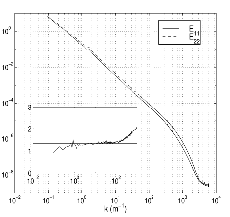
FIG. 1.: Longitudinal and transverse spectral densities, Taylor microscale Reynolds number $\approx 19,000$.

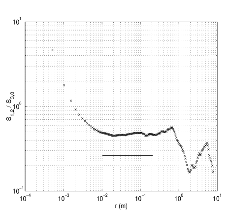
FIG. 2.: The ratio of $S_{1,2}$ to $S_{3,0}$ showing some deviations from the isotropic value of $1/3$ in the inertial range. In this figure and elsewhere, the horizontal bar in the figure represents a conservative extent of the scaling region determined from Kolmogorov’s 4/5-ths law.

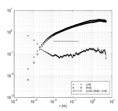
FIG. 3.: The terms of Eq. (16) with their relative difference.

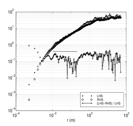
FIG. 4.: The terms of Eq. (17) with their relative difference.

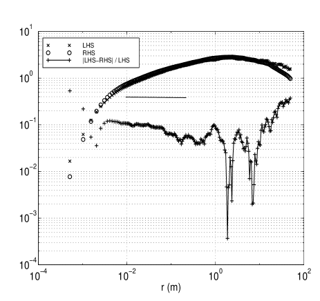
FIG. 5.: The terms of Eq. (18) with their relative difference.

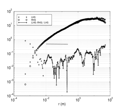
FIG. 6.: The terms of Eq. (19) with their relative difference.

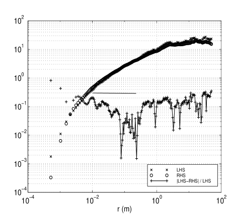
FIG. 7.: The terms of Eq. (20) with their relative difference.

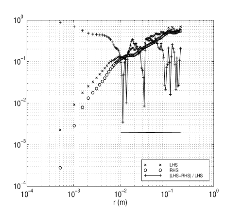
FIG. 8.: The terms of Eq. (21) with their relative difference.

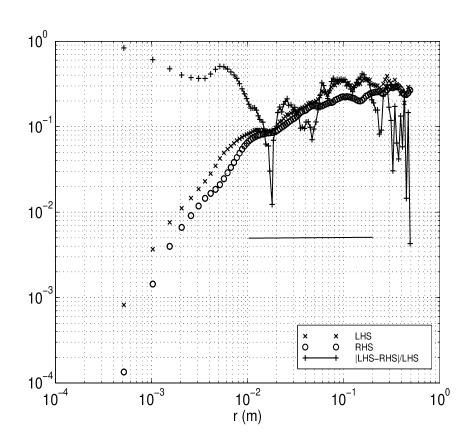
FIG. 9.: The terms of Eq. (22) with their relative difference.

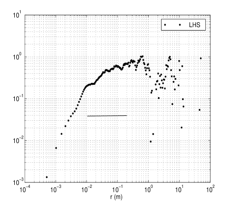
FIG. 10.: The terms of Eq. (23) with their relative difference.

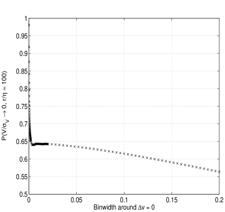
FIG. 11.: The value of the PDF as $V/\sigma_{V}\rightarrow 0$ for $r\approx 100\eta$ for different binwidths.

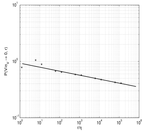
FIG. 12.: Log-log plot of the peak values of the PDFs of transverse velocity increments. The line indicates a slope of -0.065.

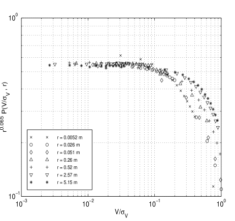
FIG. 13.: Log-log plot of the near-peak values of the PDFs of transverse velocity increments. The collapse of the data occurs for the normalization $r^{\kappa}P(V/r^{\kappa})$ where $\kappa=0.065$.

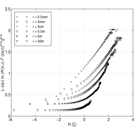
FIG. 14.: The tails of the PDFs in the form required by the theory (see Eq. (42). Lognormality of the tails requires that the data follow straight lines.

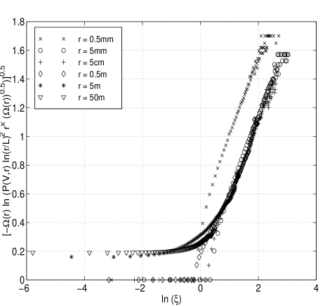
FIG. 15.: The collapsed tails of the PDF from the previous plot, taking into account an ad hoc prefactor of $(\ln(r/L))^{2}$.

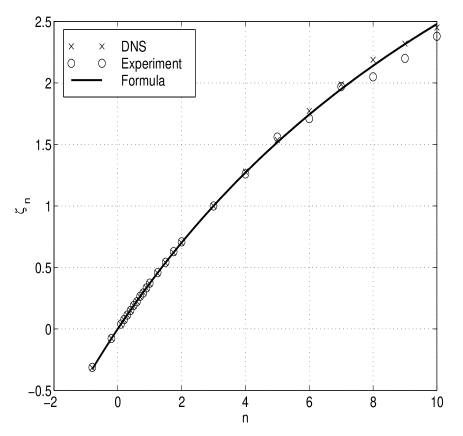
FIG. 16.: Comparison of the DNS and experimental values of $\zeta_{n}$ with those from Eq. (43). The numbers in the plot are for longitudinal structure functions, but these are identical to those for transverse structure functions in the isotropic sector see [8, 9].

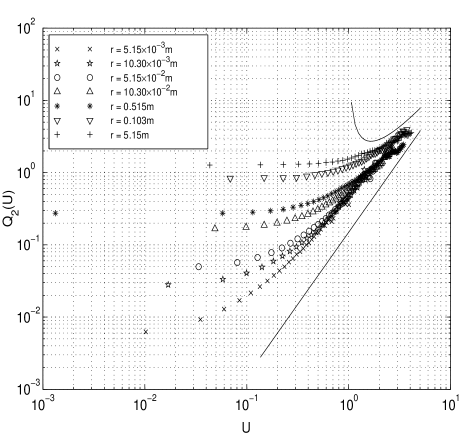
FIG. 17.: $Q_{2}(U)$, the conditional expectation value of $V^{2}$ on $U$ for various different $r$, on a log-log scale. The upper solid line indicates $U^{2}/log(U^{2})$, the lower solid line indicates the $U^{2}$ scaling slope.

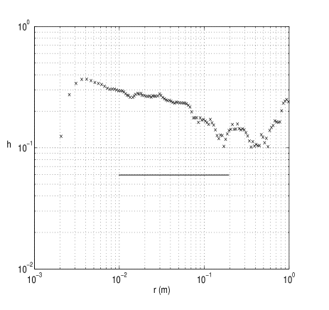
FIG. 18.: The coefficient $H$ of the pressure term computed by substituting Eq. (52) in Eq. (46) with $n=1$.

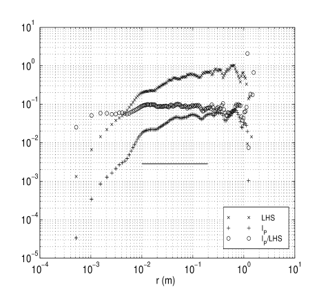
FIG. 19.: The LHS and pressure terms of Eq. (47) with $n=2$ and $H=0.25$ in the pressure model; the ratio indicates that the pressure term as computed from the model is about 10$\%$ of the balance.

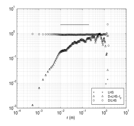
FIG. 20.: The terms of Eq. 47 with $n=2$, $H=0.25$; the difference LHS-RHS indicates the magnitude of the dissipation term.

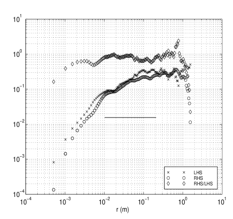
FIG. 21.: The LHS and RHS of the approximate equation, Eq. (22), without pressure or dissipation terms. The RHS balances the equation up to about 80$\%$ in the inertial range, less as we approach the dissipation and large scales.

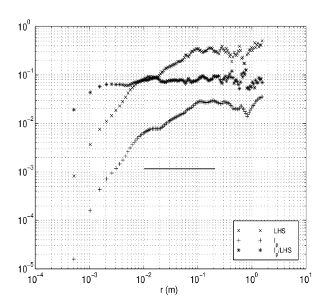
FIG. 22.: The LHS and pressure terms $I_{p}$ of Eq. (55) with their ratio showing that the pressure only accounts for about 8-10$\%$ of the balance, less as one approaches the dissipative scales and large scales.

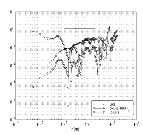
FIG. 23.: The LHS and dissipation terms $D$ of Eq. (55) with the dissipation computed by subtracting the RHS and the pressure (see Fig. 22) from LHS; the ratio of $D$ to LHS indicates a large scatter but shows the dissipation contributes in the inertial range only to about 10$\%$, but that it significantly increases towards the dissipative scales.

REFERENCES

- [1] A.N. Kolmogorov, Dokl. Akad. Nauk. SSSR. 32, 19 (1941).
- [2] V. Yakhot, Phys. Rev. E 63, 026307 (2001).
- [3] R.J. Hill, J. Fluid Mech. 434, 379 (2001).
- [4] A.N. Kolmogorov, J. Fluid Mech. 13, 82 (1962).
- [5] A.N. Kolmogorov, Dokl. Akad. Nauk. SSSR 30, 299 (1941).
- [6] B. Dhruva, Y. Tsuji and K.R. Sreenivasan, Phys. Rev. E 56, 4928 (1997).
- [7] B. Dhruva, An experimental study of high Reynolds number turbulence in the atmosphere. Ph.D. thesis, Yale University (2000).
- [8] I. Arad, B. Dhruva, S. Kurien, V.S. L’vov, I. Procaccia and K.R. Sreenivasan, Phys. Rev. Lett. 81, 5330 (1998).
- [9] S. Kurien and K.R. Sreenivasan, Les Houches Summer School Proceedings, Springer and EDP-Sciences, pp. 1-60, 2001.
- [10] A.S. Monin and A.M. Yaglom, Statistical Fluid Mechanics, Volume 2, MIT Press, 1975.
- [11] I. Arad, L. Biferale, I. Mazzitelli and I. Procaccia, Phys. Rev. Lett. 82, 5040 (1999).
- [12] A. Vincent and M. Meneguzzi, J. Fluid Mech. 225, 1 (1991).
- [13] J. Jimenez, A.A. Wray, P.G. Saffman and R.S. Rogallo, J. Fluid Mech. 225, 65 (1993).
- [14] X. Shen and Z. Warhaft, Phys. Fluids 11, 2976 (2000).
- [15] G. Boffetta, A. Celani and M. Vergassola, Phys. Rev. E 61, 29 (2000).
- [16] J. Paret and P. Tabeling, Phys. Rev. Lett. 79, 4162 (1997).
- [17] C. Meneveau and K.R. Sreenivasan, J. Fluid Mech. 224, 429 (1991).
- [18] A.M. Obukhov, J. Fluid Mech. 13, 77 (1962).
- [19] K.R. Sreenivasan, Rev. Mod. Phys. 71, S383 (1999).
- [20] G. Stolovitzky and K.R. Sreenivasan, Rev. Mod. Phys. 66, 229 (1994).
- [21] V. Yakhot and S.A. Orszag, J. Sci. Comp. 1, 3 (1986).
- [22] U. Frisch and J.-D. Fournier, Phys. Rev. A 17, 747 (1978).
- [23] S. Kurien, Anisotropy and the universal properties of turbulence. Ph.D. Thesis, Yale University (2001).
- [24] M. Jensen, P. Guliani and V. Yakhot (unpublished).
- [25] N. Cao, S. Chen and Z. She, Phys. Rev. Lett. 76, 3711 (1996).
- [26] T. Gotoh and D. Fukayama, Phys. Rev. Lett. 86, 3775 (2001).