A Simple Model of Epidemics with Pathogen Mutation

Abstract

We study how the interplay between the memory immune response and pathogen mutation affects epidemic dynamics in two related models. The first explicitly models pathogen mutation and individual memory immune responses, with contacted individuals becoming infected only if they are exposed to strains that are significantly different from other strains in their memory repertoire. The second model is a reduction of the first to a system of difference equations. In this case, individuals spend a fixed amount of time in a generalized immune class. In both models, we observe four fundamentally different types of behavior, depending on parameters: (1) pathogen extinction due to lack of contact between individuals, (2) endemic infection (3) periodic epidemic outbreaks, and (4) one or more outbreaks followed by extinction of the epidemic due to extremely low minima in the oscillations. We analyze both models to determine the location of each transition. Our main result is that pathogens in highly connected populations must mutate rapidly in order to remain viable.

]

I Introduction

The memory immune response enables humans and other animals to rapidly clear, or even prevent altogether, infection by pathogens with which they have previously been infected. For example, we typically contract chicken pox only once in our lifetime because of the effectiveness of the memory immune response, and vaccines are designed around the knowledge that our immune systems will more efficiently fight foreign invaders if already exposed to something very similar. Consequently, it is easy to imagine why some pathogens, such as influenza, use a strategy of disguise to survive in a host population. In most cases, this disguise is facilitated by mutation: pathogens permanently change their genetic content in order to alter their appearance to the host immune system. With enough mutations, a pathogen will ultimately be unrecognizable to the immune system of a host that has previously been infected with one of its ancestors. In this paper, we study the dynamics of populations that lose immunity via this route.

In epidemiological models, host populations are traditionally categorized into three states: susceptible to infection ($S$), infected ($I$), and removed or immune ($R$). The succesion of states we will study is depicted in the following diagram:

Models that describe such an epidemiological cycle are referred to as $SIRS$ models. While there is a vast literature covering models in which the “loss of immunity” step is not considered (referred to as $SIR$ models; see for example the classic texts by Bailey [1], Anderson and May [2] and the recent review by Hethcote [3]), comparatively little work has been done to understand how the nature of the $R\to S$ transition affects the dynamics of an epidemic.

In principle, the transition depends on the strain to which one is exposed (the challenge strain), in addition to one’s previous history of infection. We thus begin our analysis with a computational “bitstring model” in which different pathogen strains are represented by bitstrings that can mutate. In this model, immunity depends explicitly on the history of strains with which one has been infected. We find four fundamentally different types of behavior, depending on parameters: (1) pathogen extinction due to lack of contact between individuals, (2) endemic infection (steady state infection), (3) periodic epidemic outbreaks (sustained oscillations), and (4) one or more outbreaks followed by extinction of the epidemic due to extremely low minima in the oscillations (“dynamic extinction”).

We then develop a difference equation model in which the nature of immunity is significantly simplified. Instead of acquiring indefinite immunity to a specific pathogen, individuals in this reduced model spend a fixed number of time steps in a generalized immune class before being returned to the susceptible population. This $SIR_{1}R_{2}\cdots R_{N}S$ model has been studied extensively by Cooke et al. [4] and also by Longini [5], who used stochastic methods to investigate the model with immunity lasting only a single time step. The same four qualitatively different dynamics seen in the bitstring model are also observed for this model. We extend Cooke’s work by deriving the location of the onset of oscillatory dynamics in any dimension (which is determined by the number of time steps spent in the immune class). Stability is lost through a Hopf bifurcation, and changes in the model parameters can increase the resulting limit cycle amplitude to the point that the minimum becomes extremely small. We establish a criterion for “dynamic extinction” (for which the minimum fraction infected in the limit cycle oscillation is less than $1/N$, where $N$ is the population size) and construct an asymptotic approximation for the location of this extinction transition.

II Bitstring model

The immune response recognizes foreign molecules in a highly specific way. Individual immune cells or antibodies that recognize a protein from one pathogen strain may be unable to recognize a similar protein derived from another pathogen strain. Because protein sequence and structure is determined by the genetic content of an organism, immune responses to a pathogen are in fact specific to the pathogen’s genetic content. We thus introduce a bitstring model in which pathogen strains are represented by bitstrings, where the bitstring is regarded as an abstract representation of a pathogen’s genetic code. Hosts are immune to infection by pathogens that are highly similar to pathogens with which they have been previously infected, where similarity between two strains is measured by hamming distance [6].

The model consists of $N$ individuals who are either uninfected or infected with a strain represented by one of the $2^{\ell}$ possible bitstrings of fixed length $\ell$ [7]. Individuals keep a record of all the strains with which they have been infected, and we refer to these histories as their memory repertoire. Once per time step, each infected individual exposes $z$ others by selecting individuals uniformly at random from the entire population [8]. The susceptibility of a contacted individual is determined by comparing the bitstring of the challenge strain with the bitstrings of all strains in the memory repertoire. Specifically, an individual is susceptible if $h_{\min}>h_{\text{thr}}$, where $h_{\text{thr}}$ is a parameter, and $h_{\min}$ is the smallest hamming distance between the challenge strain and any strain in the individual’s memory repertoire. With probability $\mu$ the challenge strain mutates by flipping one randomly chosen bit; otherwise the strain remains unchanged. In each case considered here, we keep $\mu$ fixed at $0.1$ and vary the threshold hamming distance $h_{\text{thr}}$; these two parameters are inversely proportional. Infection lasts a single time step, and strain transmissibility is determined exclusively by individual immune responses, i.e., in an entirely susceptible population no strain is more fit than any other.

FIG. 1.: The dynamics of infection in the bitstring model. (a) Fraction of population infected versus time for two different threshold hamming distances. For the smaller value of $h_{\text{thr}}$, $p$ relaxes to a steady state value. At the larger value, the disease does not persist. (b) The hamming distance from the founder strain averaged over all strains present. (c) The standard deviation of the distance from the founder strain. This is a measure of the diversity of strains present.

In the first time step, one randomly chosen individual is infected with the bitstring $000\cdots 000$ and all others have never been infected. From this initial condition we observe three long term behaviors. The first is trivial: when $z<1$, the size of the epidemic goes to zero since on average each individual will expose fewer than one other individual. The remaining behaviors are (1) the fraction of the population that is infected, $p$, approaches either a steady state nonzero value or (2) after a brief outbreak, the epidemic dies out. Figure 1a shows the difference in these two types of behavior. Interestingly, the transition from persistence to extinction occurs as we increase $z$.

FIG. 2.: Boundary between pathogen persistence and extinction in the bitstring model. Results were obtained by averaging the greatest value of $h_{\text{thr}}$ at which the pathogen persisted over 150 runs, for each value of $z$.

For a more complete characterization of this route to pathogen extinction, we ran simulations at every integer–valued point in the $z$–$h_{\text{thr}}$ plane with $0<h_{\text{thr}}<10$ and $0<z<30$. Figure 2 shows the result: below the curve, the epidemic persists, and above the epidemic dies out. Interestingly, $h_{\text{thr}}$ is a decreasing function of $z$, meaning a high contact rate is actually detrimental to the pathogen’s ability to persist in a population. We can explain this result intuitively: the greater the value of $z$, the greater the average number of previous infections any given host will have. This implies that every individual will have a larger memory repertoire, and thus each strain’s ability to infect a host will be reduced.

Increasing $h_{\text{thr}}$ also causes extinction to occur. This happens because the number of strains to which an individual is immune increases with $h_{\text{thr}}$, and thus reduces the likelihood of infection. Increasing $h_{\text{thr}}$ can also be thought of as decreasing the pathogen mutation rate, since the memory immune response will be more effective if the pathogen changes less rapidly.

When persistence occurs, the fraction of the population infected is close to one (Figure 1a). This is in contrast to results from single strain $SIR$ models, which typically predict that the fraction of infected individuals is proportional to (and less than) $1-1/R_{0}$, where $R_{0}$ is the number of new infections that would result from a single infection in a completely susceptible population [2] – this is $z$ in our case. In Figure 1a, the fraction infected at equilibrium is approximately 0.99, certainly greater than $1-1/z=0.8$. This discrepancy occurs because there is more than one strain present in the bitstring model, and individuals can be infected by two different strains in two consecutive time steps. Figures 1b–c illustrate this effect: in the case when persistence occurs, the mean hamming distance from the founder increases steadily in time, and the diversity of strains present (measured by the standard deviation) is high. In contrast, when $z$ is increased and extinction occurs, one can see that although the diversity is initially higher, prior to extinction it is lower than in the persisting case.

FIG. 3.: Nucleotide substitutions in the nonstructural genes of influenza A. Figure reproduced with permision from Buonagurio et al. [9]

In the absence of immunity, no single strain has a competetive advantage over another in the bitstring model. However, there is evidence to suggest that in the case of influenza, there are selective pressures that constrain base pair subsititions to a small part of the entire genomic sequence space (i.e., with little diversity) and the number of substitutions increases linearly in time [9] (Fig. 3). This motivates us to consider a special form of the model where bitstring mutation goes only in one direction, e.g., 000…000 $\to$ 100…000 $\to$ 1100…000, etc. Specifically, when mutation occurs, rather than flipping a randomly chosen bit, the leftmost zero in the bitstring sequence is changed to a 1. All other model mechanisms are as before.

FIG. 4.: The dynamics of infection when bitstring evolution is constrained to go in one direction. We have used $h_{\text{thr}}=4$.

Figure 4 shows that under these assumptions, the system’s dynamics are quite different. Most notably, as the contact rate $z$ increases from $z=1.25$ to $z=2$, sustained oscillations emerge from what appears to be steady state behavior surrounded with stochastic noise. As these oscillations increase in amplitude, the minimum number of infected individuals ultimately gets so low that the epidemic dies out due to the population’s finite size (at $z=4$).

FIG. 5.: The dynamics of infection in the bitstring model with directed evolution. (a) Fraction of population infected versus time for two different threshold hamming distances. For the smaller value of $h_{\text{thr}}$, $p$ converges to oscillatory behavior. At the larger value, the disease does not persist; the minimum number of infected individuals gets too low. (b) The hamming distance from the founder strain averaged over all strains present. The distance increases linearly with time, in contrast to the results in Figure 1. (c) The standard deviation of the distance from the founder strain. This is a measure of the diversity of strains present.

Figure 5 depicts the dynamics in sequence space for the last two cases from Fig. 4. In contrast to Figure 1, the hamming distance from the founder strain increases linearly in time and the diversity is low. These results mirror what has been observed for influenza, and motivate us to understand the dynamics of this particular system in more detail.

Under the assumption that pathogen evolution is constrained to be linear in time, a further simplification of the system may be obtained by assuming that individuals are immune for a fixed period of time after infection. In the following sections, we analyze a difference equation model for this scenario to gain insight into the series of transitions observed in Figure 4.

III Immunity Model

A Model Derivation

In this section, we derive a system of difference equations to model the average behavior of a closed population of susceptible, infective, and immune individuals. Upon infection, individuals spend one time step in the infective class, and the subsequent $\tau-1$ time steps in the immune class. After these $\tau$ time steps, individuals are returned to the susceptible pool. The total population size is $N$ and there are no births or deaths (i.e., $N$ is constant).

We define $p_{t+1}$ as the probability that an individual is infected at time $t+1$:

$$p_{t+1}=x_{t}s_{t},$$ (1)

where $x_{t}$ is the probability that an individual is exposed at time $t$, and $s_{t}$ is the probability of residing in the susceptible class. At each time step, the $Np_{t}$ infected individuals make $z$ random exposures. The probability that an individual is not involved in any such encounter is simply $(1-1/N)^{Np_{t}z}$, and so the probability of exposure can be expressed as:

$$x_{t}=1-\left(1-\frac{1}{N}\right)^{Np_{t}z}.$$ (2)

The fraction of the population that is immune at any given time $t$, can be determined by examining the fraction which has been infected in any of the previous $\tau-1$ time steps, $\sum_{k=1}^{\tau-1}p_{t-k}$. The probability that an individual is susceptible is simply the probability of being neither infected nor immune:

$$s_{t}=1-\sum_{k=0}^{\tau-1}p_{t-k}.$$ (3)

This gives

$$p_{t+1}=\left(1-\left(1-\frac{1}{N}\right)^{Np_{t}z}\right)\left(1-\sum_{k=0}^{\tau-1}p_{t-k}\right),$$ (4)

which simplifies to

$$p_{t+1}=(1-e^{-zp_{t}})(1-\sum_{k=0}^{\tau-1}p_{t-k})$$ (5)

in the large system limit, $N\to\infty$. Thus, we have reduced the immunity model to a $\tau$ dimensional map, or equivalently a system of $\tau$ difference equations. For large populations, the equations are independent of $N$, and thus the only parameters are $\tau$ and $z$. This model was originally introduced by Cooke et al. [4].

B Dynamics

Numerical iteration of Eq. (5) from the initial conditions $p_{i}=0,i=1\dots\tau-1$ and $p_{\tau}=10^{-4}$ yields the same four types of long term behavior observed in the bitstring model: approach to the trivial equilibrium ($p_{t}\to 0$, not shown), approach to a nonzero equilibrium (Fig. 6a), sustained oscillations that are generally quasiperiodic (Fig. 6b–c), and dynamic extinction (Fig. 6d). Dynamic extinction occurs only due to numerical roundoff error, and is not an analytical feature of Eq. (5). As we increase $z$ or $\tau$, $p_{t}$ eventually becomes so small at the minimum of the oscillation that $(1-e^{-zp_{t}})$ in Eq. (5) numerically evaluates to zero. Furthermore, oscillations do not occur for $\tau\leq 2$.

FIG. 6.: Fraction of population infected versus time for $\tau$=6 and various values of $z$. (a) For $z=2$, $p_{t}$ relaxes to a fixed point. (b) For slightly larger values of $z$, $p_{t}$ exhibits small amplitude quasiperiodic oscillations. (c) At $z=11$, true period 15 behavior emerges. (d) For $z=13$, $p_{t}$ exhibits quasiperiodic oscillations that are heavily weighted by small values.

For a fixed $\tau$, we observe that $p_{t}$ relaxes to a fixed point for small enough $z$. When $z<1$, $p_{t}$ approaches the trivial zero solution. As $z$ is increased through $z=1$, the non-zero equilibrium becomes an attractor. At some larger value of $z$, the fixed point loses stability and small amplitude quasiperiodic oscillations appear symmetrically centered around the former equilibrium point. As $z$ is further increased, the oscillations grow in amplitude and the system spends a large fraction of its time with only a small portion of individuals infected. Careful examination of the oscillations in this regime suggest they consist of two phases: exponential growth followed by rapid decay (Fig. 7).

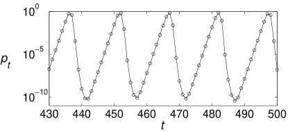
FIG. 7.: Fraction of population infected versus time for $\tau=6$ and $z=13$, plotted on a semilog scale. The data set used in the above plot is the same as the one used in figure 6d.

For certain combinations of $\tau$ and $z$, the oscillations are truly periodic rather than quasiperiodic. We observe few patterns in the location of these periodic solutions in the parameter space. However, we note that in the somewhat rare cases in which periodic behavior emerges, the period is generally longer for larger values of $z$ and $\tau$.

In the following sections we use linear stability analysis to determine the location of the transitions from the trivial equilibrium to the nonzero steady state and from the nonzero steady state to oscillations. The transition to dynamic extinction is determined by deriving an approximate expression for the minimum value of the oscillation and postulating that extinction occurs when this value goes below $1/N$ where $N$ is any desired population size. Figure 8 illustrates the location of these transitions in the $z-\tau$ plane.

FIG. 8.: The boundary between persistence and extinction for different population sizes. For each value of $\tau$, $z$ was increased until the minimum expected fraction of infected individuals declined below $1/N$, for $N=10^{5},10^{10}$, and $10^{15}$. The epidemic is considered extinct in the upper right region of the figure because the minimum of the oscillation is below $1/N$.

C Stability Analysis

The fixed points of the system satisfy

$$p^{\star}=(1-e^{-zp^{\star}})(1-\tau p^{\star}).$$ (6)

Making the substition $q_{t}=p_{t}-p^{\star}$ and linearizing about $p^{\star}$, we obtain

$$q_{t+1} = \Big{(}ze^{-zp^{\star}}(1-\tau p^{\star})+e^{-zp^{\star}}-1\Big{)}q_{t}$$ (8)

$$+\Big{(}e^{-zp^{\star}}-1\Big{)}\sum_{k=0}^{\tau-1}q_{t-k}.$$

Introducing the eigensolution $q_{t}=q_{o}\lambda^{t}$ yields a polynomial for the roots $\lambda_{i}$:

$$\lambda^{\tau}+\alpha\lambda^{\tau-1}+\beta\lambda^{\tau-2}+...+\beta\lambda+\beta=0,$$ (9)

where $\alpha=1-e^{-zp^{\star}}(1+z-z\tau p^{\star})$, and $\beta=1-e^{-zp^{\star}}$.

When the $\tau$ roots to this equation all lie within the unit circle in the complex plane, the fixed point in question will be stable.

Case i. $p^{\star}=0$. The first solution to Eq. (6) is

$$p^{\star}=0.$$ (10)

At this point, the eigenvalue equation simplifies to

$$\lambda^{\tau}-z\lambda^{\tau-1}=0.$$ (11)

The first $\tau-1$ roots of this equation are $\lambda=0$. The final solution solves $\lambda-z=0$, and thus the only eigenvalue of interest for stability is

$$\lambda=z,$$ (12)

indicating that the trivial equilbrium is stable for all $z<1$. Not surprisingly, this agrees with our previous results from the bitstring model in Section II, since if $z<1$, fewer than one new infection will result from each currently infected individual.

Case ii. $p^{\star}\neq 0$. The results in Figure 6 suggest that when $z>1$, the nonzero solution to Eq. (6) becomes stable. Indeed, Cooke et al. have shown for all $z>1$ that this point is globally stable when $\tau=1$, and locally stable when $\tau=2$. They conjectured that when $\tau=3$, the fixed point loses stability at $z=4.58$. Here we will verify this result and obtain the transition for all $\tau\geq 3$ by finding the location of the bifurcation at which the quasiperiodic orbits emerge.

As before, the onset of instability occurs when $|\lambda_{i}|=1$ for one or more $\lambda_{i}$. Therefore, to locate the transition, we substitute $\lambda=e^{i\phi}$ into Eq. (9). This yields two new equations, one for the real part and one for the imaginary part:

$$1-e^{-zp^{\star}}-(1-\tau p^{\star})ze^{-zp^{\star}}=\frac{\cos(\phi)-\cos(\phi(\tau+1))}{\cos(\tau\phi)-1}$$ (13)

$$1-e^{-zp^{\star}}=\frac{2\sin(\phi)-\sin(2\phi)}{\sin(\phi(\tau-1))+\sin(\phi)-\sin(\tau\phi)}$$ (14)

Combining these two equations with the expression for $p^{\star}$ (Eq. (6)), we have three equations for four unknowns ($p^{\star},\tau,z,$ and $\phi$). These three equations define the Hopf curve.

FIG. 9.: Hopf curve generated by numerically solving equations (6) and (13) simultaneously for specified values of $\tau$. The open circle marks the location of the transition previously derived by Cooke et al. [4]. The solid line is our asymptotic solution, taken to $O(1/\tau^{3})$.

Figure 9 shows the numerically generated solution for the Hopf curve in the $z$–$\tau$ plane. The dependence on parameters is clearly similar to what we observed in the biststring model as that system switched from persistence to extinction. For $z<1$, $p^{\star}=0$ is the only attractor. When $z>1$ below the Hopf curve, the stable fixed point is given by the non–zero solution to Eq. (6).

For large $\tau$, we can write a perturbative solution for the Hopf curve. Defining a new variable $\epsilon=\frac{1}{\tau}$, we can express $\phi,z,$ and $p^{\star}$ as power series in $\epsilon$:

$$z = 1+\sum_{i=1}^{\infty}a_{i}\epsilon^{i},$$ (15)

$$p^{\star} = \sum_{i=2}^{\infty}b_{i}\epsilon^{i},$$ (16)

$$\phi = \sum_{i=1}^{\infty}c_{i}\epsilon^{i}.$$ (17)

Solving perturbatively for the $a_{i}$, $b_{i}$, and $c_{i}$ gives

$$z = 1+\frac{\pi^{2}}{2}\epsilon+\frac{3\pi^{2}}{4}\epsilon^{2}+\frac{5}{96}(12\pi^{2}+\pi^{4})\epsilon^{3}+O(\epsilon^{4}),$$ (18)

$$p^{\star} = \frac{\pi^{2}}{2}\epsilon^{2}+\frac{1}{4}\pi^{2}(2-\pi^{2})\epsilon^{3}+O(\epsilon^{4}),$$ (19)

$$\phi = \pi\epsilon+\frac{\pi}{2}\epsilon^{2}+\frac{\pi}{4}\epsilon^{3}+O(\epsilon^{4}).$$ (20)

Figure 9 shows that for large $\tau$, the perturbative solution for the bifurcation curve agrees well with the numerical solution.

The variable $\phi$ may be thought of as the rotation number [10] of the solution to the linearized equations. In cases where a periodic orbit emerges at the bifurcation, $2\pi/\phi$ will be the period of the orbit, and in cases where the orbit is quasiperiodic, the approximate pattern will repeat itself on average every $2\pi/\phi$ time steps.

Eq. (20) indicates that $\phi$ is a decreasing function of $\tau=1/\epsilon$, meaning that the period of the epidemic oscillations will increase with $\tau$. In other words, we expect oscillations to occur less frequently as the duration of immunity increases.

D Relaxation Oscillations and the Route to Extinction

As pointed out earlier, Figure 7 suggests that as $z$ and $\tau$ become large, the system’s dynamics can be characterized by exponential growth followed by rapid decay, with short transitional phases between the two regimes. In this section, we explore the relaxation oscillations by deriving equations that approximate the system’s behavior in the various phases.

We begin by focusing on a single oscillation as pictured in Figure 10. As $p_{t}$ grows exponentially toward its maximum, the fraction of individuals infected at the current time and the previous $\tau-1$ time steps is small enough that, to a first order approximation, Eq. (6) can be rewritten as

$$p_{t+1}\approx zp_{t}\qquad\textrm{(in the growth phase)}.$$ (21)

The behavior persists until $zp_{t}$ reaches order 1. We make the assumption that Eq. (21) holds until the point $p_{0}$ and check for consistency after subsequent calculations. For times less than $t=0$, we can write $p_{-t}=p_{0}/z^{t}$.

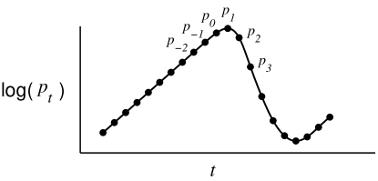
FIG. 10.: Generic form of a relaxation oscillation for large $z$ and $\tau$. The oscillation is characterized by exponential growth followed by rapid decay.

Next, we iterate the $\tau$–dimensional map using the unkown form of $p_{0}$ to find $\tilde{p}_{\min}(p_{0})$. The tilde notation indicates that $\tilde{p}_{\min}$ is a local minimum of the oscillations. To find the global minimum, we must find the value of $p_{0}$ that minimizes $\tilde{p}_{\min}$. In what follows, we derive an approximation for $p_{\min}$ in the large $z$ limit. This calculation requires that the points near the transition phase be handled individually before a general expression for the decay behavior may be obtained. We determine $p_{1}$, $p_{2}$, and $p_{3}$ explicitly and then derive the general form for $p_{t+1}$ for $t\geq 3$.

A reasonable approximation for $p_{1}=x_{0}s_{0}$ is obtained by including only the first term that appears in the sum in $s_{0}$:

$$p_{1}\approx\left(1-\exp(-zp_{0})\right)(1-p_{0})$$ (22)

Next, $p_{2}$ can be determined by first considering the probability of exposure at time $t=1$. Since the fraction of individuals infected is order one at the maximum point of the oscillation, the probability of exposure at time $t=1$ goes to one in the limit of large $z$. This implies that virtually all individuals who are susceptible at time $t=1$ will become infected at time $t=2$: $p_{2}\approx s_{1}$.

In order to produce a simple expression for $p_{2}$, it useful to note that the fraction of individuals which reside in the susceptible class at any point in time can be written in terms of the same fraction at the previous time step:

$$s_{t} = \exp(-zp_{t-1})s_{t-1}+p_{t-\tau}.$$ (23)

Using this, we write $p_{2}$ in a convenient form:

$$p_{2}\approx s_{1}\approx\exp(-zp_{0})(1-p_{0})+\frac{p_{0}}{z^{\tau-1}}.$$ (24)

To find $p_{3}$, the final point in the transition region, we note that $s_{2}\approx p_{2-\tau}\approx\frac{p_{0}}{z^{\tau-2}}$, since $zp_{1}\gg 1$. Assuming $zp_{2}$ is small, we obtain:

$$p_{3}\approx zp_{2}s_{2}=\frac{p_{0}}{z^{\tau-3}}p_{2}.$$ (25)

The general behavior in the decay regime can be derived by examining the fraction of individuals susceptible for $3\leq t\leq\tau$. In this region, $s_{t-1}$ is small compared to $p_{t-\tau}$, yielding:

$$s_{t} \approx p_{t-\tau}\approx\frac{p_{0}}{z^{\tau-t}}\qquad\textrm{(for $3<t<\tau$)}.$$ (26)

Since $zp_{t}$ is small in the decay phase, the probability of exposure depends linearly on the fraction of individuals infected: $x_{t}\approx zp_{t}$. Thus, we see that for $t\geq 3$, we can again replace the original set of $\tau$ difference equations by a single equation:

$$p_{t+1}=z^{t-\tau+1}p_{0}p_{t}.\qquad\textrm{(for $3<t<\tau$)}.$$ (27)

The minimum of $p_{t}$ occurs when $z^{t-\tau+1}p_{0}$ becomes greater than 1. If we assume that $p_{0}$ lies between $\frac{1}{z}$ and 1, as is consistent with our earlier assumption that Eq. (21) holds until $t=0$, then the minimum must occur at $t=\tau$. Consequently, we can express $p_{t}$ in terms of $p_{3}$ for times greater than $t=3$. Combining Eqs. (27) and (24), we obtain:

$$p_{\tau} = z^{-\frac{1}{2}(\tau^{2}-5\tau+6)}p_{0}^{\tau-2}p_{2}$$ (28)

Finding the minimum value of $p_{\tau}$ requires solving for the roots of the equation ${\rm d}p_{\tau}/{\rm d}p_{0}=0$, which yields

$$(\tau-2)\left(\frac{p_{0}\exp(zp_{0})}{z^{\tau-1}}+1-p_{0}\right)$$ (29)

$$+p\left(\frac{\exp(zp_{0})}{z^{\tau-1}}-1-z(1-p_{0})\right) = 0$$ (30)

We try a solution of the form

$$p_{0}=\frac{\log(f)}{z}.$$ (31)

Substituting this into Eq. (30) we obtain an asymptotic expression for $f$, which is valid to leading order as $z\to\infty$: $f\approx z^{\tau}/(\tau-1)$. This gives:

$$p_{0} \approx \frac{\tau\log(z)}{z},$$ (32)

which is consistent with our assumption that $p_{0}$ must lie between $1/z$ and 1.

Finally, to obtain $p_{\min}$, we insert (32) into our expressions for $p_{2}$ and $p_{\tau}$ (Eqs. (24) and (28)):

$$p_{\min}=z^{-\frac{1}{2}(\tau^{2}-\tau+2)}\left(\tau\log(z)\right)^{\tau-1}.$$ (33)

In the derivation of the difference equations in Section III A, we assumed an infinite population size. Under this assumption, the fraction of immune individuals can be arbitrarily close to 1 without driving the disease to extinction. If, however, we assume the population size is finite, at some point the minimum value of $p_{t}$ will be less than the fraction of the population equivalent to one individual, that is $p_{\min}<1/N$. Replacing $p_{\min}$ by $1/N$, we have an equation for the curve that separates the region of disease persistence from the region of extinction:

$$\frac{1}{N}=z^{-\frac{1}{2}(\tau^{2}-\tau+2)}\left(\tau\log(z)\right)^{\tau-1}.$$ (34)

Figure (11) compares the predictions of (34) with the data obtained from the map dynamics. We see that our predictions work quite well for large $z$. Note that the asymptotic approximation only fits the numerical data for unrealistically large population sizes (for smaller population sizes the extinction boundary occurs at smaller $z$). This is not too troublesome, however, since our overly-simplified model cannot be expected to quantitatively match actual population features. Rather, the strength of this approach is that it provides a clear picture of a mechanism for dynamic extinction.

FIG. 11.: Extinction curves for various values of system size $N$. The solid lines represent the asymptotic approximation for large $z$. Here, $N$ is merely a parameter that determines the condition of extinction for the difference equation model; it is not the number of nodes in a simulation as in the bitstring model. The disease is considered extinct if the fraction infected ever falls below $1/N$.

IV Conclusions

We have shown that oscillations in the number of infected individuals in a population could be due to a mutating pathogen. In both of the models we have studied, oscillations occur as a consequence of the continual introduction of novel strains, rather than the interplay between several pre–existing strain types (for studies of the latter, see references [11] and [12]). We can explain this phenomenon naturally in terms of single outbreak epidemics: each period of oscillation can be regarded as a new epidemic with a new strain to which few if any individuals have immunity.

In the $\tau$–dimensional map, oscillations occur only for an intermediate range of immunity duration $\tau$. If it is too short (or, equivalently, if the mutation rate is too high), oscillations do not occur because a significant pool of susceptible individuals is always present. Alternatively, if the duration of immunity is too long, the infected pool oscillates with increasingly large amplitude and ultimately becomes too small at its minimum for the pathogen to persist.

The presence of oscillations depends on the contact rate in a similar fashion. For low contact rates, the susceptible pool remains large and oscillations do not occur. For high contact rates, large amplitude oscillations force the number of infected individuals to such a small value that the epidemic dies out.

We have quantified the effect of contact rate and immunity duration on oscillatory behavior through Hopf bifurcation analysis to locate the onset of oscillations, and with asymptotic methods to determine their minimum value. In both analyses, the boundary between two types of behavior is marked by an inverse relationship between immunity duration and contact rate. In particular, in a population with high contact rates, pathogen persistence requires short periods of immunity (or high mutation rates) suggesting that highly connected population structure could provide selective pressure for rapidly mutating pathogens. This could lead to diseases that are more difficult to actively counteract through immunization programs.

There are two assumptions that could have significant impact on our results. First, these models operate in discrete time, where oscillations and chaotic dynamics are known to occur more readily. Second, we have assumed the underlying networks are fully mixed, but some sort of quasi-static network structure may be much more realistic. The addition of spatial effects could dampen oscillations, if two regions oscillated out of phase and thereby prevent global extinction of the pathogen.

Research supported in part by the National Science Foundation, Electric Power Research Institute, and Department of Defense. We thank Ken Cooke and Carlos Castillo-Chavez for helpful and interesting discussions.

REFERENCES

- [1] N. T. Bailey, The Mathematical Theory of Infectious Diseases, 2nd edition, London: Griffin (1975).
- [2] R. M. Anderson and R. M. May, Infectious Diseases of Humans, Oxford University Press, London (1991).
- [3] H. W. Hethcote, SIAM Review 42, 599–653 (2000).
- [4] K. L. Cooke, D. F. Calef, and E. V. Level, Nonlinear Systems and its Applications, Academic Press, New York 73–93 (1977).
- [5] I. M. Longini, Mathematical Biosciences 50, 85-93 (1980).
- [6] Hamming distance between two bitstrings is simply the number of bits that differ between them. For example, the hamming distance between and is .
- [7] Because simulations are carried out on a 32 bit computer, for simplicity . Changing this number would change the size of the “sequence space” through which the strains could move, but would not otherwise qualitatively change our results.
- [8] If is not an integer, infectives randomly expose either or individuals with weighted probability such that the average number of exposures is ; the model could easily be extended to other distributions.
- [9] D. A. Buonagurio, S. Nakada, J. D. Parvin, M. Krystal, P. Palese, and W. M. Fitch, Science 232, 980–982 (1986).
- [10] J. Guckenheimer and P. Holmes: Nonlinear Oscillations, Dynamical Systems, and Bifurcations of Vector Fields (Springer, 1983).
- [11] J. Lin, V. Andreasen and S. A. Levin, Mathematical Biosciences 162 33–51 (2000).
- [12] S. Gupta, N. Ferguson, R. Anderson: Science 280, 912 (1998).