[

Dynamics of a Tube Conveying Fluid

Abstract

A tube conveying a large amount of fluid with a free outlet does not sit still. We construct and analyze a nonlinear evolution equation describing such phenomena. Two types of boundary conditions at the inlet are considered, one for which it is clamped and one for which it is hinged. Analyzing the linear stability of the trivial solution, we find that with the former boundary conditions, it exhibits a “flutter” instability, while with the latter boundary conditions, it exhibits a “rotation” instability. These instabilities and the nonlinear behaviors of the system are also studied numerically.

]

Thready structures appear in a wide variety of physical systems and exhibit many different distinctive patterns and types of motion. For example, the behavior of chain polymers is a commonly studied topic in physics and chemistry. In fluid physics, the structures and dynamics of vortex filaments have been studied in detail. Biological systems provide us with many phenomena involving thready objects from microscopic to macroscopic scales, e.g., the behavior of DNA, the folding of proteins, the beating of flagellum, and the locomotion of snakes. These phenomena are observed in non-equilibrium systems in which several factors, such as elasticity, driving forces and dissipation, are balanced. In this class of phenomena, the motion of a tube conveying fluid with a free outlet has been extensively studied, owing to its simple nature. Paidoussis theoretically showed that the trivial, straight state becomes unstable at some flow rate, and the tube begins to flutter as the result of a Hopf bifurcation [2]. This result has been confirmed by several theoretical and experimental studies [3, 4, 5, 6, 7]. The theoretical models used in these studies are physically very realistic, but they are applicable only for small amplitude motion. Also, in most studies, only one type of boundary conditions (BC) is considered, that of the cantilevered type, in which the tube is clamped at the inlet and free at the outlet. In this Letter, we adopt a rather phenomenological approach to construct the minimal model for motion of any size amplitude under more general BC at the inlet. We obtain an evolution law in the form of a nonlinear integro-differential equation. A linear stability analysis of the trivial solution suggests not only the existence of a “flutter” instability but also the existence of a “rotation” instability, depending on the BC at the inlet. Numerical simulations confirm the existence of these instabilities and elucidate the nonlinear behavior of the equation.

We begin by deriving the evolution equations of the system. For this purpose, we first clearly define the physical system under consideration. Consider a tube conveying fluid with a free outlet. The motion is restricted to $x$-$y$ plane, and the gravitational force is not considered. Also, the length of the tube is regarded as fixed. We treat the tube as one-dimensional structure and ignore any dependence on its radius. An elastic force acts on the tube in response to its being bent from a straight shape. In the tube, fluid flows at a constant rate, and its momentum change creates a force acting transversely on the tube. A resistive force representing some kind of frictional interaction with a surrounding medium is also included. As typical cases, we consider two types of BC at the inlet. One case is that in which there is a clamp at the inlet, keeping both the position and direction fixed. The other is that in which there is a hinge at the inlet, keeping only the position fixed.

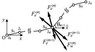
FIG. 1.: A discrete model of a tube. J_n and S_n denote the $n$th joint and segment, respectively. The $F_{e}^{(n-1)}$, two $F_{e}^{(n)}$, and $F_{e}^{(n+1)}$, all of the elastic forces that exert on J_n, act perpendicularly to the segments, and tend to straighten the tube. $F_{w}^{(n)}$, the force resulting from fluid flow, divides the angle $\angle$J_n-1J_nJ_n+1 in half, and tends to increase the bending.

We assume that a tube with the properties described above can be obtained as the continuum limit of the discrete articulated model depicted in Fig.1. In this model, there are $N+1$ joints and $N$ segments. Let $(x_{n},y_{n})$ be the coordinates of the $n$th joint, and let $\theta_{n}$ be the angle between the $n$th segment and the $x$ axis. Each joint has mass $m(N)\equiv M/N$, where $M$ is the total mass of the tube, and the segments have no mass. The fixed length of each segment is $l(N)\equiv L/N$, where $L$ is the total length of the tube. Each joint exerts an elastic force on itself and its neighboring joints that tends to straighten the tube. The magnitude of the force exerted is proportional to the difference between the angles of the segments on both sides: $F_{e}^{(n)}=k(N)\cdot|\theta_{n+1}-\theta_{n}|$ for $1\leq n\leq N-1$, where $k(N)$ is a positive coefficient representing the stiffness of the tube. The momentum change of the fluid flow at a joint creates a transverse force, which acts to increase the bending. The magnitude of this flow force is also proportional to the difference between the angles on both sides: $F_{w}^{(n)}=w(N)\cdot|\theta_{n+1}-\theta_{n}|$ for $1\leq n\leq N-1$ where $w(N)$ is a positive coefficient representing the flow rate. Here, we assume that $|\theta_{n+1}-\theta_{n}|\ll 1$. The directions and the joints on which the forces $\{\mbox{\boldmath$F$}_{e}^{(n)}\}$ and $\{\mbox{\boldmath$F$}_{w}^{(n)}\}$ act are exhibited in Fig.1. In addition to the above described forces, resistive forces act on each joint in the form ${\mbox{\boldmath$F$}_{v}^{(n)}}=-c(N)\cdot\mbox{\boldmath$v$}_{n}$ for $1\leq n\leq N$, where $\mbox{\boldmath$v$}_{n}$ is the velocity of $n$th joint and $c(N)$ is a positive coefficient representing the strength of the resistance. Since each segment has a fixed length, there are $N$ constraints. We account for these constraints by using Lagrange multipliers. As mentioned above, the inlet is either clamped or hinged. These conditions are realized by setting $F_{e}^{(0)}=k\theta_{1}$ if it is clamped and $F_{e}^{(0)}=0$ if hinged, where $F_{e}^{(0)}$ is a force that acts only on the first joint J₁.

Our next step is to derive evolution equations for this discrete model. To simplify the notation, we first restrict ourselves to the case of a clamped tube ($F_{e}^{(0)}=k\theta_{1}$). It is easy to write down $2N$ Newton’s equations of motion containing $N$ undetermined multipliers. The positions $\{x_{n},y_{n}\}$ can be rewritten in terms of the angles $\{\theta_{n}\}$ using the relation $(x_{n},y_{n})=l\sum_{i=1}^{n}(\cos{\theta_{i}},\sin{\theta_{i}})$. Eliminating the $N$ multipliers from these equations yields $N$ independent evolution equations for the generalized coordinates $\{\theta_{n}\}$. Assuming that inertial terms, such as those containing $\ddot{\theta}_{i}$, $\dot{\theta}_{i}^{2}$, are negligible (Physically, this is justified for a strongly dissipative system.), we obtain the rather simple equation

$$C\sum_{j=1}^{N}{\cal F}_{ij}\dot{\theta}_{j}=\sum_{j=1}^{N}A\cdot{\cal G}_{ij}\theta_{j}-B\cdot{\cal H}_{ij}(\theta_{j}-\theta_{j-1}).$$ (1)

Here, $A\equiv k/(ml)$, $B\equiv w/(ml)$, $C\equiv c/m$, $\theta_{0}\equiv 0$, and ${\cal F}_{ij}$, ${\cal G}_{ij}$ and ${\cal H}_{ij}$ are the components of $N\times N$ matrices defined as ${\cal F}_{ij}={\cal F}_{ji}\equiv(N-j+1)\cos(\theta_{i}-\theta_{j})$ for $j\geq i$, ${\cal G}_{ij}={\cal G}_{ji}\equiv(-2+\delta_{iN})\delta_{ij}+\delta_{i,j+1}$ for $j\geq i$, ${\cal H}_{ij}\equiv\cos{\{(\theta_{j}+\theta_{j-1}-2\theta_{i})/2\}}$ for $j>i$, ${\cal H}_{ij}\equiv 0$ for $j\leq i$.

The final step in constructing our model is to take the continuum limit $N\to\infty$ of (1). In this limit, the discrete index $n$ can be regarded as a continuous variable $s\in[0,L]$. Carrying out an integration by parts of the equation so obtained, we can write the evolution equation for the continuous model as

$$\int_{s}^{L}{\rm d}s^{\prime}\int_{0}^{s^{\prime}}{\rm d}s^{\prime\prime}\left\{\gamma\partial_{t}\theta(s^{\prime\prime})\right\}\cos{\{\theta(s)-\theta(s^{\prime\prime})\}}$$ (2)

$$= \alpha\partial_{s}^{2}\theta+\beta\sin{\{\theta(s)-\theta(L)\}},$$ (3)

with two BC:

$$\theta(0)=\partial_{s}\theta(L)=0.$$ (4)

Here, $\alpha\equiv\lim_{N\to\infty}[l^{4}A(N)]\mbox{, }\beta\equiv\lim_{N\to\infty}[l^{2}B(N)]$ and $\gamma\equiv\lim_{N\to\infty}C(N)$. These are constants independent of $N$. The convergence of these three limits is assumed, so that the three terms corresponding to the elasticity, the driving force resulting from fluid flow, and the dissipation are balanced.

In the case of a hinged tube ($F_{e}^{(0)}=0$), the evolution equation is derived in the very same way, although the result differs slightly from that of a clamped tube. For the discrete model, in this case the above definition of ${\cal G}_{ij}$ is replaced with ${\cal G}_{ij}={\cal G}_{ji}\equiv(-2+\delta_{iN}+\delta_{i1})\delta_{ij}+\delta_{i,j+1}$ for $j\geq i$. Then, for the continuous model, the two BC are not those given by (4), but rather,

$$\partial_{s}\theta(0)=\partial_{s}\theta(L)=0.$$ (5)

We see below that this slight difference has a great influence on the behavior of the whole system.

Note that we can always set $\gamma/\alpha=1$ and $L=1$ in (2) through rescaling of $t$ and $s$. This means that the number of essential parameters governing the behavior of the non-inertial tube is only one, say, $\beta/\alpha\equiv\epsilon>0$. Note that an increase of the flow rate corresponds to an increase of $\epsilon$. This rescaling leaves (2) as

$$\int_{s}^{1}{\rm d}s^{\prime}\int_{0}^{s^{\prime}}{\rm d}s^{\prime\prime}\left\{\partial_{t}\theta(s^{\prime\prime})\right\}\cos{\{\theta(s)-\theta(s^{\prime\prime})\}}$$ (6)

$$= \partial_{s}^{2}\theta+\epsilon\sin{\{\theta(s)-\theta(1)\}}.$$ (7)

We have thus derived the evolution equations for a clamped tube as (6) with (4) and for a hinged tube as (6) with (5). In each case we set $L=1$. Both systems have the same, trivial solution, $\theta(s)=0$, which corresponds to a completely straight tube. We now investigate situations in which this trivial solution becomes unstable by considering the linearization of (6) about this solution.

We first consider the case of a clamped tube. Assuming that for all $s\in[0,1]$, $|\theta(s)-0|\ll 1$ holds, we omit all but linear order terms in (6) to obtain

$$\int_{s}^{1}{\rm d}s^{\prime}\int_{0}^{s^{\prime}}{\rm d}s^{\prime\prime}\partial_{t}\theta(s^{\prime\prime})=\partial_{s}^{2}\theta+\epsilon\{\theta(s)-\theta(1)\}.$$ (8)

Unlike the nonlinear equation (6), the integrand depends only on $s^{\prime\prime}$. Thus, we can eliminate the integrals by differentiating (8) twice. Here, in order to retain all the information contained in (8), two conditions must be added to the differential equation that results from this procedure: Representing (8) as $F(s)\equiv[(\mbox{l.h.s.}-\mbox{r.h.s.})\mbox{ of (\ref{intlinear})}]=0$, this equation is equivalent to the differential equation $\partial_{s}^{2}F(s)=0$, together with the conditions $\partial_{s}F(0)=F(1)=0.$ We thus find that (8) is equivalent to

$$\partial_{t}\theta=-\partial_{s}^{4}\theta-\epsilon\partial_{s}^{2}\theta,$$ (9)

with the two extra BC

$$\partial_{s}^{3}\theta(0)+\epsilon\partial_{s}\theta(0)=\partial_{s}^{2}\theta(1)=0.$$ (10)

Now, our objective is to examine the eigenfunctions of (9) with the four BC given in (4) and (10). Expecting the existence of complex eigenvalues, we regard $\theta(s,t)$ as a complex variable $\Theta(s,t)\in\mbox{\boldmath$C$}$. Here, the linearized equation we consider is $\partial_{t}\Theta=-\partial_{s}^{4}\Theta-\epsilon\partial_{s}^{2}\Theta,$ with the four BC $\Theta(0)=\partial_{s}^{3}\Theta(0)+\epsilon\partial_{s}\Theta(0)=\partial_{s}\Theta(1)=\partial_{s}^{2}\Theta(1)=0$. Assuming the form $\Theta(s,t)\equiv e^{(\sigma+i\omega)t}\Phi(s)$, with $\sigma,\omega\in\mbox{\boldmath$R$}$, $\Phi\in\mbox{\boldmath$C$}$, we get

$$\qquad\qquad\quad-\Phi^{\prime\prime\prime\prime}-\epsilon\Phi^{\prime\prime}=(\sigma+i\omega)\Phi,$$ (11)

$$\quad\Phi(0)=\Phi^{\prime\prime\prime}(0)+\epsilon\Phi^{\prime}(0)=0\quad\;\;\;\mbox{clamped inlet,}$$ (12)

$$\quad\Phi^{\prime}(1)=\Phi^{\prime\prime}(1)=0\quad\qquad\qquad\;\>\,\mbox{free outlet.}$$ (13)

For a given $\epsilon$, the set of all such solutions $\{(\sigma,\omega,\Phi(s))\}$ may span the solution space of (11) with BC given in (12) and (13). However, all we want to know at present is when and how the trivial solution becomes unstable. For this reason, we set $\sigma=0$ in (11) to obtain

$$-\Phi^{\prime\prime\prime\prime}-\epsilon\Phi^{\prime\prime}=i\omega\Phi.$$ (14)

We now proceed to examine the solution set of (14), with the BC given in (12) and (13). First, we assume that the trivial solution becomes unstable beyond some critical value $\epsilon_{cr}$. Then, there necessarily exists at least one solution, $(\epsilon_{cr},\omega_{cr},\Phi_{cr})$. Note that this $(\epsilon_{cr},\omega_{cr},\Phi_{cr})$ need not be the critical mode itself when the $\sigma=0$ eigenspace is non-simple. In fact, such case exists for the hinged system.

The general solution of (14) is easily obtained. The characteristic polynomial of this equation is $L(P)\equiv P^{4}+\epsilon P^{2}+i\omega=0.$ Let us denote the four roots of $L(P)=0$ as $\pm P_{1}(\epsilon,\omega)$ and $\pm P_{2}(\epsilon,\omega).$ Here, two cases must be considered with regard to the multiplicity of these roots. One case is that in which the roots are all simple. In this case, the general solution of (14) is $\Phi(s)=C_{1}e^{P_{1}s}+\tilde{C}_{1}e^{-P_{1}s}+C_{2}e^{P_{2}s}+\tilde{C}_{2}e^{-P_{2}s},$ where $C_{1}$, $\tilde{C}_{1}$, $C_{2}$ and $\tilde{C}_{2}$ are complex constants. The four BC given in (12) and (13) for $\Phi$ yield

$$\left(\begin{array}[]{cccc}1&1&1&1\\ -P_{2}^{2}P_{1}&P_{2}^{2}P_{1}&-P_{1}^{2}P_{2}&P_{1}^{2}P_{2}\\ P_{1}e^{P_{1}}&-P_{1}e^{P_{1}}&P_{2}e^{P_{2}}&-P_{2}e^{P_{2}}\\ P_{1}^{2}e^{P_{1}}&P_{1}^{2}e^{P_{1}}&P_{2}^{2}e^{P_{2}}&P_{2}^{2}e^{P_{2}}\\ \end{array}\right)\left(\begin{array}[]{c}C_{1}\\ \tilde{C}_{1}\\ C_{2}\\ \tilde{C}_{2}\end{array}\right)=0.$$ (23)

We refer to this matrix as the BC matrix $B$. The necessary and sufficient condition for there to be a non-trivial $(C_{1},\tilde{C}_{1},C_{2},\tilde{C}_{2})$ solving this equation is $\det$$B$$=0$. Because $\pm P_{1}$ and $\pm P_{2}$ are all complex functions of $\epsilon$ and $\omega$, $\det$$B$$=0$ yields two equations for $\epsilon$ and $\omega$. There exists one solution, which we found numerically to be $(\epsilon_{c},\omega_{c})=(37.69...,191.25...)$ by searching in the region $(\epsilon,\omega)\in[0,100]\oplus[0,1000]$. The other case is that in which there is a multiple root of $L(P)=0$. In this case, the four roots are simply given by $\pm P_{1}=0$, $\pm P_{2}=\pm i\sqrt{\epsilon}\equiv\pm P_{0}$. The general solution of (14) is then $\Phi(s)=B_{1}+B_{2}s+B_{3}e^{P_{0}s}+\tilde{B}_{3}e^{-P_{0}s},$ where $B_{1},\,B_{2},\,B_{3}$ and $\tilde{B}_{3}$ are complex constants. Again considering the BC matrix $B$, we find that in this case, $\det$$B$ is always nonzero. Thus, in this second case there is no non-trivial solution that satisfies the BC in (12) and (13). Thus, in the case of a clamped tube, we have found only one solution in which the trivial solution might become unstable. This is the situation of all simple roots and occurs at $\epsilon=\epsilon_{c}$, with a Hopf bifurcation of frequency $\omega_{c}$.

Next, we consider the case of a hinged tube. We apply an argument very similar to that above. Now we consider (14) with the four BC given by (13) and

$$\Phi^{\prime}(0)=\Phi^{\prime\prime\prime}(0)+\epsilon\Phi^{\prime}(0)=0\quad\quad\mbox{hinged inlet}.$$ (24)

Once again, we use the BC matrix method. In this case, if we assume that the roots of $L(P)=0$ are all simple, no solution is found numerically in the region $(\epsilon,\omega)\in[0,100]\oplus[0,1000]$. In the case that there is a multiple root of $L(P)=0$, the solution set is $\{(\epsilon,\;\omega=0,\Phi(s)=B_{0})\mid{{}^{\forall}}\epsilon>0,{{}^{\forall}B_{0}}\in\mbox{\boldmath$C$}\}$. This is the Goldstone mode, which exists due to the rotational symmetry of the hinged tube. This mode itself does not become unstable, but rather is marginally stable for all $\epsilon>0$. In the presence of the Goldstone mode, the null eigenspace may have a geometric multiplicity of 2. For this reason, we must seek a generalized null eigenfunction that satisfies $-\Phi^{\prime\prime\prime\prime}-\epsilon\Phi^{\prime\prime}=B_{0}.$ The general solution of this equation is $\Phi(s)=B_{1}+B_{2}s-\{B_{0}/(2\epsilon)\}s^{2}+B_{3}e^{P_{0}s}+\tilde{B}_{3}e^{-P_{0}s},$ where $B_{1},B_{2},B_{3}$ and $\tilde{B}_{3}$ are complex constants. The four BC given in (13) and (24) for $\Phi$ yield

$$\left(\matrix{0&1&P_{0}&-P_{0}\cr 0&-P_{0}^{2}&0&0\cr 0&1&P_{0}e^{P_{0}}&-P_{0}e^{-P_{0}}\cr 0&0&P_{0}^{2}e^{P_{0}}&P_{0}^{2}e^{-P_{0}}\cr}\right)\left(\matrix{B_{1}\cr B_{2}\cr B_{3}\cr\tilde{B}_{3}\cr}\right)=\left(\matrix{0\cr 0\cr-B_{0}/P_{0}^{2}\cr-B_{0}/P_{0}^{2}\cr}\right).$$

After some calculation, we find that the necessary and sufficient condition for $(B_{1},B_{2},B_{3},\tilde{B}_{3})\not=0$ is $\sqrt{\epsilon}=\tan{\sqrt{\epsilon}}$. The smallest value of $\epsilon$ that satisfies this condition is $\epsilon_{h}=20.16...$, and the null eigenfunction that is independent of the Goldstone mode is $\Phi(s)=(B_{0}/2)\{s^{2}/\epsilon_{h}+(\cos{\sqrt{\epsilon_{h}}s})/(\epsilon_{h}^{2}\cos{\sqrt{\epsilon_{h}}})\}$. We therefore conclude that in the case of a hinged tube, it is possible that at $\epsilon=\epsilon_{h}$ the trivial solution becomes unstable and that a pitchfork bifurcation involving a Goldstone mode occurs.

The above analysis has identified eigenmodes of the linearized system that may be the first to become unstable. The results suggest that the clamped tube undergoes a Hopf bifurcation and begins to flutter, while the hinged tube undergoes a pitchfork bifurcation involving a Goldstone mode and begins to rotate. We confirmed this suggestion through the numerical simulation of (1). Here, we set $A=l^{-4}\alpha,B=l^{-2}\beta$, and $C=\gamma$. Figure 2 displays some typical behavior slightly above the first bifurcations, which are consistent with our suggestion.

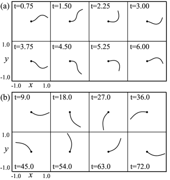
FIG. 2.: Numerical simulation of (1). (a)The clamped tube undergoes a Hopf bifurcation and begins to flutter. $N=10$, $\alpha=0.004$, $\beta=0.3$, $\gamma=1.0$. (b) The hinged tube undergoes a pitchfork bifurcation involving a Goldstone mode and begins to rotate. $N=10$, $\alpha=0.004$, $\beta=0.09$, $\gamma=1.0$.

Figure 3 shows that the critical values $\epsilon_{c}(N)$, $\omega_{c}(N)$, and $\epsilon_{h}(N)$ found numerically converge to the theoretical values $\epsilon_{c}$, $\omega_{c}$, and $\epsilon_{h}$ as $N\to\infty$. We calculated $\epsilon_{c}(N)$, $T_{c}(N)\equiv 2\pi/\omega_{c}(N)$, and $\epsilon_{h}(N)$ with 1% accuracy for several values of $N$. The data points can be fit to within the uncertainty on each data point by the function $a/(N-b)+c$, where $a$, $b$, and $c$ are the fitting parameters. From this fitting we obtain the limiting values $\epsilon_{c}(N)\to 38.0\pm 0.9$, $\omega_{c}(N)\to 195.2\pm 4.1$, and $\epsilon_{h}(N)\to 20.3\pm 0.6$ as $N\to\infty$. These are almost identical to the theoretical values, 37.69…, 191.25…, and 20.16…. Thus, we can say that the conjecture based on the results of linear stability analysis are confirmed by the numerical simulation. Moreover, we confirmed numerically that both bifurcations are supercritical by examining $\epsilon$ dependency of the magunitude of deformation.

Let us close this Letter with some supplementary comments. If the inertial terms should be considered, there are two essential parameters in the equation of motion, rather than just one. This fact suggests that the behavior of an inertial tube may be much more complex. Indeed, numerical simulations suggest that, while the inertial terms do not change the qualitative properties of the first bifurcations, they do change the subsequent bifurcations. In particular, the clamped inertial tube exhibits a period doubling route to chaos, while the hinged inertial tube undergoes a Hopf bifurcation as a second bifurcation and then exhibit a period doubling route to chaos. Such bifurcations are not observed in the case of a non-inertial tube.

An interesting feature of our model is that is relevant to both aspirating and discharging tubes[8]. In our model, the flow force is due only to the change in the momentum of the fluid at each point of the tube. The behavior exhibited by our model thus provides a prediction for both a discharging tube and an aspirating tube.

The authors are grateful to Y. Kuramoto, K. Sekimoto, S. Toh, G. Paquette and T. Miyoshi for informative discussions.

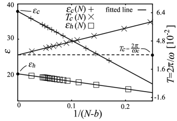
FIG. 3.: The critical values of the discrete model, $\epsilon_{c}(N)$, $T_{c}(N)\equiv 2\pi/\omega_{c}(N)$, and $\epsilon_{h}(N)$, plotted as function of $1/(N-b)$, where $b=-0.9012$, $1.9353$, and $0.1126$, respectively, are obtained from the fit. The intersections of the fitted lines and the $1/(N-b)=0$ axis correspond to the $N\to\infty$ limit. The uncertainty of the data is much smaller than the size of symbols in this plot.

REFERENCES

- [1] Email address: s_ shima@ton.scphys.kyoto-u.ac.jp
- [2] M. P. Paidoussis, Applied Mechanics Reviews 40, 163 (1987).
- [3] T. B. Benjamin Proc. R. Soc. London, Ser. A 261, 457 (1961).
- [4] R. W. Gregory and M. P. Paidoussis, Proc. R. Soc. London, Ser. A 293, 512 (1966); 293, 528 (1966).
- [5] J. Rousselet and G.Herrmann, Journal of Applied Mechanics 48, 943 (1981).
- [6] A. K. Bajaj and P. R. Sethna, Society for Industrial and Applied Mathematics 44, 270 (1984).
- [7] Wang Zhongmin and Zhao Fengqun, Acta Mechanica solid Sinica 13, 262 (2000).
- [8] Cui Hongwu and Tani Junji, JSME International Journal, Series C 39, 20 (1996).