Quasi-solitons and asymptotic multiscaling in shell models of turbulence

Abstract

A variation principle is suggested to find self-similar solitary solutions (reffered to as solitons) of shell model of turbulence. For the Sabra shell model the shape of the solitons is approximated by rational trial functions with relative accuracy of $O(10^{-3})$. It is found how the soliton shape, propagation time $t_{n}$ (from a shell # $n$ to shells with $n\to\infty$) and the dynamical exponent $z_{0}$ (which governs the time rescaling of the solitons in different shells) depend on parameters of the model. For a finite interval of $z$ the author discovered quasi-solitons which approximate with high accuracy corresponding self-similar equations for an interval of times from $-\infty$ to some time in the vicinity of the peak maximum or even after it. The conjecture is that the trajectories in the vicinity of the quasi-solitons (with continuous spectra of $z$) provide an essential contribution to the multiscaling statistics of high-order correlation functions, referred to in the paper as an asymptotic multiscaling. This contribution may be even more important than that of the trajectories in the vicinity of the exact soliton with a fixed value $z_{0}$. Moreover there are no solitons in some region of the parameters where quasi-solitons provide dominant contribution to the asymptotic multiscaling.

I Introduction

The qualitative understanding of many important statistical features of developed hydrodynamic turbulence (including anomalous scaling) may be formulated within the Kolmogorov-Richardson cascade picture of the energy transfer from large to small scales. For a dynamical modeling of the energy cascade one may use the so-called shell models of turbulence [1, 2, 3, 4, 5, 6] which are simplified versions of the Navier-Stokes equations. In shell models the turbulent velocity field ${\mathchoice{{\hbox{\boldmath$\displaystyle u$}}}{{\hbox{\boldmath$\textstyle u$}}}{{\hbox{\boldmath$\scriptstyle u$}}}{{\hbox{\boldmath$\scriptscriptstyle u$}}}}({\mathchoice{{\hbox{\boldmath$\displaystyle k$}}}{{\hbox{\boldmath$\textstyle k$}}}{{\hbox{\boldmath$\scriptstyle k$}}}{{\hbox{\boldmath$\scriptscriptstyle k$}}}},t)$ with wave numbers $\textstyle k$ within a spherical shell $k_{n}<k<k_{n+1}$ is usually presented by one complex function, a “shell velocity” $u_{n}(t)$. To preserve scale invariance the shell wave-numbers $k_{n}$ are chosen as a geometric progression

$$k_{n}=k_{0}\lambda^{n}\,,$$ (1)

where $\lambda$ is the “shell spacing” and $1\leq n\leq N$. The equation of motion reads $d\,u_{n}(t)/dt=Q_{n}$, where $Q_{n}$ is a quadratic form of $u_{m}(t)$ which describes interaction of neighboring shells. Clearly, shell models can be effectively studied by numerical simulations in which the values of the scaling exponents can be determined very precisely. Moreover, unlike the Navier-Stokes equations, the shell models have tunable parameters (like $\lambda$) affecting dynamical features of the of the energy transfer. This allows one to emphasize one after another different aspects of the cascade physics and to study them almost separately.

The statistics of $u_{n}$ may be described by the moments of the velocity $S_{p}(k_{n})$ which are powers of $k_{n}$

$$S_{p}(k_{n})\equiv\langle|u_{n}|^{p}\rangle\propto k_{p}^{-\zeta_{p}}\propto\lambda^{-n\zeta_{p}}\,,$$ (2)

in the “inertial range” of scales, $n_{L}<n<n_{d}$. Here $n_{L}$ is the largest shell index affected by the energy pumping and $n_{d}$ is the smallest shell index affected by the energy dissipation.

In the paper we employ our own shell model called the Sabra model[6]. Like in the Navier-Stokes turbulence the scaling exponents $\zeta_{p}$ in the Sabra model exhibit non linear dependence on $p$. Similar anomalies were found in the Gledzer – Okhitani – Yamada (GOY) model [1, 2]. However the Sabra model has much simpler correlation properties, and much better scaling behavior in the inertial range. The equations of motion for the Sabra model read:

$$\frac{du_{n}}{dt} = i\big{(}ak_{n+1}u_{n+2}u_{n+1}^{*}+bk_{n}u_{n+1}u_{n-1}^{*}$$ (5)

$$-ck_{n-1}u_{n-1}u_{n-2}\big{)}-\nu k_{n}^{2}u_{n}+f_{n}\,,$$

$$a+b+c=0\ .$$

Here the star stands for complex conjugation, $f_{n}$ is a forcing term which is restricted to the first shells and $\nu$ is the “viscosity”. Equation (5) guarantees the conservation of the “energy” $E$ and “helicity” $H$

$$E=\sum_{n}|u_{n}|^{2}\,,\ H=\sum_{n}(a/c)^{n}|u_{n}|^{2}\,,$$ (6)

in the inviscid ($\nu=0$) limit.
  
  

In this paper we will consider self-similar solutions of the Sabra shell models (5) in a form of solitary peaks – solitons. The important role of intense self-similar solitons in the statistics of high order structure function was discussed in Refs [7, 8, 9]. The two-fluid picture of turbulent statistics in shell models and corresponding “semi-qualitative” theory in the spirit of Lipatovs’ semi-classical approach[10] was suggested in Refs. [11, 12]: self-similar solitons form in and propagate into a random background of small intensity generated by a forcing which has Gaussian statistics and $\delta$-correlated in time. Accounting in the Gaussian approximation for small fluctuations around self-similar solitons the authors of [11, 12] reached miltiscaling statistics with a narrow spectrum of $z$. In the present paper the multiscaling statistics of high order correlation functions will be referred to as asymptotic multiscaling.

Our preliminary direct numerical simulations of the Sabra shell model[13, 14] shows the asymptotic multiscaling is a consequence of much reacher dynamics of shell models. For example in the $b$-interval $[-1<b<-0.7]$ and at $\lambda=2$ we indeed observe extremely intense self-similar peaks on a background of small fluctuations. Each particular peak has well defined time-rescaling exponent $z_{0}$, however from a peak to peak the value $z_{0}$ essentially varies[14]. In the region $[-0.3<b<0]$ the level of intermittency is much smaller,intense solitary events vanish, however turbulent statistics remains anomalous[14, 16]. Only at intermediate value of $b\ \approx-0.5$ we found[13] intense self-similar peaks with a narrow spectrum of dynamical exponent $z_{0}=0.75\pm 0.02$.

These observations may serve as a starting point in developing a realistic statistical theory of asymptotic multiscaling which will take into account a wide variety of relevant dynamical trajectories of the system not only in the vicinity of the well defined solitons. The present paper is a first step in this direction and is organized as follows.

The analytic formulation of the problem is presented in Sect. II. For the general reader I describe a self-similar form of solitary soliton “propagating” through the shells (II B). I derive the “basic self-similar equations” for the solitons (II C), consider the relevant boundary conditions (II D) and analyze the asymptotic form of soliton tails for infinite times (II E).

Section III is devoted to a variation procedure for the problem. I suggest in sect. III A a simple positive definite functional ${\cal{F}}(z)\geq 0$ such that the exact solution corresponds to ${\cal{F}}(z_{0})=0$. The analytic form of trial functions is discussed in sect. III B. In section III C we will see in details how the variation procedure works in the case of the “canonical” set of parameters $\lambda=2$, $b=-0.5$. The characteristic value of ${\cal{F}}(z)$, ${\cal{F}}_{0}$, is of the order of unity. The minimization of ${\cal{F}}(z)$ (with respect of the propagation time and soliton width, with proper choice of trial function without fit parameters and at experimentally found value $z_{0}=0.75$[13]) gives ${\cal{F}}_{\rm min}(0.75)\approx 0.08$. Step-by-step improvement of the approximation is reached by a consecutive addition of fit parameters which affect a shape of the soliton. With 10 shape parameters, the value of ${\cal{F}}_{\rm min}(z)$ may be as small as $10^{-3}$. The resulting “best” values of the shape parameters give approximate solutions of the basic equation (normalized to unity in their maximum) with local accuracy of the order of $10^{-3}$.

Section IV presents results of the minimization on trial rational functions (ratios of two polynomials) with 10 shape parameters, and their discussion. Firstly, in sect. IV A we compare and discuss the $z$-dependence of ${\cal{F}}_{\rm min}(z)$ for $b=-0.8\,,\,-0.5$ and $-0.3$ (at $\lambda=2$). An important observation (sect. IV B): there are interval of $z$ for which basic equations do not have self-similar solitary solutions for all times (solitons) but may be solved approximately for interval of times from $-\infty$ up to some moment in the vicinity of soliton maximum or even after it. Configurations of the velocity field in the vicinity of these solutions may be called quasi-solitons. My conjecture is that the quasi-solitons with continuous spectra of $z$ may provide even more important contribution to the asymptotic multiscaling than the contributions from the trajectories in the vicinity of an exact soliton with fixed scaling exponent $z_{0}$. The concept of quasi-solitons and proposed in this paper the dependence of their properties on $b$ allows us to reach a qualitative understanding of the behavior of intense events for various values of $b$, observed in direct numerical simulation of the Sabra model[13, 14, 16].

In concluding sect. V I summarize the results of the paper and present my understanding of a way ahead toward a realistic theory of asymptotic multiscaling for shell models of turbulence which also may help in further progress in the description of anomalous scaling in the Navier-Stokes turbulence.

II Basic Self-similar Equations of the Sabra shell model

A “Physical” range of parameters

In the inertial interval of scales the Sabra equation of motion (5) have formally five parameters: $k_{0}$, $\lambda$, $a$, $b$ and $c$. They enter in the equation in four combinations: $\lambda$, $(k_{0}\,a)$, $(k_{0}\,b)$ and $(k_{0}\,c)$, therefore by rescaling of the parameters $a,\,b$ and $c$ we get $k_{0}=1$. Without loss of generality we may consider $a>0$. A model with negative $a$ turns into model with positive $(k_{0}\,a)$ by replacing $u_{n}\to-u_{n}$. By rescaling of the time-scale $t\to(a\,t)$ we get a model with $a=1$. The arameters $a$, $b$ and $c$ are related by Eq. (5). Thus we can express $c=-(a+b)\to-(1+b)$. With this choice only two parameters of the Sabra model remain independent, $b$ and $\lambda$. By construction of the model $\lambda>1$. A typical choice $\lambda=2$ will be considered in the paper.

Note that for $(a/c)>0$ (which is $c>0$ or $b<-1$ at $a=1$) the model has two positive definite integrals of motion which are quadratic in $u_{n}$: the energy and “helicity” (6). In this case (as it was discussed in Ref. [15]) one may directly apply the Kraichnan argument for the enstropy and energy integrals of motion in 2D turbulence and conclude that in shell models fluxes of energy and “helicity” will be oppositely directed: “direct” cascade (from small to large shell numbers $n$) will have integral of motion for which large $n$ shells will dominate. Therefore for $(a/c)>1$ (which is $-2<b<-1$ at $a=1$) one expects direct cascade of “helicity” and inverse cascade of energy, like in 2D turbulence. This reasoning predicts direct cascade of energy for $(a/c)<1$ (or $b<-2$ at $a=1$). In both cases one cannot expect a statistically stationary turbulence with flux equilibrium because one of the (positive definite) integrals of motion will accumulate on first shells without a mechanism of dissipations. Therefore one expects an energy-flux equilibrium with direct cascade of energy like in 3D turbulence only for negative ratio $a/c$ (or $b>-1$ at $a=1$) when “helicity” integral is not positive definite and Kraichnan’s arguments are not applicable.

More careful analysis shows that only the region $-1<b<0$ (at $a=1$) may pretend to mimic 3D turbulence. For $b>0$ when $(-c)>a=1$ the existence of “helicity” integral (even not positive definite) leads to a period-two oscillations of the correlation functions which are increasing with $n$ and “unphysical” from the viewpoint of 3D turbulence. One can see this from the exact solution for the 3rd-order correlation function

$$S_{3}(k_{n})\equiv\mbox{Im}\left<u_{n-1}u_{n}u_{n+1}^{*}\right>\,,$$ (7)

which in the inertial interval of scales reads[6]:

$$S_{3}(k_{n})=\frac{1}{2k_{n}(a-c)}\Big{[}-\bar{\epsilon}+\bar{\delta}\Big{(}\frac{c}{a}\Big{)}^{n}\Big{]}\ .$$ (8)

Here $\bar{\epsilon}$ and $\bar{\delta}$ are fluxes of energy and “helicity” respectively. For any small ratio $\bar{\delta}/\bar{\epsilon}$ and $(c/a)<-1$ the correlator $S_{3}(k_{n})$ (and presumably many others) will have period-two oscillations which increase with $n$ . Therefore in this paper we will consider only the region

$$-1<b<0\,,$$

traditionally keeping $\lambda=2$.

B Self-similar form of “propagating” solitons

Self-similarity in our context means that solitons propagate through shells without changing their form. “Propagation” means that the time $t_{n}$ at which peak reaches its maximum increases with $n$, in other words, the larger $n$, the later peak reaches this shell. Intuitively this picture corresponds to the energy transfer from shells with small $n$ to large ones.

Self-similar propagation of the solitons may be formally described by the same function $f(\tau_{n})$ of dimensionless time $\tau_{n}$ which is counted from the time of the soliton maximum $t_{n}$ and normalized by some characteristic time for $n$th shell $T_{n}$:

$$\tau_{n}=(t-t_{n})/T_{n}\ .$$ (9)

The time $T_{n}$ has to be rescaled with $n$ as follows:

$$T_{n}=T\lambda^{-zn}\,,\quad T=1/(k_{0}\,v)\,,$$ (10)

where $z$ is a dynamical exponent and the characteristic time $T$ is organized from the characteristic velocity of the soliton $v$ and the wave vector of the problem $k_{0}$. The time delays $t_{n}-t_{n-1}$ also have to re-scale like $T_{n}$:

$$t_{n-1,n}\equiv t_{n}-t_{n-1}=\tilde{\tau}T\lambda^{-zn}\,,$$ (11)

where the positive dimensionless time $\tilde{\tau}$ is of the order of unity.

Consider next the amplitudes of the solitons. Denote as $u_{n,\rm max}$ the maximum of the velocity in the $n$th shell which also re-scales with another exponent $y$:

$$u_{n,\rm max}=v\lambda^{-yn}\ .$$ (12)

In order to relate the exponents $z$ and $y$ we sketch the basic equations (5) having in mind only dimensions and $\lambda^{n}$ dependence:

$$(du_{n}/dt)\propto k_{0}\,\lambda^{n}u_{n}^{2}\ .$$

Consequently $T_{n}^{-1}\sim k_{0}\lambda^{n}u_{n,\rm max}$  and therefore

$$y+z=1\ .$$ (13)

Finally we may write a self-similar substitution in the form:

$$u_{n}(t)=-iv\lambda^{-yn}f\left[(t-t_{n})vk_{0}\lambda^{zn}\right]\ .$$ (14)

With this choice of a prefactor $(-i)$, the real and positive function $f$ will give a positive contribution to the energy flux (7) in the inertial interval of scales:

$$\bar{\epsilon}=2k_{n}\,(a-c)\,\mbox{Im}\langle u_{n-1}^{*}u_{n}^{*}u_{n+1}\rangle\ .$$ (15)

Note that all these considerations are not specific for the Sabra model. They are based on very general features of shell models of turbulence, namely the quadratic form of nonlinearity with the amplitudes of interaction proportional to $\lambda^{n}$. In Refs. [9, 11] similar forms of the self-similar substitutions were taken for the Obukhov – Novikov and for the GOY models.

C Self-similar equation of motion

Introduce a dimensionless time for the $n$th shell as follows:

$$\tau_{n}\equiv(t-t_{n})vk_{0}\lambda^{zn}\ .$$ (16)

The right-hand side (RHS) of the equation for $d\,f(\tau_{n})/d\,\tau_{n}$ will involve a function $f$ with arguments $\tau_{n\pm 1}$ and $\tau_{n\pm 2}$. All these times may be uniformally expressed in terms of a new dimensionless time

$$\tau_{0}\equiv\tilde{\tau}/(\lambda^{z}-1)$$ (17)

as:

$$\tau_{n\pm s}=\lambda^{\pm sz}(\tau_{n}-\tau_{0})+\tau_{0}\,,\quad s=1,\,2\ .$$ (18)

The characteristic time $\tau_{0}$ is related to the time $t_{n,\infty}$ which is needed for a pulse to propagate from the $n$th shell all the way to infinitely high shells:

$$t_{n,\infty}\equiv\sum_{m=n}^{\infty}t_{m,m+1}=\tau_{0}\lambda^{-nz}\,T\ .$$ (19)

Substituting Eq. (14) in (5) and using relationship (18) one gets the “basic equation” of our problem

$$D(\tau)\equiv\frac{d\,f(\tau)}{d\tau}-C(\tau)\ .$$ (20)

Here we replaced $\tau_{n}\to\tau$ and introduced a “collision” term $C(\tau)$ according to:

$$C(\tau)\equiv-a\,\lambda^{3z-2}\,f^{*}[\lambda^{z}(\tau-\tau_{0})+\tau_{0}]\,f[\lambda^{2z}(\tau-\tau_{0})+\tau_{0}]$$ (21)

$$-\,\,c\lambda^{2-3z\,}f[\lambda^{-z}(\tau-\tau_{0})+\tau_{0}]\,f[\lambda^{-2z}(\tau-\tau_{0})+\tau_{0}]$$ (22)

$$+(a+c)\,f^{*}[\lambda^{-z}(\tau-\tau_{0})+\tau_{0}]\,f\,[\lambda^{z}(\tau-\tau_{0})+\tau_{0}]\ .$$ (23)

D Boundary conditions of the basics equation (20)

The boundary conditions at $\tau=\pm\infty$ for a soliton are obvious:

$$f(\pm\infty)=0\ .$$ (24)

By construction the soliton reaches a maximum at $\tau=0$. Therefore

$$\frac{df(\tau)}{d\tau}\Big{|}_{\tau=0}=0\ .$$ (25)

Introduce a characteristic width of a soliton $1/d$ according to

$$\frac{d^{2}\,f(\tau)}{d\,\tau^{2}}\Big{|}_{\tau=0}=-d^{2}\ .$$ (26)

It is convenient to introduce a new time variable $s$ and a function $g(s)$ with the unit width:

$$f(\tau)\equiv g(s)\,,\quad s\equiv\tau\,d\,,$$ (27)

$$\frac{d^{2}\,g(s)}{d\,s^{2}}\Big{|}_{s=0}=-1\ .$$ (28)

With this time variable, the equation of motion (20) reads

$${\cal{D}}(s,z,s_{0},d)=q(s)-{\cal{C}}(s,z,s_{0})=0\,,$$ (29)

where

$$~{}\qquad q(s)\equiv d\,\frac{d\,g(s)}{ds}\,,\qquad s_{0}\equiv\tau\,d\,,$$ (30)

$${\cal{C}}(s,z,s_{0})\equiv(a+c)\,g^{*}\big{(}\frac{s-s_{0}}{\lambda^{z}}+s_{0}\big{)}\,g\,[\lambda^{z}(s-s_{0})+s_{0}]$$ (31)

$$-a\,\lambda^{3z-2}\,g^{*}[\lambda^{z}(s-s_{0})+s_{0}]\,g[\lambda^{2z}(s-s_{0})+s_{0}]$$ (32)

$$-\,\,c\lambda^{2-3z\,}g\big{(}\frac{s-s_{0}}{\lambda^{z}}+s_{0}\big{)}\,g\big{(}\frac{s-s_{0}}{\lambda^{2z}}+s_{0}\big{)}\,,$$ (33)

Function $g(s)$ should vanish at infinite times:

$$\lim_{s\to-\infty}g(s) = 0\,,$$ (34)

$$\lim_{s\to\infty}g(s) = 0\ .$$ (35)

The boundary conditions at $s=0$ read:

$$g(0)=1\,,\quad\frac{d\,g(s)}{d\,s}\Big{|}_{s=0}=0\,,\quad\frac{d^{2}\,g(s)}{d\,s^{2}}\Big{|}_{s=0}=-1\ .$$ (36)

Note that the problem to find a form of the self-similar solitons may be divided into two independent problems: for times smaller and larger than $s_{0}$. Indeed, Eq. (29) for times $s<s_{0}$ does not contain functions for times $s>s_{0}$ and vice versa. At the boundary between these regions Eq. (29) reduces to

$$\frac{d}{d\,s_{0}}\Big{[}\frac{1}{g(s_{0})}\Big{]} = d\,p_{0}\,,$$ (37)

$$p_{0} = a(\lambda^{3z-2}-1)-c(1-\lambda^{2-3z})\ .$$ (38)

In our discussion $a>0$, $c<0$, $\lambda>1$ and $z>2/3$. Therefore $p_{0}>0$ and $d\,g(s_{0})/d\,s_{0}<0$. It means that the time $s_{0}$ is larger than the time $s=0$ at which $g(s)$ has a maximum, i.e. $s_{0}>0$. As we noted [and see Eq. (19)], $s_{0}$ is the time which is needed for a pulse to propagate from the $n$th shell to infinity high shell. Therefore the relation $s_{0}>0$ agrees with our understanding of the direct cascade.

So, we will divide the time interval $[-\infty<s<\infty]$ into two subintervals: $[-\infty<s\leq s_{0}]$ and $[s_{0}<s<\infty]$. For $[-\infty<s\leq s_{0}]$ the maxima of the solitons in all shells are in the inertial interval of scales and very high shells are not yet activated. We will refer to this interval as an inertial interval of times. In the second time interval, for $s>s_{0}$ high-shell solitons already reached the dissipative interval of scales. We will refer to this interval as a dissipative interval of times. Generally speaking, in this interval one has to account for the viscous term in the equation of motion. In this paper we will restrict ourselves to the inertial interval of times.

It was shown in Ref. [9] that equations similar to (20) with similar boundary conditions can be considered as nonlinear eigenvalue problems. They have trivial solutions $f(s)=0$, but they may have nonzero solutions for particular the values of $z=z_{0}$ and $s_{0}$. Below we will find nontrivial solutions of our Eq. (29) that satisfies conditions (34), (36) and for which $z_{0}$ lies in the physical region $\frac{2}{3}<z<1$.

E Qualitative analysis of self-similar solutions at $s\to\pm\infty$

In this subsection we will analyze time dependent solutions of (5) which are more general than a Kolmogorov-41 (K41) and have a form of solitary pulses – solitons. We will show that the solitons have long (power-like) tails $g(s)\propto s^{x_{\pm}}$ at $s\to\pm\infty$. One way to find the asymptotic solution of Eq.  (29) is to balance the exponents in its left-hand side (LHS) and RHS. For $g(s)\propto s^{-x}$ this gives immediately $x=1$. Thus: $g(s)=D_{1}/s$. Equating prefactors in the LHS and RHS of the Eq. (20) we get:

$$D_{1}=\frac{-\lambda^{2}\,d}{(a-c\lambda^{2})(\lambda^{2}-1)}\ .$$ (39)

The coefficient $D_{1}$ appeared to be real and, in the actual range of the parameters ($\lambda>1\,\ a>0\,,\ c<0$), negative. For the positive function $g(s)$ this asymptotic form describes the front part of the pulse (at negative $s$). So:

$$g(s)=\frac{-\lambda^{2}\,d}{s(a-c\lambda^{2})(\lambda^{2}-1)}\,,\quad s\to-\infty\ .$$ (40)

Another approach is to assume that in the equation $[g(s)\propto s^{-x}]$ the exponent $x<1$. Then, the LHS will behave as $1/s^{1+x}$ while the RHS will be proportional to $1/s^{2x}$. In the limit $s\to\infty$ and at $x<1$ one may neglect the LHS of the Eq. (29). Then the exponent $x$ cannot be found by power-counting. Instead one requires that the prefactor in the RHS [i.e. in the ${\cal{C}}(s)$ term] must vanish. This gives the following equation for $x$:

$$0=a\lambda^{3z(1-x)-2}+c\lambda^{2-3z(1-x)}-(a+c)\ .$$ (41)

Denoting

$$\Lambda\equiv\lambda^{3z(1-x)-2}\,,$$ (42)

we have, instead of Eq. (41), the square equation for $\Lambda$:

$$a\Lambda^{2}-(a+c)\Lambda+c=0\,,$$

with the roots

$$\Lambda_{1}=1\,,\ \ \Lambda_{2}=c/a\ .$$

In the chosen region of parameters ($c$ and $a$ have different signs) $\Lambda_{2}<0$, which contradicts the assumption of real $x$. Therefore the only root $\Lambda_{1}=1$ is relevant. According to definition (42) this gives

$$x_{1}=\gamma\equiv 1-\frac{2}{3z}\ .$$ (43)

Here we used notation $\gamma$ for the exponent of the long positive tail of the pulse introduced in[9] for the Novikopv-Obukhov shell model. As we see, the relation (43) is model independent. Actually this equation is a consequence of the conservation of energy (reflected in the constraint $a+b+c=0$) and the fact that the shell models account only for interaction of three consequent shells. Clearly, the relevant region of $\gamma$ is $0<\gamma<1$. This corresponds to

$${2\over 3}<z<1\ .$$ (44)

We conclude that for $s\to+\infty$

$$g(s)=D_{\gamma}/s^{\gamma}\,,$$ (45)

with a free factor $D_{\gamma}$ which has to be determined by matching the asymptotics (45) with a solution in the region $s\sim s_{0}$. It is known [8] that the self-similar core of the function $g(s)$ gives rise to a linear $n$-dependence of the scaling exponent $\zeta_{n}$ of the $n$th order structure function at large $n$:

$$\zeta_{n}=z+(1-z)n\,,\quad\mbox{at}\ n>n_{\rm cr}=1/\gamma\ .$$ (46)

For $z=\frac{2}{3}$ Eq. (45) gives the K41 slope $\frac{1}{3}$ which is the largest possible one. Value $z=1$ corresponds to the largest possible intermittency (zero slope). Therefore we may consider Eq. (44) as the “physical region” of the dynamical exponent $z$.

III Variation procedure for solitons and quasi-solitons

A Suggested functionals

Consider the following functional acting on the function $g(s)$

$${\cal{F}}\{g(s)|z,s_{0},d\}\equiv\sqrt{\int_{-\infty}^{s_{0}}d\,s[{\cal{D}}(s,z,s_{0},d)]^{2}}\,,$$ (47)

which also depend on the parameters of the problem $\lambda$, $b$, $z$, $s_{0}$ and $d$. By construction, the functional ${\cal{F}}\{g(s)|z,s_{0},d\}$ is non-negative and equal zero if $g(s)$ is a solution of the problem (29): ${\cal{D}}=0$. Clearly, the functional (47) is not unique. For example, we may use more general, “weighted” functional,

$$\tilde{\cal{F}}\{g(s)|z,s_{0},d\}\equiv\sqrt{\int_{-\infty}^{s_{0}}d\,sW(s)[{\cal{D}}(s,z,s_{0},d)]^{2}}\,,$$ (48)

with some positive “weight” function $W(s)>0$. This functional is also positive definite and also equal zero if $g(s)$ is a solution of the problem (29).

One can easily find many other functionals giving approximate solutions of the problem. The functional ${\cal{F}}\{g(s)|z,s_{0},d\}$ has an advantage of simplicity. Its minimization (with a proper choice of the trial function) leads to a solution of the problem with hight accuracy. For example, with trial functions discussed in Section III B the relative accuracy (with respect to the value of a soliton maximum) is $O(10^{-3})$. Therefore we will restrict the present discussion to the simple functional ${\cal{F}}\{g(s)|z,s_{0},d\}$.

B Suggested form of trial functions

For simplicity, in this paper we will seek only real (without nontrivial phases) solitons. Complex solitons will be discussed (within the same scheme) elsewhere.

My suggestion is to use different trial functions for negative and positive times, both satisfying boundary conditions (36) at $s=0$. Denote as $g_{m+}(s)$ the trial functions for positive times with $m$ shape parameters. Let the function $g_{m+}(s)$ satisfy condition (37) at $s=s_{0}$. This condition is a constraint on the time derivative of $1/g_{m+}(s)$. Having also in mind that $g_{m+}(s)$ is defined on the interval $[0<s<s_{0}]$ with $s_{0}\sim 1$ it is convenient to choose $1/g_{m+}(s)$ as a polynomial in $s$. The first (free) term of expansion is 1 because $g_{m+}(0)=1$. The second term ($\propto s$) vanishes due to $dg(s)/ds=0$ at $s=0$. The next term must be $s^{2}/2$ due to the restriction on the second derivative (36) at $s=0$. In order to satisfy condition (37) at $s=s_{0}$ we have to account at least for a cubic term. Therefore the simplest function of this type, $g_{0+}(s)$ without fit parameters takes the form

$$g_{0+}(s)\equiv\Big{[}1+\frac{s^{2}}{2}+\frac{s^{3}}{3s_{0}^{2}}\Big{(}\frac{p_{0}}{d}-s_{0}\Big{)}\Big{]}^{-1}\ .$$ (49)

If needed we can add fit parameters $p_{1}$, $p_{2}$, etc. accounting for terms $\propto s^{4}$, $\propto s^{5}$, etc. Accordingly, a trial function with $m$ shape parameters takes the form:

$$g_{m+}(s) = \Big{[}1+\frac{s^{2}}{2}+\frac{s^{3}}{3s_{0}^{2}}\Big{(}\frac{p_{0}}{d}-s_{0}-\sum_{j=1}^{m}p_{j}\Big{)}$$ (51)

$$+\sum_{j=1}^{m}\frac{p_{j}\,s^{j+3}}{(j+3)\,s_{0}^{j+2}}\Big{]}^{-1}\ .$$

In most cases it would be enough to use $g_{5+}(s)$ with 5 shape parameters.

Denote as $g_{m-}(s)$ the trial functions for negative times having $m$ shape parameters. These functions have to approximate the basic equation on the infinite time interval from $-\infty$ to $0$. Therefore their analytic form is a much more delicate issue. Analyzing the form of the peaks observed in direct numerical simulations[14]. I have found a function $\tilde{g}_{1-}(s)$ with one fit parameter $q$,

$$\tilde{g}_{1-}(s)\equiv\frac{1-s\sqrt{q/(q-1)}}{\big{[}1-s/\sqrt{q(q-1)}\,\big{]}^{q}}\,,$$ (52)

which allows us to reach accuracy of solution of Eq. (29) of $O(10^{-2})$. This accuracy would be enough for future comparison of the “theoretical” shape of a pulse with that found in direct numerical simulation of the Sabra model. However this function does not have the correct asymptotic behavior (40) for $s\to-\infty$ and is inconvenient for successive improvements of the approximation.

Instead of $\tilde{g}_{1-}(s)$ for negative time I use in the regular minimization procedure a ratio of two polynomials of $n$th and $n+1$ orders. This ratio has $2n+2$ free parameters. After accounting for three conditions (36), just $(2n-1)$ parameters remain free. Simple function of this type with $n=1$, which also agrees with asymptotic (40), has no free parameters:

$$\tilde{g}_{0-}(s)=\frac{2+D_{1}s}{2+D_{1}s+s^{2}}\ .$$ (53)

We will discuss even more simple rational function

$$g_{0-}(s)=[1+\frac{1}{2}s^{2}]^{-1}\ .$$ (54)

Actually a better approximation may be achieved by a function similar to (53) with one free parameter $q_{1}$:

$$g_{1-}(s)=\frac{1+q_{1}s}{1+q_{1}s+\frac{1}{2}s^{2}}\ .$$ (55)

In actual calculations it would be sufficient for our purposes to account for 5 shape parameters in the function:

$$g_{5-}(s)=\frac{1+q_{1}s+q_{2}s^{2}+q_{4}s^{3}}{1+q_{1}s+(q_{2}+\frac{1}{2})s^{2}+q_{3}s^{3}+q_{5}s^{4}}\ .$$ (56)

The function $g_{5-}(s)$ reduces to $g_{3-}(s)$ by choosing $q_{4}=q_{5}=0$ and to $g_{1-}(s)$ at $q_{2}=q_{3}=q_{4}=q_{5}=0$.

C Test of the variation procedure

In this subsection we will see in detail how the variation procedure suggested above works for the “canonical” set of parameters $\lambda=2$, $b=-0.5$. Denote as ${\cal{F}}_{{\rm min},m}(z)$ the result of a minimization of the functional ${\cal{F}}\{g(s)|z,s_{0},d\}$ acting on the functions $g_{m\pm}(s)$ at given $z$. The parameters in the minimizations are: the propagation time $s_{0}$, width parameter $d$, $m$ shape parameters for negative times ($q_{1},\cdots q_{m}$) and $m$ shape parameters for positive times ($p_{1},\cdots p_{m}$):

$${\cal{F}}_{{\rm min},m}(z)\equiv\min_{q_{j},p_{j}|s_{0},d}{\cal{F}}\{g(s)|z,s_{0},d\}\ .$$ (57)

Table 1 displays the found values of ${\cal{F}}_{{\rm min},m}(z)$ for $z=0.75,\,0.85$, $0.95$ and $m=0$, 1, 3, 5.

Consider first the case $z=0.75$, which corresponds to the dynamical exponent ofintense self-similar peaks observed in our direct numerical simulation of the Sabra shell model [13]. At $m=5$ we have reached ${\cal{F}}_{\rm min,5}(0.75)\approx 2.3\cdot 10^{-4}$. This value is more than 200 times smaller than characteristic value of the functional before minimization, ${\cal{F}}_{0}\approx 0.5$. This allows us to hope that the minimization using the functions $g_{5\pm}(s)$ with total number $2\,m=10$ of the shape parameters will be sufficient for most applications.

Note that for some purposes we may use less then 10 shape parameters. For example “optimal” values of $s_{0}$ and $d$ shown in the Table 1 begin to converge for $m\geq 3$. Therefore for a reasonable good estimate of $s_{0}$ and $d$ we may use the trial functions $g_{3\pm}(s)$ having 6 shape parameters. Moreover, the same level of accuracy as with $m=3$ may be achieved just with two shape parameters ($q,\,p_{1}$) if we replace $g_{3-}(s)$ by $\tilde{g}_{1-}(s)$ and, (which is less important) $g_{3+}(s)\to g_{1+}(s)$. Minimization with $\tilde{g}_{1-}(s)$ and $g_{1+}(s)$ gives:

$$\min_{s_{0},d,q,p_{1}}{\cal{F}}\{g(s)|z,s_{0},d\}\approx 0.0197\,,\ \mbox{at}\ z = 0.75\,,$$ (58)

$$s_{0}\approx 0.54\,,\ d\approx 1.57\,,\ q\approx 8.59\,,\ p_{1} \approx -0.44\ .$$ (59)

Another example in which we may use less then 10 shape parameters for a reasonable good description is the shape of solitons, $g(s)$. Fig. 1 displays functions $g(s)$ and $q(s)$, Eq. (30) for $m=3$ (dashed lines) and for $m=5$ (solid lines). We see that for comparison with experiments we can use simpler form with $m=3$. In Fig. 1 are also plotted by dashed lines functions $g(s)$ and $q(s)$ resulting from minimization (58) with 2 shape parameters. They are indistinguishable from the corresponding functions having 6 shape parameters.

Table 1. Optimal values of $(s_{0},\,d)$ for $z=0.75$ and  values of ${\cal{F}}_{{\rm min},m}$ for $z=0.75,\,0.85$ and $0.95$. Number of the shape parameters $m=0,\,1,\,3$ and 5.

		$~{}m=0~{}$	$~{}m=1~{}$	$~{}m=3~{}$	$~{}m=5~{}$
$z=0.75$	$s_{0}$	0.36	0.36	0.55	0.517
$z=0.75$	$~{}d$	1.19	1.18	1.59	1.49
$z=0.75$	${\cal{F}}_{{\rm min},m}$	0.0811	0.0675	0.0176	0.00234
$z=0.85$	${\cal{F}}_{{\rm min},m}$	0.2047	0.1014	0.0284	0.0092
$z=0.95$	${\cal{F}}_{{\rm min},m}$	0.3471	0.1377	0.0780	0.0650

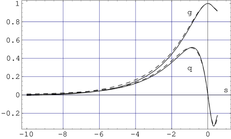
FIG. 1.: Trial functions $g(s)$ and $q(s)\equiv d[dg(s)/ds]$ for $\lambda=2$, $b=-0.5$ and $z=0.75$. Solid lines correspond to the full minimization ($m=5$), dashed – to $m=3$. The same dashed lines show results of the minimization (58) with only two shape parameters.

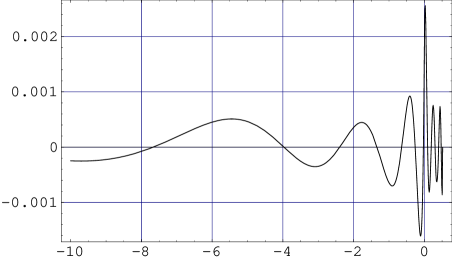
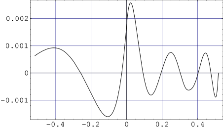
FIG. 2.: Local deviation ${\cal{D}}_{{\rm min},5}(s,0.75)$, Eq. (29) vs $s$ for $\lambda=2$, $b=-0.5$. Upper panel: region $-10<s<s_{0}$. Lower panel: blow up of the region $-s_{0}<s<s_{0}$.

Note that the minimal values of the functional ${\cal{F}}_{{\rm min},m}(z)$ characterize the “global” accuracy of the approximation in the whole interval of $s$, [$\infty\,,\ s_{0}$]. It would be elucidative to discuss a “local deviation” which may be described by the function ${\cal{D}}(s,z,s_{0},d)\equiv q(s)-{\cal{C}}(s,z,s_{0})$.

According to Eq. (29), the local deviation ${\cal{D}}(s,z,s_{0},d)$ has to vanish for all $s$. Denote as ${\cal{D}}_{{\rm min},m}(s,z)$ the deviation ${\cal{D}}(s,z,s_{0},d)$ at optimal values of $s_{0},d$ and $2m$ shape parameters. The deviation ${\cal{D}}_{{\rm min},5}(s,0.75)$ is shown in Fig. 2. Excluding the small region $|s|<0.1$ the deviation ${\cal{D}}_{{\rm min},5}(s,0.75)<10^{-3}$, i.e. in more than 500 times smaller than the maximal value of $q(s)$ shown in Fig. 1. This serves for us as a strong support of the conjecture that by adding more and more fit parameters one can reach smaller and smaller values of ${\cal{F}}_{{\rm min}}$, i.e. $\lim_{m\to\infty}{\cal{F}}_{{\rm min},m}=0$ and for $z=0.75$ one can find a true solution of the problem. The currently available personal computers allow to find solutions with ${\cal{F}}_{{\rm min},10}\sim 10^{-3}$ and ${\cal{D}}<2\cdot 10^{-3}$ during one-two hours of calculations using the standard package of Wolfram’ Mathematica.

Consider now different a value of $z=0.95$. As follows from the Table 1, there are no jumps in improving the approximation for $m\geq 2$. For $z=0.95$ the ratio ${\cal{F}}_{{\rm min,1}}(z)/{\cal{F}}_{{\rm min,5}}(z)\simeq 2$ while for $z=0.75$ the same ratio ${\cal{F}}_{{\rm min,1}}(z)/{\cal{F}}_{{\rm min,5}}(z)\simeq 28$. It is very reasonable to expect that ${\cal{F}}_{{\rm min},m}(0.95)$ cannot be much smaller that 0.06 even for very large $m$. One may conclude that for $z=0.95$ there is no “global” solution in the interval $[-\infty<s<s_{0}]$.

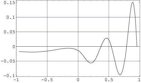
FIG. 3.: Local deviation ${\cal{D}}_{{\rm min},5}(s,0.95)$ vs $s$ for $\lambda=2$, $b=-0.5$ and $z=0.95$ with optimal set of 10 shape parameters. Upper panel: region $-10<s<s_{0}$. Lower panel: blow up of the region $-s_{0}<s<s_{0}$.

Nevertheless, the local deviation ${\cal{D}}_{{\rm min},5}(s,0.95)$ shown in Fig. 3 is quite small, say in the region $s<0$. Moreover, in the region $s<s_{*}\approx-2$ the characteristic value of the deviation ${\cal{D}}_{{\rm min},5}(s,0.95)$ is more or less the same as for $z=0.75$ where we have approximate solution (soliton) in the whole region $s<s_{0}$. Consequences of this fact will be discussed later.

IV Solitons, quasi-solitons and Asymptotic Multiscaling

A $z$-valleys of the functional ${\cal{F}}_{{\rm min,5}}(z)$

In this section we discuss the $z$-dependence of the functional ${\cal{F}}_{{\rm min},5}(z)$ and of the optimal values of $s_{0}$ and $d$. These functions for $b=-0.5$, $-0.8$, $-0.3$ are displayed in Figs. 4, 5,  6 respectively.

For $b=-0.5$ (Fig. 4) the $z$-dependence of the functional has a minimum ${\cal{F}}_{{\rm min,5}}(z)\approx 2\cdot 10^{-3}$ around $z\approx 0.734$. This minimum is quite flat. For example, ${\cal{F}}_{{\rm min,5}}(z)<{\cal{F}}_{*}\equiv 2.5\cdot 10^{-3}$ for $z$ within the interval $[z_{\rm min}=0.71,z_{\rm max}=0.76]$. Note that for $b=-0.8$, (Fig. 5) the same (arbitrary) level ${\cal{F}}_{*}$ exceeds ${\cal{F}}_{{\rm min,5}}(z)$ for $z$ in the wider interval $[0.71,0.84]$. In the same time for $b=-0.3$ (Fig. 6) there are no values of $z$ for which ${\cal{F}}_{{\rm min,5}}(z)<{\cal{F}}_{*}$. A natural interpretation of these facts

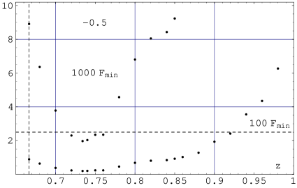
FIG. 4.: The $z$ dependence of $10^{3}{\cal{F}}_{{\rm min,5}}$, $10^{2}{\cal{F}}_{{\rm min,10}}$ (Upper panel) and $s_{0}$,  $d$ (Lower panel) for $\lambda=2$, $b=-0.5$. Vertical dashed lines shows K41 value of $z=2/3$. Horizontal dashed line in upper panel corresponds to chosen value $10^{3}{\cal{F}}_{*}=2.5$. Points for $10^{3}{\cal{F}}_{{\rm min,5}}$ with $0.72<z<0.76$ are below this level.

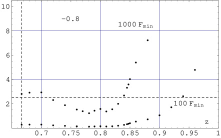
FIG. 5.: The $z$ dependence of $10^{3}{\cal{F}}_{{\rm min,5}}$, $10^{2}{\cal{F}}_{{\rm min,5}}$ (Upper panel) and $s_{0}$,  $d$ (Lower panel) for $\lambda=2$, $b=-0.8$. Vertical dashed line shows K41 value of $z=2/3$. Horizontal dashed line in upper panel corresponds to chosen value $10^{3}{\cal{F}}_{*}=2.5$. Points for $10^{3}{\cal{F}}_{{\rm min,5}}$ with $0.71<z<0.84$ are below this level.

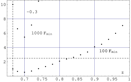
FIG. 6.: The $z$ dependence of $10^{3}{\cal{F}}_{{\rm min,5}}$, $10^{2}{\cal{F}}_{{\rm min,10}}$ (Upper panel) and $s_{0}$,  $d$ (Lower panel) for $\lambda=2$, $b=-0.3$. The vertical dashed line shows K41 value of $z=2/3$. Horizontal dashed line in upper panel corresponds to chosen value $10^{3}{\cal{F}}_{*}=2.5$. All points for $10^{3}{\cal{F}}_{{\rm min,5}}$ exceed this level.

is that at $b=-0.8$ one can meet in the velocity realization (of the Sabra model) $u_{n}(t)$ intense solitons with values of $z$ in a quite wide interval (for example in the interval [0.71, 0.84] mentioned above), at $b=-0.5$ “allowed” interval of $z$ is more narrow (say, [0.71, 0.76]) and for $b=-0.3$ one hardly can meet intense solitons at all. As we will discuss below this statement is in a quantitative agreement with the preliminary results of the numerics [14].

Clearly, we are not talking about particular values of $z_{\rm min}$ and $z_{\rm max}$, for example because the boundary level ${\cal{F}}_{*}=2.5\cdot 10^{-3}$ was chosen arbitrarily. Moreover, the objects $z_{\rm min}$, $z_{\rm max}$ do not have explicit sense. The actual conjecture is that the functional ${\cal{F}}_{{\rm min},m}(\lambda,b,z)$ is correlated with a probability to meet a soliton or quasi-soliton with given dynamical exponent $z$ in the realization (for given $\lambda$ and $b$): the smaller value of ${\cal{F}}_{{\rm min},m}(z)$ (at large enough $m$), the larger this probability. From this point of view the two following scenarios are statistically almost equivalent. The first one may be called a multi-soliton scenario: there is a discrete spectrum of solitons with some close set of exponents $z_{0,1}$, $z_{0,2}$ in the interval $[z_{\rm min}$, $z_{\rm max}]$. One can imagine that this is the case by looking at Fig. 5 (upper panel) where the function ${\cal{F}}_{{\rm min,5}}(2,-0.8,z)$ has two minima at $z_{0,1}\approx 0.77$ and $z_{0,2}\approx 0.81$. The second one will be referred to as a quasi-soliton scenerio with continuous $z$-spectrum of quasi-solitons in some (wide) interval of $z$.

B Local deviations and quasi-solitons

The analysis of the local deviations ${\cal{D}}_{{\rm min},m}(s,z)$ presented in this section supports a quasi-soliton scenario of asymptotic multiscaling. Let us chose $b=-0.8$ for which we found in Fig. 5, (upper panel) the wide deep $z$-valley of the functional ${\cal{F}}_{{\rm min},5}(z)$. Compare the $s$-dependence of ${\cal{D}}_{{\rm min},m}(s,z)$ for the value of $z=0.81$, which corresponds to the right local minimum of the functional and for two slightly larger values of $z=0.84$ and 0.88. The local deviations ${\cal{D}}_{{\rm min},m}(s,z)$ are plotted in Fig. 7 for $z=0.81$ by solid lines, for $z=0.84$ by dashed lines and for $z=0.88$ by dash-dotted lines. The upper panel shows $s$-interval of a left tail the soliton up to its maximum: $[-10<s<0]$. The lower panel shows $s$-interval around soliton maximum: $[-1<s<s_{0}]$.

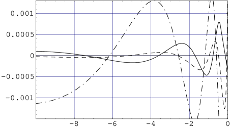
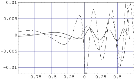
FIG. 7.: Local deviation ${\cal{D}}$, Eq. (29) vs $s$ for $\lambda=2$ and $b=-0.8$. Upper panel: region $-10<s<0$. Lower panel: region $-1<s<s_{0}$. Solid lines: $z=0.81$, dashed lines: $z=0.84$, dash-dotted lines: $z=0.88$.

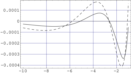
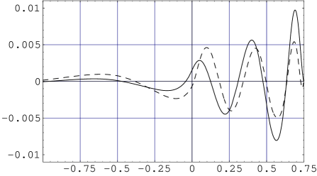
FIG. 8.: Local deviation ${\cal{D}}$, Eq. (29) vs $s$ for $\lambda=2$, $b$=-0.8 and $z=0.84$. Solid lines-results of minimization of the functional (47) with unite weight, dashed lines- the same with the weighed functional (48), (60). Upper panel: region $-10<s<-1$. Lower panel: region $-1<s<s_{0}$.

It was mentioned that the value $z_{0,2}=0.81$ corresponds to the right local minimum of the functional. The local deviation $|{\cal{D}}_{{\rm min,5}}(s,0.81)|$ is about $2\cdot 10^{-3}$ in the $s$-region $[-1,s_{0}]$, see solid line in Fig. 7, lower panel). For $s<-2$ (the upper panel) the local deviation is almost 10 times smaller, about $2.5\cdot 10^{-4}$. The value $z=0.84$ does not correspond to $z$-minima of the functional: ${\cal{F}}_{{\rm min,5}}(0.84)\approx 2\,{\cal{F}}_{{\rm min,5}}(0.81)$. The larger value of ${\cal{F}}_{{\rm min,5}}(0.84)$ is mostly determined by the region of positive $s$ where $|{\cal{D}}_{{\rm min,5}}(s,0.84)|$ exceeds 0.01, which essentially larger than the local deviations in this region at $z=0.81$, [compare dashed ($z=0.84$) and solid ($z=0.81$) lines in the lower panel of Fig. 7]. Unexpectedly, in the region $s<-1$ (the upper panel) the local deviation at $z=0.84$ even smaller than that at $z=z_{0,2}=0.81$. In other words, in this $s$-region the reached approximation is better for value $z=0.84$ than that for $z=0.81$. Dash-dotted lines in Fig. 7 show that the local deviation for a $z=0.88$ essentially larger than for $z=0.84$ and $0.81$.

Let us show that these qualitative results are independent of the particular form of the functional (47) which we chose. For that consider the weighed functional (48) with the weight fuction:

$$W(s)=[(s-s_{0})^{2}+1]^{y}\,,$$ (60)

which is of the order of unity in the vicinity of the soliton maximum and increases toward the front tail as $|s|^{2y}$. At $y=0$ one recovers the uniform weight $W(s)=1$. For positive $y$ the weight function emphasize the left tail, i.e. the region $s\ll 1$. The value of $y$ has to be smaller than $\frac{1}{2}$, otherwise the $s$-integral in (48) diverges. It is reasonable to choose an intermediate value of $y=1/4$ and to repeate the minimization procedure. The resulting changes in the values of $s_{0}$, $d$ and shape parameters were minor. For example (for $\lambda=2$, $b=-0.8$, $z=0.84$) $s_{0}=0.7506\to 0.7478$, $d=1.2645\to 1.2618$. Fig. 8 compares the local deviation ${\cal{D}}$ for unweighed (solid lines) and weighed (dashed lines) functionals. Again, the difference between these two approaches is minor.

A natural interpretation of all these facts as is follows: for some discrete values of $z=z_{0,j}$ (say for $z_{0,1}\approx 0.734$ at $b=-0.5$ and $z_{0,1}\approx 0.78$, $z_{0,2}\approx 0.81$ at $b=-0.8$) the variation procedure allows to find better and better approximation to the solution in the global sense: ${\cal{F}}_{{\rm min},m}(z_{0,j})\to 0$ in the limit $m\to\infty$. Clearly in these cases solution $g(s)$ exists also locally: the maximum of the local deviation ${\cal{D}}_{{\rm min},m}(s,z_{0,j})$ also goes to zero in this limit. In means that there are self-similar solitons in the shell model with scaling exponents $z_{0,j}$. For other values of $z$ there is no global solution. It means that for $m\to\infty$ limit of ${\cal{F}}_{{\rm min},m}$ is finite, but may be small enough. Nevertheless for a wide region of $s<s_{*}$ (in the example $z=0.75$, $b=-0.5$ the value of $s_{*}\approx-2$) the local deviation ${\cal{D}}_{{\rm min},m}(s,z)$ is very small and equation (29) may be “almost solved”. We may say that the variation procedure finds “quasi-solutions”, which approximate the equations of motion with very good accuracy starting from the “time of appearance of a soliton ($s\to-\infty$) until some time $s_{*}$. The value of $s_{*}$ may be close to the time of the soliton maximum. Remember, that in the real shell systemintense events form in a random background of small fluctuations where one may meet configurations corresponding to initial conditions of these “quasi-solutions”. In that case the system begins to evolve along the quasi-solutions up to some time about $s<s_{*}$ where the quasi-solution stops to approximate well the self-similar equation of motion. These peaces of trajectory are referred to as quasi-solitons. After the time $s_{*}$ trajectory has to deviate from the quasi-solitons, presumably exponentially fast. Quasi-solitons look like the front part of solitons and may include their maxima.

The main message is that the quasi-solitons have a continuous spectrum of $z$ which vary a lot around $z_{0}$. Therefore their contribution to the asymptotic multiscaing may be even more important than the contributions of trajectories in the vicinity of the soliton with fixed scaling exponent $z_{0}$. Moreover in some region of parameters [in Sabra model at $\lambda=2$ for $b>b_{\rm cr}\approx-(0.5-0.4)$] there are no solitons and the quasi-solitons provide dominant contribution to the asymptotic multiscaling.

This picture is consistent with the preliminary direct numerical simulation of the Sabra shell model[14, 13] where it was observed: i) at $b=-0.8$ self-similarintense events with different rescaling exponents (see wide deep minimum of ${\cal{F}}_{{\rm min},m}(z)$ in Fig. 5); ii) at $b=-0.5$ self-similar events with a very narrow region of $z$ (see not so deep minimum of ${\cal{F}}_{{\rm min},m}(z)$ in Fig. 4); and iii) no solitons at $b=-0.3$ (there is no deep minimum in Fig. 6).

V Conclusion

$\bullet$ I have suggested a variation procedure (basic functional and trial functions) for an approximate solution of equations for the self-similar solitary peaks (solitons) in shell models of turbulence. The rational functions with 10 shape parameters approximate solitons in the Sabra shell model with relative accuracy $0(10^{-3})$.

$\bullet$ For the standard set of parameters ($\lambda=2$, $b=-0.5$) the dynamical exponent $z_{0}\approx 0.734$ found in the paper agrees within the error bars with the experimental value of $z_{0}\approx 0.75\pm 0.02$ [13].

$\bullet$ The variation procedure allows to find trajectories of the system which are very close to the self-similar solitons during an interval of time from $-\infty$ up to some time in the vicinity of the soliton maximum or even after it. These trajectories, called quasi-solitons have continuous spectrum of the dynamical scaling exponents and may provide dominant contribution to asymptotic multiscaling. The discovered features of quasi-solitons for $b=-0.8\,,\ -0.5$, and $-0.3$ at $\lambda=2$ allows me to rationalize the preliminary numerical observations[13, 14] of asymptotic multiscaling for various values of $b$ in the Sabra model.

$\bullet$ This paper may be considered as a first step toward a realistic statistical theory of asymptotic multiscaling in shell models of turbulence which will account for a wide variety of trajectories of the system in the vicinity of quasi-solitons. In particular, one can apply the variation procedure to find possible complex solitons and quasi-solitons with non-trivially rotating phases. Such objects may be important in quantitative description of high-level intermittency when the parameter $b$ approaches the critical value $-1$. Analytical form of self-similar trajectories of the system found in this paper may help one to analyze stability of nearby trajectories of the system. This is useful for describing how the system approaches and later escapes a vicinity of quasi-solitons in order to describe their role in statistics ofintense but not solitary events.

I hope that the analysis of dynamics ofintense events in the Sabra model, presented in the paper will help in futher understanding of asymptotic multiscaling along similar lines. These will be also useful for further progress in the problem of anomalous scaling in Navier-Stokes turbulence at least on a qualitative and may be on semi-quantitative level.

- [1] E. B. Gledzer. Dokl. Akad. Nauk. SSSR, 200, 1046 (1973).
- [2] M. Yamada and K. Ohkitani. J. Phys. Soc. Jpn., 56, 4210 (1987).
- [3] M. H. Jensen, G. Paladin, and A. Vulpiani. Phys. Rev. A, 43, 798 (1991).
- [4] D. Pissarenko, L. Biferale, D. Courvoisier, U. Frisch, and M. Vergassola . Phys. Fluids A, 5, 2533 (1993).
- [5] R. Benzi, L. Biferale, and G. Parisi. Physica D, 65, 163 (1993).
- [6] V.S. L’vov, E. Podivilov, A. Pomyalov, I. Procaccia and D. Vandembrouq, Phys. Rev. E, 58, 1811 (1998).
- [7] Eric D. Siggia. Phys. Rev. A, 17, 1166 (1978).
- [8] T. Nakano, and M. Nelkin. Phys. Rev. A, 31, # 3 (1985).
- [9] T. Nakano. Progress of Theoretical Physics, 79, 569 (1988).
- [10] L.N. Lipatov. Soviet Phys. - JETF Lett. 24, 157 (1976), Soviet Phys. - JETF 45, 216 (1977) and referencies therein.
- [11] T. Dombre and J-L Gilson. Phys. Rev. Lett. 79 5002 (1997).
- [12] I. Daumont, T. Dombre and J-L Gilson. Phys. Rev. E, 62, 3592 (2000).
- [13] V. L’vov, A. Pomyalov and I. Procaccia, PRE, 63, issue 5 (2001).
- [14] A. Pomyalov, private communication, (2001).
- [15] L. Biferale and R.M. Kerr, PRE 52, 6113 (1995).
- [16] L. Biferale, private communication, (2000).