Pattern Formation on Trees
Abstract
Networks having the geometry and the connectivity of trees are considered as the spatial support of spatiotemporal dynamical processes. A tree is characterized by two parameters: its ramification and its depth. The local dynamics at the nodes of a tree is described by a nonlinear map, given rise to a coupled map lattice system. The coupling is expressed by a matrix whose eigenvectors constitute a basis on which spatial patterns on trees can be expressed by linear combination. The spectrum of eigenvalues of the coupling matrix exhibit a nonuniform distribution which manifest itself in the bifurcation structure of the spatially synchronized modes. These models may describe reaction-diffusion processes and several other phenomena occurring on heterogeneous media with hierarchical structure.
pacs:
PACS Numbers: 05.45.+b, 02.50.-rI Introduction
In general, media that support nonequilibrium pattern formation processes are nonuniform on some length scales. Often the nonuniformity arises from the intrinsic heterogeneous character of the medium, typical of pattern formation in many biological systems, or from random discontinuities or from clustering in the medium. It is well known that heterogeneities can have significant effects on the forms of spatial patterns; for example they can produce reberberators in excitable media and defects can serve as nucleation sites for domain growth processes. Recently, there has been much interest in the study of dynamical processes on nonuniform networks, such as fractal lattices [1, 2], small world networks [3], hierarchically interacting systems [4, 5], random systems [6], etc. An especially interesting class of nonuniform geometries are trees whose hierarchical structure and lack of translation symmetry can give rise to a number of distinctive features in their dynamical and spatial properties. Examples of phenomena where hierarchical networks appear include DLA clusters, capillarity, chemical reactions in porous media [7], turbulence [8], ecological systems [9], interstellar cloud complexes [10], etc. Hierarchical structures have also been studied in neural nets, because of their exponentially large storage capacity [11]. Although many hierarchical structures found in nature have random ramifications, here we study the case of simple, deterministic tree-like lattices. This allows to focus on the changes induced in spatiotemporal patterns as a result of the hierarchical structure of the interactions in the system.
In this article we consider discrete reaction-diffusion processes occurring on general trees. The spatiotemporal dynamics corresponds to a coupled map lattice system defined on the geometrical support of a tree. In Sec. II, the coupled map lattice models for the study of general trees are introduced. A general notation for the treatment of deterministic trees is also defined. The diffusion coupling among neighboring sites of the lattice is described by a matrix, which exhibits an ordered structure. In Sec. III, the spectrum of eigenvalues and eigenvectors of the coupling matrix. The eigenvectors form a complete basis on which all spatial patterns can be expressed as a linear combination. Explicit calculations of the eigenvalues and eigenvectors are provided. Sec. IV presents a study of the bifurcation structure and stability of spatially homogeneous, periodic patterns on trees for a local dynamics described by the logistic map. Specific features emerge as a consequence of the ramified character of the lattice. Finally, a discussion of the results is given in Sec. V.
II Coupled map lattice model
Trees constitute a class of hierarchical networks which can be generated by a process of successive branching starting from an initial element. In this paper, it is assumed that the branching rule, or ramification number , is the same through the network. At the initial level of the tree, which we call level , there is one element or cell which splits into branches connecting daughters cells, which comprise the level of construction . Each cell then splits into daughters, producing sites at level . This construction continues until some level , which we call the depth of the tree. There are cells at the level of construction, or layer, , where . Thus, each cell in the lattice has one parent and daughters, except for the level cell, which has no parent, and for boundary cells at the level , which have no daughters. The number of cells lying on the boundary is . The total number of cells on the tree, or the system size, is .
A cell belonging to a level is connected only to neighbor cells lying in adjacent levels on the tree, i.e., to its parent and daughters. We do not consider direct interactions among cells belonging to the same level of construction. With these prescriptions, a tree is completely characterized by two parameters: the ramification and the depth . We shall use the notation to indicate a tree possessing those parameters.
Each cell in the tree can be specified by a sequence of symbols , where is the level to which the cell belongs. A symbol can be take any value in a collection of different digits forming an enumeration system in base , which we denote by . The level cell can be assigned a different symbol, say .
A cell identified with the sequence , with , is always connected to its parent which has the label , where the sequence of the symbols is the same as in the first symbols of the daughter cell . If , the cell is also connected to its daughters which are labeled by ; where the sequence of the first symbols is the same as in the mother cell . Figure 1 shows a tree with ramification number and depth , indicating the labels on the cells.
A tree might be considered as the spatial support of spatiotemporal dynamical processes with either discrete or continuous time We focus on reaction-diffusion and pattern formation phenomena on trees. The dynamical systems considered here are defined by associating a nonlinear function with each cell of a given tree and coupling these functions through nearest-neighbor diffusion interaction. In this way, a coupled map lattice describing a reaction-diffusion dynamics on a tree with ramification and depth can be expressed as
-
1.
Level cell:
(1) -
2.
Level cells:
(2) -
3.
Level cells:
(3)
where gives the state of the cell labeled by on the tree at discrete time ; is a nonlinear function specifying the local dynamics; and is a parameter that measures the strength of the coupling among neighboring cells and plays the role of a homogeneous diffusion constant. This type of coupling is usually called backward diffusive coupling and corresponds to a discrete version of the Laplacian in reaction-diffusion equations.
The above coupled map lattice equations can be generalized to include other coupling schemes, non-uniform coupling, varying ramifications within the network, or continuous-time local dynamics. Different spatiotemporal phenomena can be investigated on tree-like structures by providing appropriate local dynamics and couplings.
| (4) |
The state vector possesses components , corresponding to the states of the cells on a tree labeled with the sequence of symbols . The matrix expresses the coupling among the components .
The components of may be ordered as follows. The level cell is assigned the index . All other cells labeled by can be associated to a unique integer index , by the rule
| (5) |
As an example, consider the cell labeled by the sequence on the tree of Fig. (1). In this case and the cell belongs to the level . According to the rule of Eq.(5), its index is . Its parent is labeled by , and has the index ; while its daughters, labeled by , and , are assigned indexes and , respectively.
Given this notation, the component of the vector-valued function is . For a tree characterized by , the elements of its corresponding coupling matrix , denoted by , , are
| (6) |
where means the integral part of . The matrix is a real and symmetric matrix. It should be emphasized that plays the role of a spatially discrete diffusion operator on treelike networks, analogous to the Laplacian in a spatially continuous reaction-diffusion equation.
III Spectrum of the coupling matrix
Similarly to reaction-diffusion processes on fractal lattices [1], the spatial patterns that can arise on trees are determined by the eigenmodes of the coupling matrix . Additionally, the stability of the synchronized states is related to the set of eigenvalues of .
In order to analyze the eigenvector problem, consider a tree with ramification and depth on which a spatiotemporal dynamics has been defined in the vector form of Eq.(4). The complete set of orthonormal eigenvectors of the corresponding matrix can be described as the superposition of two distinct subsets of eigenmodes. One subset, which will be denoted by , comprises those eigenvectors associated to non-degenerate eigenvalues; and the other subset contains the eigenvectors corresponding to degenerate eigenvalues of , and will be represented by (the indices refer to the degeneracy, as explained bellow). Thus, the complete set of eigenvectors of is . Each eigenvector describes a basic spatial pattern that may take place on a tree characterized by .
Non-degenerate eigenmodes
The eigenvectors of belonging to the non-degenerate subset satisfy
| (7) |
where is the eigenvalue associated to the eigenvector . There are distinct eigenvectors with their corresponding eigenvalues in this subset. The j-component of a vector is , according to the associating index rule, Eq.(5). Any eigenvector in this subset is characterized by the following property: all its components corresponding to cells of the tree lying on the same level or layer are identical, i.e.,
| (8) |
where and label any two cells belonging to the level . A non-degenerate eigenvector of thus possesses homogeneous layers. Because of property (8), we also refer to the elements of as layered eigenvectors.
An eigenvector representing a tree of depth has levels, including the level cell. Because of the homogeneous layer property, there can be distinct eigenvectors in the subset satisfying this condition; one eigenvector for each homogeneous layer that can be formed. Note that the number of different layered eigenvectors depends only on the depth of the tree and not on its ramification . In particular, the spatially homogeneous eigenmode of , which we denote by , belongs to the subset and its components are
| (9) |
and
| (10) |
Since the eigenvectors of are mutually orthogonal, all other eigenmodes, in either subset or , must satisfy
| (11) |
that is, the sum of the components of any other eigenvector of different that is zero.
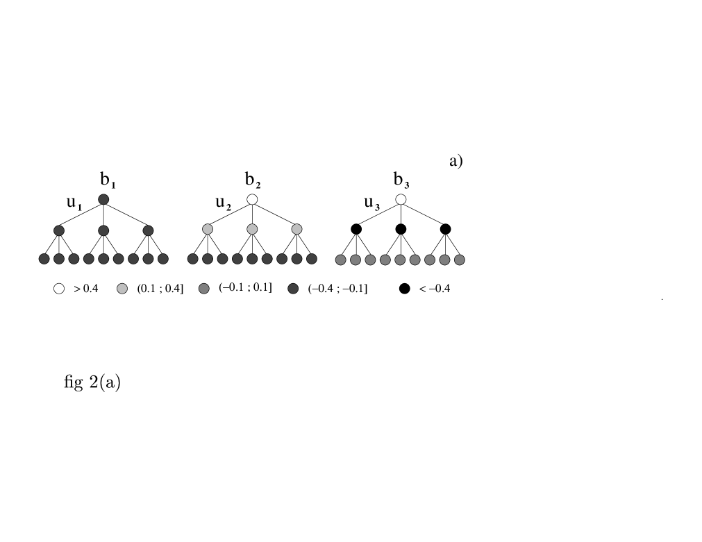
Figure 2(a) shows the three layered eigenvectors and their associated eigenvalues of the coupling matrix corresponding to a tree with and .
The set of eigenvalues arising from Eq. (7) may be ordered by decreasing value as . By Gershgorin’s theorem [12], the homogeneous eigenvector possesses the largest eigenvalue of , which is . On the other hand, for large the smallest eigenvalue is found to be
| (12) |
and similarly, we find
| (13) |
The eigenvalues appear in pairs and , as and above, according to the sign of the square root term. These pairs are related by
| (14) |
where
The eigenvalue arises whenever is odd, and it is not associated with another . Its value is
| (15) |
Thus, because of (14) and (15) the eigenvalues associated to the non-degenerate eigenvectors satisfy
| (16) |
Figure 3 shows the spectrum of eigenvalues , indicated by black dots, for a tree with ramification at successive depths . Eigenvalues associated to degenerate eigenvectors of , to be discussed next, are also shown in Fig. 3.
Degenerate eigenmodes
The subset of degenerate eigenvectors of the coupling matrix corresponding to a tree characterized by satisfy
| (17) |
where is the eigenvalue associated to a group of degenerate eigenvectors belonging to . The index goes from to and counts the different eigenvectors associated to the degenerate eigenvalue . The integer indices and label different eigenvalues .
The component of a vector corresponds to a cell of the tree labeled by the rule (5), i.e., . The eigenmodes are characterized by the following two properties,
| (18) |
that is, all the components of lying in successive levels vanish up to the level ; and
| (19) |
i.e., the sum of the components of an eigenvector , lying on the same level of the tree spatially described by , is zero.
An eigenvector is spatially uniform in part, having all its components, or equivalent cells, equal to zero up to level . The index counts the number of remaining non-vanishing layers in the eigenvector , and its possible values are . Each of the non-vanishing layers may be homogeneous, but different among each other. The index counts the number of possible different eigenvectors with different homogeneous, non-vanishing last layers. Thus, may take the values .
The index lifts the degeneracy of vectors with the same indices and . The remaining, non-vanishing last layers may in fact be non-homogeneous, and may consists of subtrees with homogeneous sub-levels, which would reproduce the structure of the layered non-degenerate eigenvectors . The level is the last vanishing layer in an eigenvector having non-vanishing layers. On this layer, there are components or cells, and each of these cells gives origin to layered subtrees, i.e., subtrees with homogeneous layers. These subtrees themselves are related by the sum property Eq. (19), which results in linearly independent subtrees. Therefore, the number of linearly independent eigenvectors with the same values and is . The index expresses the degeneracy of the eigenvectors associated to the eigenvalue , and it may take the values . In this way, the set of degenerate eigenvectors of the matrix corresponding to a tree is fully described.
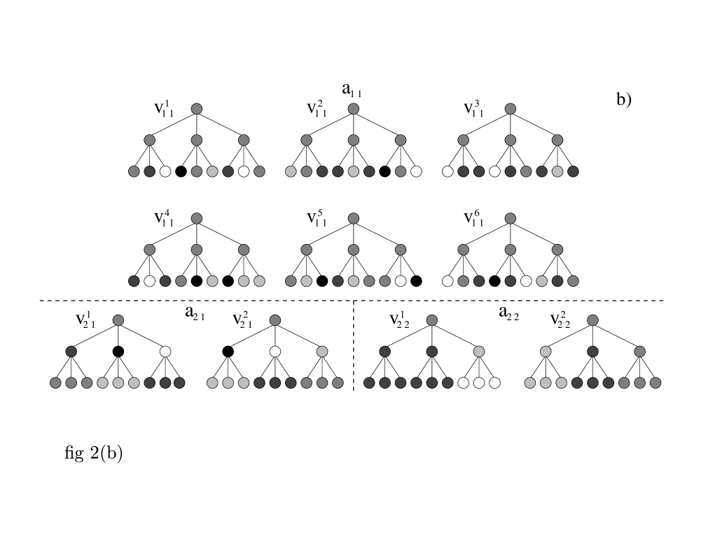
Figure 2(b) shows the subset of degenerate eigenvectors and the eigenvalues corresponding to a tree characterized by .
The index also expresses the form in which an eigenvalue arises in the spectrum of eigenvalues of . An eigenvalue appears for the first time at a level and stays in the spectrum of eigenvalues of at subsequent levels up to . Thus the index may take the values . On the other hand, different eigenvalues arise at the level of construction of the tree, which are counted by the index .
The total number of distinct eigenvalues of type belonging to the spectrum of a matrix associated to a tree is
| (20) |
Additionally, the eigenvalues that appear at a level satisfy the following property
| (21) |
and therefore the total sum of eigenvalues for a matrix associated to a tree will be,
| (22) |
Figure 3 shows the spectrum of eigenvalues for a tree with ramification at successive depths . Eigenvalues corresponding to non-degenerate eigenvectors are also shown there. Thus the distribution of the full spectrum of eigenvalues of the coupling matrix can be seen as a function of the depth of the tree in Fig. 3. Note that the full spectrum is always contained between the eigenvalues and .
The total number of distinct eigenvalues of , including both types and , and denoted by , is
| (23) |
Note that the total number of eigenvalues in the spectrum of is determined only by the depth of the tree and is independent of its ramification, although the specific values of the eigenvalues do depend on both and . Since there appear eigenvalues of type at each level and there are degenerate eigenvectors associated to each eigenvalue , the total number of independent eigenmodes in the subset is . In the non-degenerated subset there are independent eigenvectors, as we saw before. Therefore, the total number of independent eigenmodes of is
| (24) |
as expected.
Figure 4(a) shows the complete spectrum of eigenvalues of and the degeneracy fraction of each eigenvalue, for a tree characterized by parameters . The eigenvalues are indicated by dots and they are non-degenerate, while the degeneracy of each of the eigenvalues is plotted as a vertical bar. It is evident that both the distribution of eigenvalues and their degeneracies are nonuniform. Another convenient representation of the scaling properties of the spectrum of eigenvalues of the coupling matrix can be obtained by plotting the accumulated sum of the degeneracies of all eigenvalues, that is the measure of the spectrum of (denoted by ), on the eigenvalue axis for large , as in Fig. 4(b). The resulting graph presents the features of a devil s staircase, a fractal curve arising in a variety of nonlinear phenomena.
An example
As an example of calculation of eigenvectors, consider any tree with ramification and depth . The number of cells of the tree is . Thus, the tree consists of a mother cell at level connected to its daughters at level . The corresponding coupling matrix has the form
| (25) |
and the associated eigenvectors of have components. There exist two non-degenerate eigenvectors, which are the homogeneous , and , associated to the eigenvalues and , respectively. There is only the eigenvalue associated to degenerate eigenvectors . The total number of independent eigenmodes of is , and the total number of distinct eigenvalues is , in agreement with Eq.(23).
All the eigenvectors of have the level , with one component or cell; and the level , for which there are components. The layered eigenvector will have the form . Its eigenvalue equation , plus the normalization condition , yield the relations
| (26) |
whose solutions are , , . Thus,
| (27) |
On the other hand, the degenerate eigenmode has the form , satisfying properties (18) and (19), as well as the eigenvector equation and the normalization condition . These relations lead to
| (28) |
which imply that . Making and ; we get
| (29) |
with solutions, , . Thus
| (30) |
For the procedure can be repeated by making , , obtaining
| (31) |
In general, we get
| (32) |
giving eigenvectors in the degenerate subset for this example. With the addition of the two non-degenerate eigenvectors and , there are independent eigenvectors. Therefore, all the eigenvectors and eigenvalues associated to a matrix corresponding to a tree characterized by parameters are accounted for. Note that since the eigenvalue appears at level , it will stay in the spectrum of eigenvalues of for all subsequent levels of construction, i.e., arises for trees of any depth. Similarly, the eigenvalue and its associated homogeneous eigenvector always appear in a tree.
IV Bifurcation structure and stability of spatially synchronized states
Spatially synchronized states in extended systems are relevant since we are often interested in the mechanism by which a uniform system breaks its symmetry to form a spatial pattern as a parameter is changed. Consider spatially synchronized, period states such as , ; where , is a period orbit of the the local map, . The linear stability analysis of periodic, synchronized states in coupled map lattices is carried out by the diagonalization of in Eq. (4), and it leads to the conditions [13]
| (33) |
where is an eigenvalue, in either set or , of the coupling matrix describing a tree . There are different values of (Eq. (23)) to be used in Eqs. (33).
The nonuniform distribution of the eigenvalue spectrum is manifested in the stability of the synchronized states through this relation and give rise to important differences when compared, for instance, with the bifurcation structure on regular lattices. As an application, consider a local dynamics described by the logistic map, . In this case, the bifurcation conditions, Eq. (33), for the period , synchronized state on a tree characterized by parameters can be expressed as the set of curves
| (34) |
For each sign, Eqs. (34) yield boundary curves in the plane which determine the stability regions of the period , synchronized states on the tree.
The scaling structure for the period-, synchronized states in trees is similar to that of a any lattice described by a diffusive coupling matrix, since the form of Eq. (34) is the same in any case. As for any lattice (for example regular Euclidean lattices [13] or fractal lattices [1]), the stability regions for the period-, synchronized states in the plane scale as , and , where and are Feigenbaum’s scaling constants for the period doubling transition to chaos. However, the specific structure of the eigenvalue spectrum of the coupling matrix determines the shapes and gaps of the regions of stability of synchronized, periodic states.
The boundary curves Eqs. (34) for the synchronized, fixed point state are given by the straight lines
| (35) |
which are first crossed for the most negative eigenvalue, . Fig. 5(a) shows the boundary curves Eq. (34) in the plane for the period-two (), synchronized state on a tree with , which are given by the two sets
| (36) |
and
| (37) | |||||
| (38) |
The boundary between the synchronized, fixed point state and the synchronized period-two state is at . The upper boundaries (corresponding to in the r.h.s of Eqs. (36)-(37)) have minima at values and (for any period , depends on ). Fig. 5(b) shows a magnification of Fig. 5(a) around the minima of the upper boundaries. The distribution of the minima and the presence of nonuniformly distributed gaps (niches) in the boundary curves reflect the nonuniform structure of the eigenvalue spectrum. Since the nonuniformity in the distribution of eigenvalues persists at any depth of a tree, this property allows for regions of stability of the synchronized states (niches) characteristic of trees and which are not present in other geometries, for example in regular lattices, where the distribution of eigenvalues of the coupling matrix is uniform and continuous in the limit of infinite size lattices.
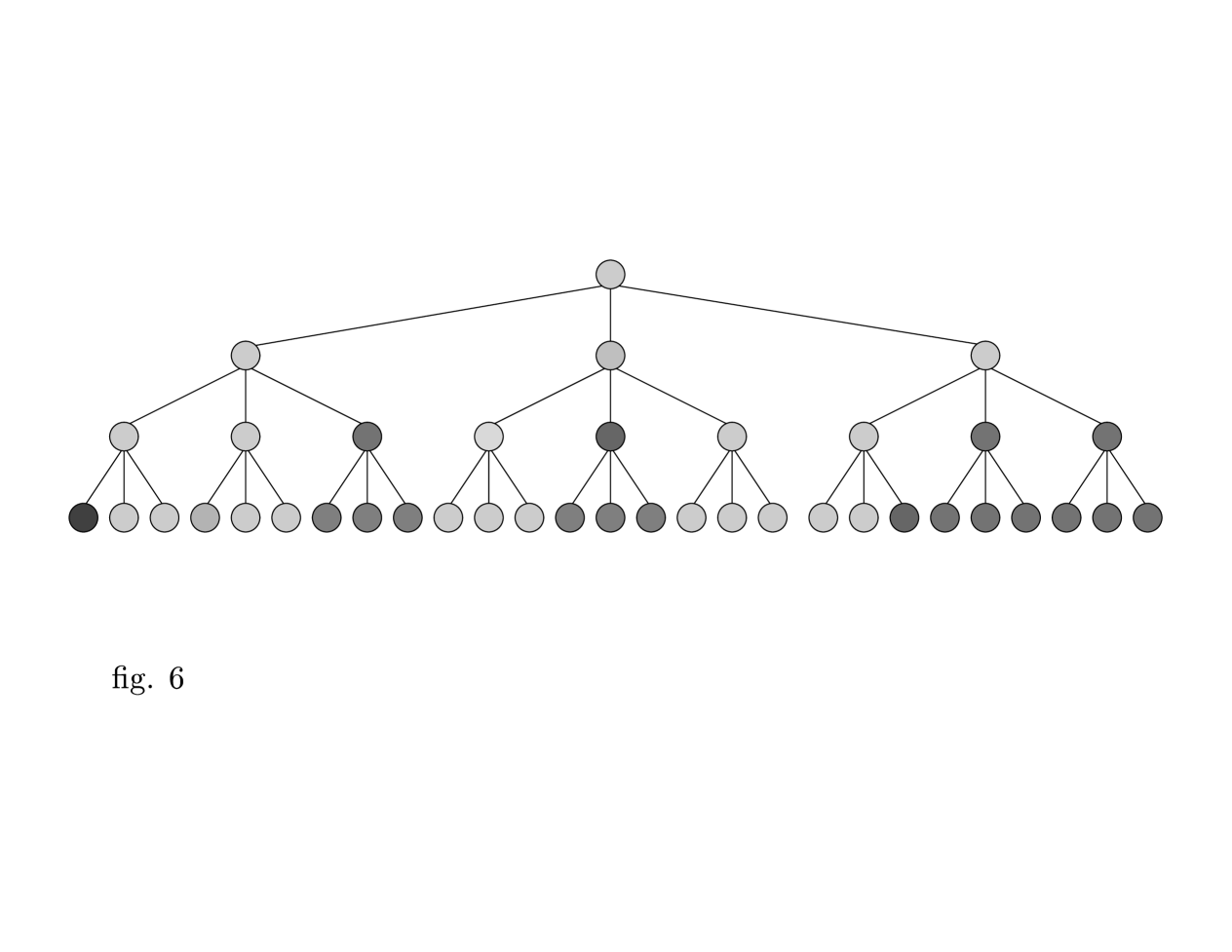
The set of eigenvectors of the coupling matrix constitute a complete basis (normal modes) on which a state of the system can be represented as a linear combination of these vectors. The evolution of then reflects the stabilities of the normal modes. Fig. 5(b) shows how the synchronized state may become unstable through crossing of the upper boundary; the first boundary segment crossed determines the character of the instability. For example, consider an initial state consisting of a small perturbation of the synchronized, period- state at parameter values just beyond the boundary segment corresponding to indicated by a cross in Fig. 5(b), where this initial state is unstable. The inhomogeneous period- final spatial pattern is represented in Fig. 6; it corresponds to a linear combination of the six eigenmodes and associated to the degenerate eigenvalue of the matrix corresponding to the tree . All other modes are unstable in this region of parameter space. For any depth of the tree, and any period , the boundary curve separates a niche of the synchronized state from the stable region for the eigenmodes corresponding to . Thus, a transition between these two spatial patterns can always be observed in the appropriate regions of the plane.
V Conclusions
In a system of interacting agents, such as the models presented in this article, the coupling matrix contains the connectivity of the network and it determines the spatial patterns that can arise in the system. The underlying inhomogeneous structure of trees has pronounced effects on the spatial patterns that can be formed by reaction-diffusion processes on these lattices. The spatial patterns are determined by the eigenvectors of the coupling matrix ; and the stability of the synchronized states is determined by the corresponding eigenvalues. The set of normal modes of the coupling matrix reflect the connectivity of the tree. These modes have complex spatial forms but they are analogous to the Fourier eigenmodes arising in regular Euclidean lattices. On the other hand, the distribution of eigenvalues of and their degeneracies are nonuniform. These features affect the bifurcation properties of dynamical systems such as coupled map defined on trees. The scaling structure of the synchronized, period-doubled states is similar for both uniform and hierarchical lattices, but the nature of the bifurcation boundaries is different. For trees, the boundary curves are determined by the spectrum of eigenvalues of the coupling matrix, which has a nonuniform density. The nonuniform distribution of eigenvalues leads to gaps or niches in the boundary curves that are not present for coupled maps on uniform lattices, where the spectrum of eigenvalues is continuous.
We have examined only the simplest spatiotemporal patterns that can be formed on treelike geometries; however, the formalism presented in Sec. II can be applied to many other processes, such as nontrivial collective behavior, excitation waves, phase transitions, domain segregation and growth on trees. The formalism is also useful for continuous-time local dynamics. Similarly, extensions of this work are possible in order to include networks with variable ramification and/or depths.
The study of dynamical systems defined on trees and other nonuniform substrates should allow us to gain insight into previously unexplored spatiotemporal phenomena on inhomogeneous systems and to understand better the relationship between topology and collective properties of networks.
Acknowledgment
This work was supported by the Consejo de Desarrollo Científico, Humanístico y Tecnológico of the Universidad de Los Andes, Mérida, Venezuela.
REFERENCES
- [1] M. G. Cosenza and R. Kapral, Phys. Rev. A 46, 1850 (1992).
- [2] M. G. Cosenza and R. Kapral, Chaos 4, 99 (1994).
- [3] D. J. Watts and S. H. Strogatz, Nature 393, 440 (1998).
- [4] P. M. Gade, H. A. Cerdeira, and R. Ramaswamy Phys. Rev. E 52, 2478 (1995).
- [5] S. Sinha, G. Perez, and H. A. Cerdeira, Phys. Rev. E 57, 5217 (1998).
- [6] P. M. Gade, Phys. Rev. E 54, 64 (1996).
- [7] D. Avnir The fractal approach to heterogeneous Chemistry, New York, Wiley (1989).
- [8] C. Meneveau and K. R. Sreenivasan, Phys. Rev. Lett. 59, 1424 (1987).
- [9] T. Hogg, B. A Huberman and J. McGlade, Proc. R. Soc. London B 237, 43 (1989).
- [10] P. Houlahan and J. Scalo, Ap. J. 393, 172 (1992).
- [11] D. Amit, Modelling Brain Function: The World of Attractor Neural Nets, Cambridge U. Press, Cambridge, 1989.
- [12] See for example, S. Barnett, Matrices, Methods and Applications, Oxford University Press, Oxford (1990).
- [13] I. Waller and R. Kapral, Phys. Rev. A 30, 2047 (1984).