Exact and semiclassical Husimi distributions of Quantum Map Eigenstates

Abstract

The projector onto single quantum map eigenstates is written only in terms of powers of the evolution operator, up to half the Heisenberg time, and its traces. These powers are semiclassically approximated, by a complex generating function, giving the Husimi distribution of the eigenstates. The results are tested on the Cat and Baker maps.

I Introduction

The relation between the classical invariant structures of a dynamical system and its quantum counterparts, the eigenenergies and eigenstates, is not completely understood and is an intense subject of investigation. When the system is integrable the eigenenergies are determined by the well-known Bohr-Sommerfeld or EBK quantization rules and the eigenfunctions have a very intuitive phase space structure: they are essentially localized on the quantized tori and they present characteristic quantum features –interference fringes for the Wigner function [1] or zeros for the Husimi function [2]– away from them. No such clear picture is available for the eigenstates of chaotic systems and much work [3, 4, 5, 6] has gone into trying to disentangle the purely statistical aspects of the eigenfunctions from the specific dynamical features such as scars and localization.

Although a lot of recent work deals with the study of the statistical aspects of chaotic wavefunctions [7] we concentrate here on the purely dynamical aspects and explore how well the semiclassical formulae can reproduce the details of individual eigenfunctions.

With regards to spectral properties the theoretical tool for this analysis is the Gutzwiller trace formula [8] relating the spectral density to the periodic orbits. As is well known, this relationship is fraught with uncertainties both due to the approximations involved, as to the fact that it diverges where it is supposed to locate the single eigenenergies and to the sheer complexity of adding the contributions of an exponentially increasing number of periodic orbits. Some of these difficulties can be overcome by resummation techniques [9] that limit the exponential increase by partially restoring the unitarity of the propagator, lost in the semiclassical approximation.

In the present work we extend these resummation methods to the calculation of eigenfunctions of chaotic maps. We utilize Fredholm theory to construct a projector on single eigenstates whose expression is directly amenable to semiclassical approximations. These approximations share the same advantages - and the drawbacks- of the resummation techniques available for spectral properties.

In section 2 we construct explicitly the projector on single eigenstates. This is achieved exactly in terms of a finite sum on powers of the quantum map propagator and its traces. The cut-off time is half the Heisenberg time due to the explicit imposition of unitarity. In section 3 these formulae are implemented semiclassically by a) approximating the traces in terms of actions and instabilities of periodic orbits in the usual way, and b) by computing the propagator in the coherent state representation in terms of specially devised complex generating functions.

The final result is a semiclassical expression for the Husimi function of an eigenstate in terms of properties of a finite set of periodic orbits.

In section 4 we apply the method to the cat map –where the semiclassical approximation is exact – and to the baker map where we can test the approximation.

The formulae are here applied as a test to simple maps, but they can be easily adapted to more realistic Hamiltonian systems by selecting an appropriate Poincaré section [11].

II Projector on single eigenstates

For a map, the density of Floquet states can be expressed in the usual way in terms of traces by the formula

$$d(\epsilon)=\frac{2\pi}{N}+\sum_{n=1}^{\infty}[tr\hat{U}^{n}e^{-i\epsilon n}]+C.C.$$ (1)

$1/N$ plays the role of Plank’s constant $h$, $n$ is the discrete time, and $\hat{U}$ is the unitary quantization of the map. The density of states results in a $2\pi$ periodic function with unit $\delta$-spikes at the eigenangles $\epsilon_{k}$, defined by

$$\hat{U}|\psi_{k}\rangle=e^{i\epsilon_{k}}|\psi_{k}\rangle\ .$$ (2)

Semiclassical approximations using this formula require the calculation of traces of powers of the map for large values of $n$ which are in turn related to classical orbits of the map by the Gutzwiller-Tabor [8] trace formula

$$b_{n}=tr\hat{U}^{n}\approx\sum_{\gamma}A_{\gamma}\exp\left[i(S_{\gamma}/\hbar-\mu_{\gamma}\pi/2)\right]\ ,$$ (3)

where $\gamma$ label the $n$-periodic orbits of the map, $S_{\gamma}$ is the action, $\mu_{\gamma}$ is the Maslov index, and $A_{\gamma}$ is a coefficient related to the monodromy matrix. The approximation is valid for fixed $n$ in the limit as $N\rightarrow\infty$ (but not vice-versa).

A more efficient scheme starts from the spectral determinant

$$P(s)=\det(\hat{I}-s\hat{U})$$ (4)

which vanishes at $s=s_{k}=e^{-i\epsilon_{k}}$ and which can be expanded as

$$P(s)=\sum_{n=0}^{N}\beta_{n}s^{n}\ .$$ (5)

The coefficients $\beta_{n}$ can be computed recursively from the traces as

$$\beta_{n}=-\frac{1}{n}\sum_{j=1}^{n}\beta_{n-j}b_{j}$$ (6)

and therefore when computed semiclassically as in (3) they are expressed in terms of linear combinations of periodic orbits (pseudo orbits [12]) of period up to $n$.

The advantage over the calculation in term of traces is that only $N$ coefficients need to be calculated. Moreover as a consequence of unitarity the symmetry

$$\beta_{N-j}=(-1)^{N}\det\hat{U}~{}\bar{\beta}_{j}$$ (7)

can be imposed, so that only $N/2$ coefficients are needed and therefore only periodic trajectories for times up to $N/2$ (i.e. half the Heisenberg time) are involved for a semiclassical calculation. This is now an optimal encoding of the eigenvalues in terms of traces, with the $N$ real phases $\epsilon_{k}$ expressed exactly in terms of the $N/2$ complex coefficients $\beta_{n}$

It is convenient to define another function [13], proportional to the spectral determinant, which has the same roots. Utilizing the symmetry (7), for an even $N$, this function can be written

$$Z(s)=\frac{P(s)}{\beta_{N/2}~{}s^{N/2}}=1+\frac{1}{\beta_{N/2}}\sum_{n=0}^{N/2-1}\beta_{n}~{}s^{n-N/2}+\frac{1}{\bar{\beta}_{N/2}}\sum_{n=0}^{N/2-1}\bar{\beta}_{n}~{}s^{N/2-n}\ .$$ (8)

When $s$ is on the unit circle $1/s=\bar{s}$, and then the second sum is the complex conjugate of the first. Then the function $Z(s)$ becomes real on $|s|=1$.

Unitarity also implies that the spectral determinant has all its zeros on the unit circle. However when the coefficients are computed semiclassically this is no longer guaranteed. If the symmetry (7) is imposed the resulting spectral determinant becomes self-inversive, which is a necessary -but by no means sufficient- condition for unitarity [14]. Self-inversive polynomials have the following properties [15]:

1) All zeros are either on the unit circle or symmetric with respect to it. Thus as a function of a continuous parameter the zeros of a self-inversive polynomial can only leave the unit circle in pairs by degenerating on it.

2) If $P(s)$ has only single roots then $dP/ds$ has no zeros on the unit circle.

A Green Operator

Very similar techniques can be implemented for the calculation of matrix elements and therefore of eigenfunctions. To obtain the eigenfunctions of the unitary matrix $\hat{U}$, we define a Green operator

$$\hat{G}(s)=\frac{f(\hat{U})}{\hat{I}-s\hat{U}}\ ,$$ (9)

which, as an analytic function of $s$, has poles at $s=s_{k}=e^{-i\epsilon_{k}}$, and the residues are proportional to the projectors $\hat{P}_{k}=|\psi_{k}\rangle\langle\psi_{k}|$. To obtain normalized projectors, we instead define a normalized Green operator

$$\hat{g}(s)=\frac{\hat{G}(s)}{tr[\hat{G}(s)]}\ .$$ (10)

At the poles, the singularities cancel and we obtain $\hat{g}(s_{k})=\hat{P}_{k}$. $f(\hat{U})$ is left arbitrary for the moment, and specific choices -made below- will be used to obtain formulae with different properties.

We can expand the preceding expression utilizing the transpose cofactor matrix to write the Green operator

$$\hat{g}(s)=\frac{f(\hat{U})~{}C^{t}(\hat{I}-s\hat{U})}{tr[f(\hat{U})~{}C^{t}(\hat{I}-s\hat{U})]}\ .$$ (11)

The transpose cofactor matrix can be written as a finite power series in $s$

$$C^{t}(\hat{I}-s\hat{U}) = \sum_{n=0}^{N-1}s^{n}\hat{X}_{n}\ ,$$ (12)

$$\hat{X}_{n} = \sum_{i=0}^{n}\beta_{i}~{}\hat{U}^{n-i}\ .$$ (13)

By the unitarity of $\hat{U}$, the $\hat{X}_{n}$ matrices satisfy the following symmetry

$$\hat{X}_{N-j}=-\hat{U}^{\dagger}(-1)^{N}\det\hat{U}~{}\hat{X}_{j-1}^{\dagger}\ .$$ (14)

Utilizing this symmetry two choices of $f(\hat{U})$ lead to expansions with useful properties:

a) For $f(\hat{U})=\hat{U}$, for even $N$, the corresponding Green function is

$$\hat{g}_{a}(s)=\frac{\sum_{n=0}^{N/2-1}s^{n}~{}\hat{U}\hat{X}_{n}-\det\hat{U}~{}s^{N-1}\sum_{n=0}^{N/2-1}s^{-n}~{}\hat{X}^{\dagger}_{n}}{\sum_{n=0}^{N/2-1}s^{n}~{}tr\left(\hat{U}\hat{X}_{n}\right)-\det\hat{U}~{}s^{N-1}\sum_{n=0}^{N/2-1}s^{-n}~{}tr\left(\hat{X}^{\dagger}_{n}\right)}\ .$$ (15)

Replacing the expansion of the $\hat{X}_{n}$ operators in powers of $\hat{U}$, we obtain

$$\hat{g}_{a}(s)=\frac{\sum_{i=0}^{N/2-1}c_{i}(s)~{}\hat{U}^{i+1}-\det\hat{U}~{}s^{N-1}\sum_{i=0}^{N/2-1}\bar{c_{i}}(1/\bar{s})~{}\hat{U}^{\dagger~{}i}}{\sum_{i=0}^{N/2-1}c_{i}(s)~{}tr\left(\hat{U}^{i+1}\right)-\det\hat{U}~{}s^{N-1}\sum_{i=0}^{N/2-1}\bar{c_{i}}(1/\bar{s})~{}tr\left(\hat{U}^{\dagger~{}i}\right)}\ ,$$ (16)

in which the projector is expressed as a finite combination of the first $N/2$ powers of the propagator.

The coefficients $c_{i}$ are obtained from the $\beta_{n}$

$$c_{i}(s)=\sum_{n=i}^{N/2-1}\beta_{n-i}~{}s^{n}\ .$$ (17)

This normalized Green operator has no singularities as $s$ goes around on the unit circle. This can be demonstrated because the denominator is equal to $-dP/ds$ (see Appendix A). Then by the second property of the self-inversive polynomials it is guaranteed that this denominator never takes the zero value for $s$ over the unit circle. This property, guaranteed by unitarity, will remain true –even when the traces and propagator are calculated semiclassically– as long as self inversiveness is maintained.

b) For $f(\hat{U})=\hat{I}+s\hat{U}$ , $\hat{G}(s)$ in (9) is the Cayley transform of $\hat{U}$ and is therefore hermitian on the unit circle. In this case

$$\hat{g}_{b}(s)=\frac{\sum_{n=0}^{N}s^{n}~{}\hat{Y}_{n}}{\sum_{n=0}^{N}s^{n}~{}tr\left(\hat{Y}_{n}\right)}$$ (18)

with

$$\hat{Y}_{n}=\hat{X}_{n}+\hat{U}\hat{X}_{n-1}=2\hat{X}_{n}-\beta_{n}\hat{I}\ .$$ (19)

These new operators satisfy a simpler symmetry relation than the preceding $\hat{X}_{n}$, analogous to the symmetry of the $\beta_{n}$ coefficients

$$\hat{Y}_{N-j}=-(-1)^{N}\det\hat{U}~{}\hat{Y}^{\dagger}_{j}\ .$$ (20)

In this case, for even $N$, the normalized Green operator can be written as

$$\hat{g}_{b}(s)=\frac{\hat{\Sigma}(s)-\hat{\Sigma}^{\dagger}(1/\bar{s})}{tr\left[\hat{\Sigma}(s)\right]-tr\left[\hat{\Sigma}^{\dagger}(1/\bar{s})\right]}\ ,$$ (21)

where

$$\hat{\Sigma}(s)=\frac{1}{\beta_{N/2}}\left[\frac{1}{2}\hat{Y}_{N/2}+\sum_{n=0}^{N/2-1}s^{n-N/2}~{}\hat{Y}_{n}\right]\ .$$ (22)

In this expression, more symmetrical than (16), the numerator is anti-hermitian on the unit circle, and the denominator is purely imaginary. The basic operator $\hat{\Sigma}(s)$ is a Fourier transform of the $\hat{Y}_{n}$ operators and their traces. When utilizing this finite representation, they then become the basic objects of study in the time domain, in place of the propagator and its traces.

When $\hat{U}$ is a finite matrix, $\hat{g}_{a}(s)$ and $\hat{g}_{b}(s)$ are both rational analytic functions of $s$. They are identical at the eigenvalues $s=s_{k}$ (on the unit circle). However their zero and singularity structure is quite different.

In particular $\hat{g}_{a}(s)$, as noted, has a denominator which does not vanish on the unit circle, even when the coefficients are computed approximately, as long as self-inversiveness is imposed on them. The operator $\hat{g}_{a}(s)$ then, has no singularities in a small strip enclosing the unit circle and can be followed continuously from eigenvalue to eigenvalue. A disadvantage is that $\hat{g}_{a}(s)$ is not hermitian (except at the values $s=s_{k}$). On the contrary $\hat{g}_{b}(s)$ is hermitian on the unit circle, but its singularities (the zeroes of the denominator) are precisely on the unit circle, in between two successive eigenvalues.

It should be noticed that, although for simplicity all the above formulae are written for even $N$, they are easily adapted to the odd case, with minimal changes.

The preceding operator expressions for $\hat{g}_{a}(s)$ and $\hat{g}_{b}(s)$ provide a common structure that underlies all further semiclassical approximations. Depending on the representation used to evaluate them, they can yield results for transition probabilities, phase space distributions, response functions or wave function correlations. This is achieved by linking the spectral properties of the map to a finite number of traces and matrix elements of the propagator. To apply them one needs the semiclassical evaluation of the propagator traces as in (3)- which are representation independent- and also of the semiclassical propagator in the chosen representation. For example if they are computed in the coordinate representation they provide expressions for $|\langle x|\psi_{k}\rangle|^{2}$. If the propagator is computed in the Weyl representation [17] they yield the Wigner distribution of eigenfunctions [18]. In all cases the unitarity of the propagator - which is generally only approximate in semiclassical treatments - is partially restored by the imposition of the symmetries (7,14,20). In the next section the above formalism is developed in the coherent state representation to obtain expressions for semiclassical Husimi distributions.

III Semiclassical approximation in the coherent state representation

The formulae derived in the previous section are exact and for maps can, at first sight, seem just a complicated way of looking at a simple algebraic eigenvalue problem. However, they are prepared in such a way as to make the semiclassical transition as clear as possible and to unveil the necessary approximations involved in such a transition,

The coherent state mean value of $\hat{g}(s)$ is

$${\cal H}(s,z,\bar{z})\equiv\frac{\langle z|\hat{g}(s)|z\rangle}{\langle z|z\rangle}\ .$$ (23)

This is a phase space distribution, analytic in $s$, which becomes the Husimi distribution of the eigenstates $|\psi_{k}\rangle$ at the values $s_{k}=e^{-i\epsilon_{k}}$.

Its properties, reflecting the zeroes and singularities of $\hat{g}(s)$ can be followed continuously in the $s$ complex plane. Its calculation involves the $N/2$ coherent state return amplitudes

$$C_{n}(z,\bar{z})\equiv\frac{\langle z|\hat{U}^{n}|z\rangle}{\langle z|z\rangle}$$ (24)

in addition of the $N/2$ traces

$$b_{n}=tr\hat{U}^{n}=\int dz~{}d\bar{z}~{}C_{n}(z,\bar{z})\ .$$ (25)

The first admits immediately a well known semiclassical approximation in the time domain, namely the Gutzwiller-Tabor trace formula (3). The stationary phase approximations involved in the derivation are of course valid for fixed time $n$ and for $\hbar\rightarrow 0$, or equivalently, $N\rightarrow\infty$, and their use in the regime $n\approx N/2$ needed for the exact calculation is questionable.

The semiclassical calculation of the return amplitudes $C_{n}(z,\bar{z})$ can be done by stationary phase calculation of the integral

$$\langle z_{f}|\hat{U}^{n}|z_{i}\rangle=\int\int\langle z_{f}|q_{f}\rangle\langle q_{f}|\hat{U}^{n}|q_{i}\rangle\langle q_{i}|z_{i}\rangle~{}dq_{i}~{}dq_{f}\ ,$$ (26)

where

$$\langle z|q\rangle=\frac{\exp\left\{-\frac{1}{2\hbar}\left[z^{2}+q^{2}-2\sqrt{2}zq\right]\right\}}{\sqrt[4]{\pi\hbar}}$$ (27)

is the coherent state in coordinate representation, and the propagator has the usual Van Vleck form

$$\langle q_{f}|\hat{U}^{n}|q_{i}\rangle=\frac{1}{\sqrt{2\pi i\hbar}}\sum_{\gamma}\sqrt{\frac{\partial^{2}S^{(n)}_{\gamma}(q_{i},q_{f})}{\partial q_{i}\partial q_{f}}}~{}\exp\left[~{}\frac{i}{\hbar}S^{(n)}_{\gamma}(q_{i},q_{f})\right]\ .$$ (28)

The sum must be made over all the paths in the phase space of the corresponding classical map that connect $q_{i}$ with $q_{f}$ in $n$ steps. Additional phases connecting the different branches, the Maslov indices, must be added to $S^{(n)}_{\gamma}$.

The calculation of the integral (26) with the Van Vleck approximation (28) can be done as usual by stationary phase and the result has the structure of another Van Vleck formula with complex coordinates for a generating function.

$$\langle z_{f}|\hat{U}^{n}|z_{i}\rangle=\sum\sqrt{-i\frac{\partial^{2}G_{3}}{\partial\bar{z}_{i}\partial z_{f}}}~{}\exp\left[-\frac{i}{\hbar}G_{3}(\bar{z}_{i},z_{f})\right]\ .$$ (29)

This new classical generating function is a complex Legendre transform of the action $S$

$$G_{3}=-S+\frac{1}{2}(p_{f}q_{f}-p_{i}q_{i})+\frac{i}{4}(q_{f}^{2}+p_{f}^{2}+q_{i}^{2}+p_{i}^{2})\ ,$$ (30)

or equivalently, in the complex coordinates

$$z = \frac{1}{\sqrt{2}}\left(q-ip\right)$$ (31)

$$\bar{z} = \frac{1}{\sqrt{2}}\left(q+ip\right)\ ,$$ (32)

it can be written as

$$G_{3}=-S+\frac{i}{4}\left(z_{f}^{2}+2z_{f}\bar{z}_{f}-\bar{z}_{f}^{2}\right)-\frac{i}{4}\left(z_{i}^{2}-2z_{i}\bar{z}_{i}-\bar{z}_{i}^{2}\right)\ .$$ (33)

This function depends explicitly on $\bar{z}_{i},z_{f}$ variables, and yields the equations of motion

$$z_{i}=-i\frac{\partial G_{3}}{\partial\bar{z}_{i}}\ ,~{}~{}~{}~{}~{}~{}~{}~{}~{}\bar{z}_{f}=-i\frac{\partial G_{3}}{\partial z_{f}}\ .$$ (34)

These are algebraic equations that define the map implicitly provided $\frac{\partial^{2}G_{3}}{\partial\bar{z}_{i}\partial z_{f}}\neq 0$ where the sum must be made over complex paths that connect the point $\bar{z}_{i}$ to $z_{f}$. These formulae show that the return amplitude $C_{n}$ has as exponent the function $G_{3}(\bar{z},z)-i\bar{z}z$ which using (34) can be shown to be stationary at the periodic points. Quadratic approximation of the generating function at these points yields the coherent state return amplitudes as a sum of Gaussian peaks centered on them

$$C_{n}(z,\bar{z})=\sum_{\gamma}\frac{1}{\sqrt{u_{\gamma}}}\exp\left[-\frac{1}{\hbar}{\cal G}^{\gamma}(z,\bar{z})+\frac{i}{\hbar}S_{\gamma}\right]\ .$$ (35)

$${\cal G}^{\gamma}(z,\bar{z})=\frac{1}{u_{\gamma}}\left[\frac{\bar{v}_{\gamma}}{2}(\bar{z}-\bar{z}_{\gamma})^{2}+(u_{\gamma}-1)(\bar{z}-\bar{z}_{\gamma})(z-z_{\gamma})-\frac{v_{\gamma}}{2}(z-z_{\gamma})^{2}\right]\ ,$$ (36)

where $z_{\gamma},\bar{z}_{\gamma}$ are the position of the periodic points, $S_{\gamma}$ are the corresponding actions, and $u_{\gamma},v_{\gamma}$ and $\bar{v}_{\gamma}$ are the elements of the complex monodromy matrix defined by

$$\left(\begin{array}[]{cc}\partial z_{f}/\partial z_{i}&\partial z_{f}/\partial\bar{z}_{i}\\ \partial\bar{z}_{f}/\partial z_{i}&\partial\bar{z}_{f}/\partial\bar{z}_{i}\end{array}\right)=\left(\begin{array}[]{cc}u&\bar{v}\\ v&\bar{u}\end{array}\right)$$ (37)

calculated on the corresponding periodic point.

Using (35) for the return amplitudes and (3) for the traces, the Husimi distributions of eigenstates are explicitly written in terms of properties of periodic points of all periods up to half the Heisenberg time $N/2$.

Although the semiclassical approximations are available in the time domain for the traces $b_{n}$ and the return amplitudes $C_{n}(z,\bar{z})$ it is clear from our formulae that the essential ingredients for the calculations are the coefficients $\beta_{n}$ and the operators $\hat{X}_{n}$ (or $\hat{Y}_{n}$). These are related by (6) and (13) to $b_{n}$ and $C_{n}$ and therefore can be recursively computed from them. This procedure yields the $\beta_{n}$ as linear combinations of products –the so called pseudo-orbits– of terms involving many periodic orbits of different periods and with signs implying many possible cancellations between long and short orbits. The same situation prevails for the $\hat{X}_{n}$ (or $\hat{Y}_{n}$). The expressions yield linear combinations of return amplitudes at many different times. In fact $\hat{X}_{n}(z,\bar{z})$ give the phase space distribution of pseudo-orbits and it is easy to show that $\beta_{n}=(N-n)~{}tr\hat{X}_{n}$. In view of the cancellations involved it would be very desirable to have a direct semiclassical derivation –both for $\beta_{n}$ and $\hat{X}_{n}$– that would not go through the indirect procedure of approximating $b_{n}$ and $\hat{U}_{n}$, and then recursively computing $\beta_{n}$ and $\hat{X}_{n}$. However to our knowledge such a derivation is not available.

IV Numerical calculations

We will test the methods proposed on two simple well known maps: the cat map, and the baker map.

For the cat map

$$\left(\begin{array}[]{c}q_{f}\\ p_{f}\end{array}\right)=\left(\begin{array}[]{cc}a&b\\ c&d\end{array}\right)\left(\begin{array}[]{c}q_{i}\\ p_{i}\end{array}\right)(mod~{}1)$$ (44)

with $a,b,c$ and $d$ integer numbers, and $ad-bc=1$, the Van Vleck formula in the $q_{i},q_{f}$ representation is exact [19] and the corresponding one in the coherent state representation can be computed explicitly.

The transformation to complex coordinates leads to the map

$$\left(\begin{array}[]{c}z_{f}\\ \bar{z}_{f}\end{array}\right)=\left(\begin{array}[]{cc}u&\bar{v}\\ v&\bar{u}\end{array}\right)\left(\begin{array}[]{c}z_{i}\\ \bar{z}_{i}\end{array}\right)$$ (51)

with

$$u = \frac{1}{2}\left[(a+d)+i(b-c)\right]\ ,$$ (52)

$$v = \frac{1}{2}\left[(a-d)+i(b+c)\right]\ .$$ (53)

and its quantization with (28) is obtained exactly by Gaussian integration. The coherent state return amplitudes are computed with the formulae (35) and (36), with the advantage that the coefficients of the monodromy matrix are the same for all the periodic points of a given period. Since the cat map is defined on the torus we use periodized coherent states [2]. With this result we can test our formulae keeping in mind that for this special case the semiclassical approximation is exact.

In Fig.1 we first look at quantities in the time domain, i.e. as a function of $n$. The correlations $|C_{n}(z,\bar{z})|^{2}$ display for short times Gaussian peaks at the n-periodic points.

However we have seen that the irreducible information about eigenstates is carried by more complicated operators such as the $\hat{X}_{n}$ in (13) or the $\hat{Y}_{n}$ in (19). These operators carry the phase space information that corresponds to the pseudo-orbits in the resummation of trace formula. In fact many different powers of $\hat{U}$ contribute to them and give rise to complex interference structures in phase space. The pseudo-orbit contributions –contained in the coefficient $\beta_{n}$– are obtained from the fact that $\beta_{n}=(N-n)~{}tr\hat{X}_{n}$.

In Fig.2 we have displayed the first few operators $\hat{U}\hat{X}_{n}$ appearing in the expansion of $g_{a}(s)$. For very short times we notice the simple superposition of the patterns of $C_{n}(z,\bar{z})$. In particular $\hat{U}\hat{X}_{2}$ shows peaks at the period 1, period 2 and period 3 periodic orbits. For longer times ($\hat{U}\hat{X}_{3}$) the interferences between orbits of different periods are very strong and one can barely notice the period 4 orbits, while the dominant structure is of period 1. This is in striking contrast with the regular appearance of periodic points in the return amplitudes. Notice also the totally unexpected –and for us unexplained– appearance of a strong periodicity (of period three) in the phase space patterns, which is totally invisible in the $C_{n}$ coefficients. We cannot give an explanation to this behavior except noting that a direct semiclassical calculation of these coefficients would be very desirable and might be more effective than one which goes through the calculation with periodic points.

The smooth dependence of the operator $\hat{g}(s)$ on the quasi energy variable allow us to consider the exact response function as a distribution in phase space depending continuously on $s$, thus allowing an exact interpolation for all values of $s$. The Husimi eigen-distributions are particular values of this function which should be positive and display a pattern of $N$ zero values, in accordance with the general properties of Husimi distributions of pure states on the torus. [2]

We display in Fig.3 the real part of ${\cal H}_{a}(e^{-i\epsilon},z,\bar{z})$ for values of $\epsilon$ near an eigenvalue. The distribution shows a very stable pattern of minima that gradually develops into $N=14$ zeros at $\nu=\epsilon/2\pi=0.4167$. At this point $Z(e^{-i\epsilon})=0$, the distribution is positive and we verify that the imaginary part vanishes for every phase space point. This is the signal [2] that a true projector has been reached and that the Husimi distribution is the modulus of an analytic function with $N$ zeros. Past the eigenvalue the distribution can become negative but the pattern of minima remains very stable. At the values where $Z(e^{-i\epsilon})$ has an extremum, in between zeros, we show in the appendix that the distribution becomes flat with value $1/N$. At this point the pattern of minima changes and picks up the structure of zeros of the next eigenfunction.

For cat maps the semiclassical formulae are exact and therefore the above results merely confirm that the whole scheme is consistent and accurate but they do not really test the semiclassical approximation. Towards this purpose we consider another simple linear map –the baker’s– where the semiclassics is not exact. The classical $T$-iteration of the baker map from the $(q_{0},p_{0})$ to $(q_{T},p_{T})$ real coordinates [20], takes the complex form

$$z_{T} = u_{T}~{}z_{0}+v_{T}~{}\bar{z_{0}}-w_{T}$$ (54)

$$\bar{z}_{T} = v_{T}~{}z_{0}+u_{T}~{}\bar{z_{0}}-\bar{w}_{T}$$ (55)

$$u_{T} = \frac{2^{T}+2^{-T}}{2}=\cosh(T\ln 2)$$ (56)

$$v_{T} = \frac{2^{T}-2^{-T}}{2}=\sinh(T\ln 2)$$ (57)

$$w_{T} = \frac{1}{\sqrt{2}}\left(\gamma+i~{}2^{-T}\gamma^{\dagger}\right)$$ (58)

$\gamma$ is the integer part of $2^{T}q_{0}$ and $\gamma^{\dagger}$ is the number obtained after inversion of their binary digits. Each possible $\gamma$ defines a periodic point $z_{\gamma}=(\gamma-i\gamma^{\dagger})/\sqrt{2}(2^{T}-1)$. The return amplitudes $C_{n}(z,\bar{z})$ are expressed as a sum over them

$$C_{n}(z,\bar{z})=\frac{1}{\sqrt{u_{T}}}\sum_{\gamma=1}^{2^{T}-1}\exp\left[-\frac{1}{\hbar}{\cal G}^{\gamma}(z,\bar{z})+\frac{i}{\hbar}S_{\gamma}\right]\ ,$$ (59)

where the complex generating function takes the standard form

$${\cal G}^{\gamma}(z,\bar{z})=\frac{1}{u_{T}}\left[\frac{v_{T}}{2}(\bar{z}-\bar{z}_{\gamma})^{2}+(u_{T}-1)(\bar{z}-\bar{z}_{\gamma})(z-z_{\gamma})-\frac{v_{T}}{2}(z-z_{\gamma})^{2}\right]$$ (60)

and

$$S_{\gamma}=\frac{\gamma~{}\gamma^{\dagger}}{2^{T}-1}$$ (61)

is the action of the corresponding periodic orbit.

In Fig.4 we show the exact passage of the distribution through an eigenvalue ($N=16$) where - as expected - the same general pattern as the previous example can be observed.

In Figs.5 and 6 we test the semiclassical approximation by comparing both the spectrum and the eigendistributions with the exact results. Fig.5 shows the $Z$ function for a small stretch of the unit circle comprising three zeroes ($N=20$) and showing that the semiclassical zeroes are approximated well within a fraction of the mean eigenvalue separation. In Fig.6 we show the three eigendistributions: the top three are the exact ones obtained at the exact zeroes, while the bottom three are the corresponding semiclassical ones (computed at the semiclassical zeroes). Considering that the distributions are obtained by combining the classsical information of $2^{N/2}\approx 1000$ periodic points, it is remarkable how well the approximation captures the essential structure of the eigenfunctions. One important point should be noticed: in the semiclassical case there is no guarantee that the distribution calculated at a zero of $Z$ will correspond exactly to a one dimensional projector (i.e. to a pure state) and therefore its Husimi distribution may not have exactly $N$ zeroes and may be even negative. This is clearly the case in the first semiclassical state at $\nu=0.4734$. The large white area has negative values - and is not contoured - but corresponds very well with the central area where the zeroes of the exact distribution are located. The positive top of the distribution is roughly well located but it looks like the whole distribution had been shifted towards negative values, while mantaining a very accurate correspondence of the maxima and minima. The second state at $\nu=0.5445$ reproduces very well the top part of the distribution, while now the minima have become positive, but again maintaining a very accurate correspondence with the exact pattern of zeroes. The third state at $\nu=0.6088$ reproduces in very fine detail the patterns of the exact state. Overall we have observed that this state of affairs is quite typical: the position of the maxima and minima of the semiclassical states are very well reproduced but the relative heights of peaks and valleys are not always accurate.

V Conclusions

We have presented a method that can, in principle, provide a reliable way to compute single Husimi eigendistributions and which has the same advantages –and drawbacks– as the resummation methods based on the spectral determinant for the calculation of single eigenvalues. The final results (16) and (21) for the Green operators when approximated semiclassically give approximations to the projectors on single eigenstates as sums of Gaussian centered on periodic points with periods up to half the Heisenberg time. Similar expressions, with contributions not so well localized, can be obtained for Wigner functions or probability distributions. The usual exponential proliferation of periodic orbits in a chaotic system is the main obstacle to applications in the deep semiclassical regime. These are however not limited to simple maps as the method has been applied also to the Bunimovich stadium in [11].

We acknowledge many important discussions with F. Simonotti and P. Leboeuf, and partial support from ANPCyT program PICT97-01015 and ECOS-Secyt A98E03.

A Normalized Green operator at $Z$-function extremes

To calculate the denominator of $\hat{g}_{a}$ we use a well known property of the parametrized matrices

$$\frac{d}{ds}\det\left[\hat{M}(s)\right]=\det\left[\hat{M}(s)\right]tr\left[\frac{d}{ds}\left[\hat{M}(s)\right]\hat{M}^{-1}(s)\right]\ .$$ (A1)

If we use this property for $\hat{M}(s)=\hat{I}-s\hat{U}$, then its determinant is the characteristic polynomial, and we have

$$\frac{d}{ds}P(s)=P(s)~{}tr\left[-\hat{U}(\hat{I}-s\hat{U})^{-1}\right]\ .$$ (A2)

Then if $P(s)$ is introduced into the trace, we obtain the transpose cofactor matrix, and we demonstrate

$$tr\left[\hat{U}~{}C^{t}\left(\hat{I}-s\hat{U}\right)\right]=-\frac{d}{ds}P(s)\ ,$$ (A3)

that it is exactly the denominator of $\hat{g}_{a}$. Recalling the definition of $Z(s)$ function

$$Z(s)=\frac{P(s)}{\beta_{N/2}s^{N/2}}\ ,$$ (A4)

we calculate its derivative respect to the real parameter $\epsilon$ that rounds the unit circle $(s=e^{-i\epsilon})$

$$\frac{dZ}{d\epsilon}=\frac{dZ}{ds}\frac{ds}{d\epsilon}=\frac{i~{}s^{-N/2}}{\beta_{N/2}}\left[\frac{N}{2}P(s)-s\frac{d}{ds}P(s)\right]\ .$$ (A5)

Then at $s_{\alpha}=e^{-i\epsilon_{\alpha}}$ where $Z$, as a function of $\epsilon$, reach a maximum or a minimum, we have the following identity

$$\frac{dP}{ds}(s_{\alpha})=\frac{N}{2s_{\alpha}}P(s_{\alpha})\ .$$ (A6)

The denominator of the $\hat{g}_{a}$ normalized Green operator is equal to the derivative of the spectral determinant. Then, in a diagonal basis of $\hat{U}$, $\hat{g}_{a}$ specialized at a extreme of the $Z$ function is

$$\hat{g}_{a}(s_{\alpha}) = \frac{\sum_{n=1}^{N}(1/s_{n})\prod_{k\neq n}(1-s_{\alpha}/s_{k})|\psi_{n}\rangle\langle\psi_{n}|}{-\frac{dP}{ds}(s_{\alpha})}$$ (A7)

$$= -\frac{\sum_{n=1}^{N}(1/s_{n})\prod_{k\neq n}(1-s_{\alpha}/s_{k})|\psi_{n}\rangle\langle\psi_{n}|}{\frac{N}{2s_{\alpha}}P(s_{\alpha})}$$ (A8)

$$= -\frac{2}{N}\frac{s_{\alpha}}{\prod_{k}(1-s_{\alpha}/s_{k})}\sum_{n=1}^{N}(1/s_{n})\prod_{k\neq n}(1-s_{\alpha}/s_{k})|\psi_{n}\rangle\langle\psi_{n}|\ .$$ (A9)

Introducing the spectral determinant of the denominator into the sum we obtain

$$\hat{g}_{a}(s_{\alpha})=-\frac{2}{N}\sum_{n=1}^{N}\frac{(s_{\alpha}/s_{n})}{1-(s_{\alpha}/s_{n})}|\psi_{n}\rangle\langle\psi_{n}|\ .$$ (A10)

We can separate the real and the imaginary part of the prefactor, knowing that both $s_{\alpha}$ and $s_{n}$ are on the unit circle.

$$\frac{(s_{\alpha}/s_{n})}{1-s_{\alpha}/s_{n}}=-\frac{1}{2}+\frac{i}{2}\frac{\Im(s_{\alpha}/s_{n})}{\left[1-\Re(s_{\alpha}/s_{n})\right]}\ .$$ (A11)

Contrary to the imaginary part, we see that the real part is independent of the index $n$ or $\alpha$. Then the normalized Green operator at the extremes of the $Z$ function can be written as

$$\hat{g}(s_{\alpha}) = -\frac{2}{N}\sum_{n=1}^{N}\left(-\frac{1}{2}+\frac{i}{2}B_{{\alpha}n}\right)|\psi_{n}\rangle\langle\psi_{n}|$$ (A12)

$$= \frac{1}{N}\sum_{n=1}^{N}|\psi_{n}\rangle\langle\psi_{n}|-\frac{i}{N}\sum_{n=1}^{N}B_{{\alpha}n}|\psi_{n}\rangle\langle\psi_{n}|$$ (A13)

and splits into an hermitian and antihermitian part. We have demonstrated here that the hermitian part is exactly the identity operator over $N$. Then, the real part of the expectation value of $\hat{g}(s_{\alpha})$ will be always $1/N$, independent of the quantum state.

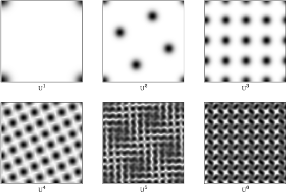
FIG. 1.: Modulo of the coherent state return amplitude for the first six powers of the Arnold cat map propagator. The torus is quantized with periodic boundary conditions, and $N=128$. Linear grey scale between 0 (white), and the maximum (black) of each picture.

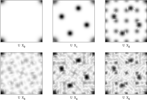
FIG. 2.: Modulo of the coherent state mean value for the $\hat{U}\hat{X}_{n}$ operators. Same parameters and scales as Fig. 1

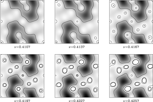
FIG. 3.: Real part of ${\cal H}_{a}(s,z,\bar{z})$, for $s=\exp(-i2\pi\nu)$. Linear grey scale between 0 (white), and $1/\sqrt{N}$ (black). Logarithmic level curves at $1/N,1/N^{2},1/N^{3},...$. Arnold cat map with periodic boundary conditions, and $N=14$. There is an eigenvalue of the propagator near $\nu=0.4167$ (3rd. picture). The exact and semiclassical computation gives the same values.

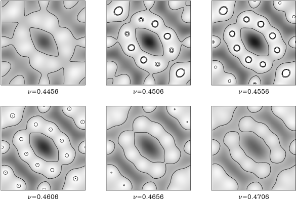
FIG. 4.: The same as Fig. 3, but for the baker map, with anti-periodic boundary conditions, and $N=16$. There is an eigenvalue of the propagator near $\nu=0.4606$ (4th. picture).

FIG. 5.: Exact $Z$ function (bold line), and its semiclassical approximation (dashed line), for the baker map, with anti-periodic boundary conditions, and $N=20$. The zeroes correspond to the eigenvalues

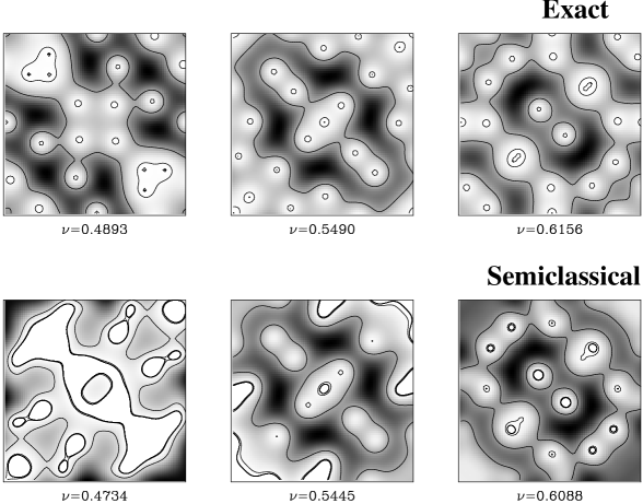
FIG. 6.: Exact and semiclassical eigenstates in correspondence with the zeroes in Fig.5. The gray scale and the contours are as in Fig.3.

REFERENCES

- [1] M. V. Berry, Les Houches Lecture Notes, Summer School on Chaos and quantum Physics, M.-J. Giannoni, A. Voros, and J. Zinn-Austin, eds., Elsevier Science Publishers B. V. (1991); Proc. Roy. Soc. A 243, 219 (1989)
- [2] P. Leboeuf and A. Voros, J. Phys. A 23, 1765 (1990)
- [3] E. J. Heller, Phys. Rev. Lett. 53, 1515 (1984); Wavepacket Dynamics and Quantum Chaology in Chaos and Quantum Physics, M.-J. Giannoni, A. Voros, and J. Zinn-Austin, eds., Elsevier Science Publishers, Amsterdam (1990)
- [4] E. B. Bogomolny Physica D 31, 169 (1988)
- [5] D. A. Wisniacki and E. Vergini, Phys. Rev. E 62, 4513 (2000)
- [6] S. Nonnenmacher, A. Voros J. Stat. Phys. 92, 431 (1998)
- [7] A. D. Mirlin, Lecture course given at the International School Enrico Fermi on New Directions in Quantum Chaos, Varenna, July 1999 (cond-mat/0006421)
- [8] M. C. Gutzwiller, J. Math. Phys. 8, 1979 (1967)
- [9] E. B. Bogomolny and J. P. Keating, Phys. Rev. Lett. 77, 6091 (1994)
- [10] O. Agam and S. Fishman, Phys. Rev. Lett. 73, 806 (1994)
- [11] M. Saraceno and F. Simonotti, Phys. Rev. E 61, 6527 (2000)
- [12] M. V. Berry and J. P. Keating, J. Phys. A 23, 4839 (1990)
- [13] E. B. Bogomolny, Nonlinearity 5, 805 (1992)
- [14] E. B. Bogomolny, O. Bohigas and P. Leboeuf, Phys. Rev. Lett. 68, 2726 (1992)
- [15] M. Marsden, Geometry of Polynomials, American Mathematical Society, Providence, Rhode Island (1966).
- [16] M. V. Berry and J. P. Keating, Proc. Roy. Soc. A 437, 151 (1992)
- [17] A. M. Ozorio de Almeida, Phys. Rep. 295,265 (1998)
- [18] S. Fishman, B. Georgeot and R. E. Prange, J. Phys. A 29, 919 (1996); S. Fishman in Supersymmetry and Trace Formulae: Chaos and Disorder, Lerner et al. Eds., NATO ASI B Vol. 370, Kluwer Academic, New York (1999)
- [19] J. H. Hannay and M. V. Berry, Physica 1D, 267 (1980)
- [20] M. Saraceno and A. Voros, Physica D 79, 206 (1994)