Composite “zigzag” structures in the 1D complex Ginzburg-Landau equation

Abstract

We study the dynamics of the one-dimensional complex Ginzburg Landau equation (CGLE) in the regime where holes and defects organize themselves into composite superstructures which we call zigzags. Extensive numerical simulations of the CGLE reveal a wide range of dynamical zigzag behavior which we summarize in a “phase diagram”. We have performed a numerical linear stability and bifurcation analysis of regular zigzag structures which reveals that traveling zigzags bifurcate from stationary zigzags via a pitchfork bifurcation. This bifurcation changes from supercritical (forward) to subcritical (backward) as a function of the CGLE coefficients, and we show the relevance of this for the “phase diagram”. Our findings indicate that in the zigzag parameter regime of the CGLE, the transition between defect-rich and defect-poor states is governed by bifurcations of the zigzag structures.

PACS: 05.45.Jn, 47.54.+r, 05.45.Pq

and

1 Introduction

Many extended systems display the formation of patterns when driven sufficiently far from equilibrium. In the simplest case, such patterns are regular, but often the patterned state displays disorder in space and time; this phenomenon is referred to as spatiotemporal or extended chaos [1, 2, 3, 4, 5, 6, 7, 8, 9, 10, 11, 12]. The tools to describe chaos in low dimensional systems are often impracticable for the description of extended chaos. In addition, they are not suited for describing the spatial organization that takes place in chaotic states that appear to be built up from local structures, almost particle-like entities with well defined dynamics and interactions [6].

The one-dimensional complex Ginzburg Landau equation

$$\partial_{t}A=A+(1+ic_{1})\partial_{xx}A-(1-ic_{3})|A|^{2}A~{},$$ (1)

describes pattern formation near a supercritical Hopf bifurcation [1] and provides a convenient framework for the study of spatiotemporal chaos and the role of local structures [1, 2, 3, 4, 5, 6, 7, 8, 9, 10, 11, 12]. In the CGLE, a wide range of dynamical states can be reached depending on the coefficients $c_{1}$ and $c_{3}$ and the initial conditions: (i) For small $c_{1}$ and $c_{3}$, plane waves where $A\!\sim\!\exp(i(qx-\omega t))$ are the dynamically relevant states. (ii) For coefficients $c_{1}$ and $c_{3}$ beyond the Benjamin-Feir-Newell curve where $c_{1}c_{3}\!=\!1$, all plane waves are linearly unstable and spatiotemporally chaotic states occur [1, 2, 3, 4, 5, 11]. When one takes sufficiently smooth initial conditions and fixes $c_{1}$ and $c_{3}$ just beyond the Benjamin-Feir-Newell instability, so-called phase chaos occurs. In such states, the value of $|A|$ remains close to unity and the essential dynamics occurs in the complex phase $\phi$ of the order parameter $A$. (iii) For different initial conditions or larger values of $c_{1}$ and $c_{3}$, $A$ can go through zero. At such points the phase gradient diverges and the phase field shows topological defects; chaotic states where this happens are referred to as defect chaos. The transition from phase to defect chaos can either be continuous or hysteretic [4, 5, 7, 10]. Once defects are formed in the hysteretic regime, defect chaos persists down to the so-called $L_{2}$ transition [5].

Near this $L_{2}$ transition, spatiotemporally chaotic states are often built up from holes (propagating local concentrations of the phase-gradient) and defects [8, 9]. In this paper we will study the dynamical states that occur when these holes and defects organize into more complex composite structures called zigzags [8] (see Fig. 1). Zigzags consist of a core where holes alternatingly propagate left and right; in this process holes are periodically emitted from the core. Extensive numerical simulations of the CGLE, presented below, reveal that zigzags display a wide variety of dynamical behaviors. In addition, while most chaotic states of the CGLE are characterized by short-time correlations [4], the relevant time scales of some of the chaotic zigzag states can be of order $10^{3}$ or larger (see Fig. 5 and 6). We develop numerical methods to perform linear stability and bifurcation analysis for these complex structures; these tools are applicable to a wide range of complex local structures such as oscillating sources [13], oscillating domain walls [14] and oscillating pulses [15]. The results of our analysis indicate that, in the zigzag dominated regime, the $L_{2}$ transition is closely related to local bifurcations of the zigzags.

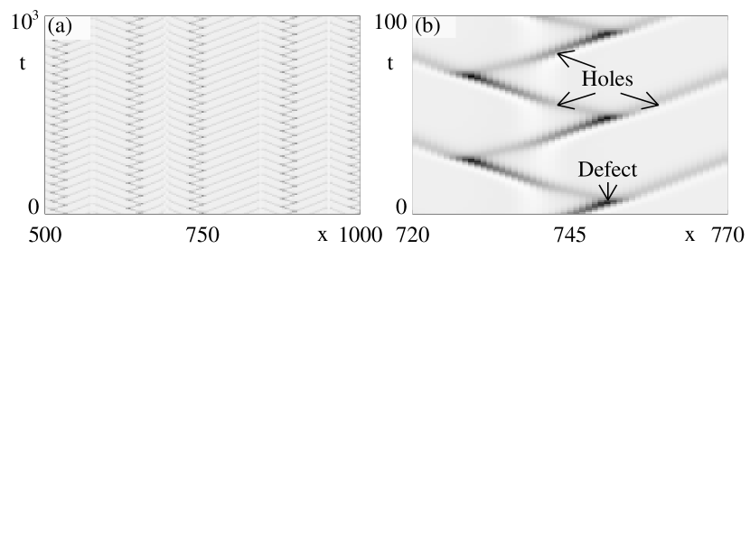
Figure 1: Grey scale (black corresponding to $A\!=\!0$) space–time plots of $|A|$ showing basic zigzag phenomenology. (a) A part of a “frozen” state of many stationary zigzags obtained for $c_{1}\!=\!0.9$ and $c_{3}\!=\!1.15$, in a system of size 2048, starting from random initial conditions. A transient of $t\!=\!10^{4}$ has been removed. (b) Close–up of the core region of a stationary zigzag in (a), identifying the defects and holes.

The paper is organized in two parts. We first study the phenomenology of zigzags, and discuss the role of the holes and defects that constitute their building blocks (section 2). Then we perform a numerically very demanding linear stability and bifurcation analysis of zigzags (section 3)), and show how some of the main features of the zigzag phenomenology can be understood from this analysis.

2 Phenomenology of zigzags

The zigzag structures display a wide variety of dynamical behaviors as a function of the coefficients $c_{1}$ and $c_{3}$ of the CGLE (see Figs. 4–6). In section 2.1 we will discuss the local structures that form the zigzags and discuss various types of regular zigzags. An overview of regular and irregular zigzag dynamics in large systems and for long integration times is presented in section 2.2.

2.1 Ingredients of zigzags: holes and defects

Some of the qualitative properties of zigzags can be understood from the properties of the homoclinic holes and defects that are the building blocks of zigzags and that have been studied in a series of recent papers [8, 9, 10]. The main ingredients of importance here are briefly summarized below. (i) Coherent homoclinic holes are localized packets of phase gradient that have the special property that they can propagate uniformly, i.e., they are of the form $A(x,t)\!=\!\exp{i\omega t}\bar{A}(x-vt)$ [8]. Right (left) moving holes are characterized by a positive (negative) phase gradient peak in their core. (ii) Coherent holes are linearly unstable, and in phase space they form a saddle with a one-dimensional unstable manifold [8]. When they are perturbed so-called incoherent holes are observed, i.e., holes that evolve over time; in phase space we can think of these holes as evolving along the one-dimensional unstable manifold of the coherent holes. Incoherent holes finally either decay or evolve towards defects, and the closer an initial condition is towards the stable manifold of the coherent holes, the longer its lifetime. (iii) The spatial profile that occurs shortly after a defect has occurred consists of a juxtaposition of a negative and positive phase gradient peak. The negative peak can initiate a left moving hole, and the positive peak a right moving hole.

The traveling holes that occur in our zigzag states (see Fig. 2a) are incoherent, and as expected their direction of propagation is governed by the sign of their phase gradient (see Fig. 2a). Let us inspect the zigzag structure in detail, starting from the defect $d_{1}^{-}$ in Fig. 2b. This defect generates two new incoherent holes, $l_{1}^{-}$ and $r_{1}^{-}$. The former stays in the core and rapidly generates another defect $(d_{2}^{+})$, while the latter is send out of the zigzag core. The difference in lifetimes between $l_{1}^{-}$ and $r_{1}^{-}$ is related to the details of the defect profile of $d_{1}^{-}$. In the regime of the CGLE where zigzags occur, the positive peak of a $d^{-}$ defect is closer to the stable manifold of a right moving hole, than the negative peak is to the stable manifold of a left moving hole. As a result, the lifetime of the $r^{-}$ holes is larger than that of $l^{-}$ holes. As far as we understand, this is the essential condition that produces zigzags. The left-right symmetry of the CGLE inverts the sign of phase gradients, implying that the lifetime of an $r$ hole emanating from a $d^{-}$ defect is similar to the lifetime of an $l$ hole emanating from a $d^{+}$ defect. This symmetry can be (weakly) broken, giving rise to drifting zigzags (see below).

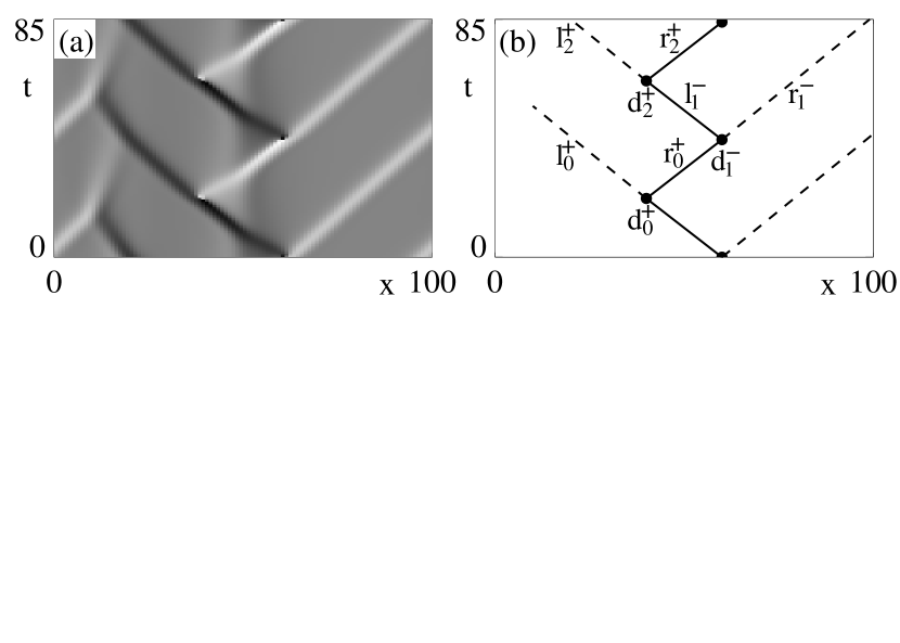
Figure 2: (a) Grey scale plot for the phase gradient for a stationary zigzag. White (black) corresponds to positive (negative) phase gradient; in the grey areas the phase gradient is close to zero. (b) Schematic structure of the same zigzag as in (a). Defects are labeled with a $d^{\pm}$, where the sign reflects the change in winding number $\int dx\partial_{x}\phi$ before and after their occurrence; after the generation of a $d^{+}$ ($d^{-}$) defect the winding number has increased (decreased) by $2\pi$. The holes are labeled $(l,r)$ depending on their direction of propagation, and are created by and evolve to defects. Holes carry the sign of the defect that generated them as an additional label. A left (right) moving hole can only generate $d^{+}$ ($d^{-}$) defects [8, 9].

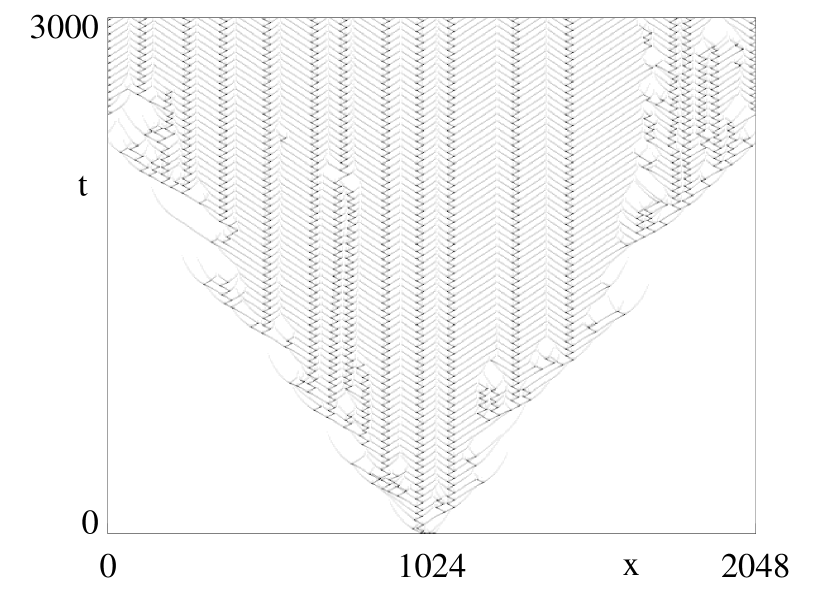
Figure 3: Example of the spreading out of zigzags when the wing holes are active, for $c1\!=\!0.9$ and $c3\!=\!1.15$.

It is important to note that for values of $c_{1}$ and $c_{3}$ away from the zigzag regime, hole-defect dynamics with completely different dynamics may occur. For example, when the time scales of $r^{+}\rightarrow d^{-}$ and $r^{-}\rightarrow d^{-}$ are similar more disordered dynamics as shown in Fig. 1 of [8] sets in, while when $r^{+}\rightarrow d^{-}$ is slower than $r^{-}\rightarrow d^{-}$, the dynamics is dominated by propagating incoherent holes [9].

2.1.1 Wing holes

Holes that are send out of the zigzag core (like hole solutions indicated by $l_{2}^{+}$ and $r_{1}^{-}$ in Fig. 2) are referred to as wing holes. For regular zigzags, the holes a generated periodically, yielding traveling periodic arrays of holes, with hole-hole spacings ranging from 20-100; the size of this spacing is typically sufficient for regarding the holes as isolated. These wing holes can either evolve to defects or decay. In the former case, zigzag dynamics spreads throughout a laminar background (Fig. 3) and holes collide in shock-like structures that separate neighboring zigzags (Fig. 4a); in this case the maximal spacing between zigzags is set by the wing hole lifetime. When the wing holes decay isolated zigzags can occur (Fig. 4b).

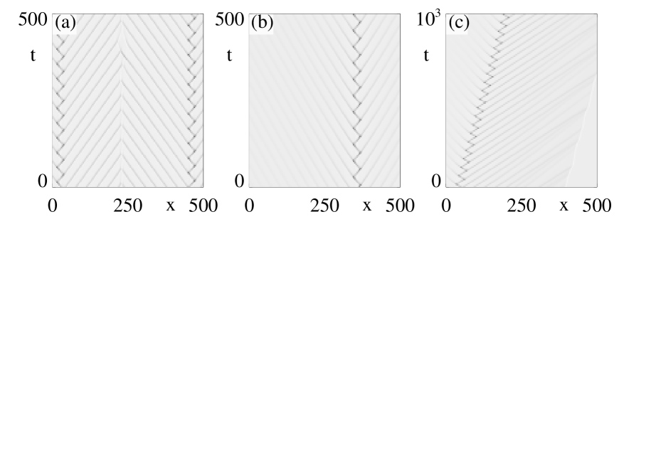
Figure 4: Illustration of the difference between active and decaying wing holes, and stationary and traveling zigzags. All panels show $|A|$ from a longer run in a system of size 2048. (a) Active wing holes for $c_{1}\!=0.9$ and $c_{3}\!=\!1.14$. Here the final states consist of a number of stationary zigzags, separated by a range of distances. Here we show the area in between two widely separated zigzags. For this spacing the wing holes are very close to being critical and for larger separation they would grow out to defects. Some effect of this is seen in the fluctuation near $x\!=\!250$ and $t\!=400$. (b) For $c_{1}\!=\!0.8$ and $c_{3}\!=\!1.13$ the wing holes clearly decay, and zigzags are essentially isolated. (c) The late dynamics in a run for $c_{1}\!=\!0.6$ and $c_{3}\!=\!1.2$, showing an isolated traveling zigzag.

2.1.2 Core holes and drift

A priori one does not know whether the hole-defect composite that makes up the core of the zigzags is linearly stable, although the examples shown in Fig. 1 and 4 clearly indicate that this can be the case. In some cases however, stationary zigzags can become linearly unstable. We will present ample examples of this below, but here we will already point out the main consequence: depending on the CGLE coefficients, stable zigzags can either be stationary (Fig. 4a,b) or drifting (Fig. 4c). In section 3 we will show that the drifting zigzags branch off from the stationary zigzags via a pitchfork bifurcation.

2.2 Large scale zigzag dynamics

We studied zigzag behavior on large domains $(L=2048)$ and for long integration times of the order $10^{4}$ – $10^{5}$, and examples of the different dynamical states that we obtained are presented here.

Here we will present eight qualitatively different examples of zigzag dynamics, starting from random initial conditions. The dynamical states that we will present are characterized by such large spatial and temporal scales that space-time diagrams of the modulus of $A$, such as those shown in Fig. 3, become completely cluttered. We therefore only plot the position of all defects in a space-time plot (for details regarding the algorithm used for the detection of defects, see appendix A). For a single stationary regular zigzag these defects occur alternatingly on two spatial positions (see Fig. 1 and 2). On the time scale shown in Figs. 5 and 6 these individual defects can no longer be distinguished, and zigzag structures show up as two parallel lines.

In Fig. 5 we show four examples of dynamics dominated by traveling zigzags. Panel (a) shows a long transient that occurs when $c_{1}\!=\!0.6$ and $c_{3}\!=\!1.16$ are just below the $L_{2}$ transition. Initially, a few stationary zigzags are created, but these appear linearly unstable and give rise to the formation of a few traveling zigzags. These, however, do not sustain, and after a period of the order $10^{4}$ the dynamics decays back to simple uniform oscillations where $A=\exp{i\omega t}$. When $c_{3}$ is increased to a value of $1.2$, the traveling zigzags become stable, and a state consisting of homogeneously drifting zigzags occurs (Fig. 5b). The positions and overall drift of this state are selected by the initial conditions. Note that for early times a left and right moving zigzag collide (around $x\!=\!1600$) which results in the destruction of the left drifting zigzag. The large spacing between neighboring zigzags indicates that the wing holes decay here, similar to Fig. 1c. When $c_{3}$ is increased even further to a value of $1.25$, more complicated dynamics occurs (Fig. 5c). Left and right drifting zigzags compete, and intermittent collisions between zigzags take place from which new zigzags may be created. In some cases we have observed that similar states after a very long transient may decay into a state similar to Fig. 5b where either left or right drifting zigzags occur. Behavior with similar features occurs for $c_{1}\!=\!1$ and $c_{3}\!=\!1.12$ (Fig. 5d), although the drift of the zigzags here is approximately 10 times slower (notice the difference in time scales between Fig. 5c and d). It is not clear whether or not the states in Fig. 5c–d should be considered qualitatively the same or not, nor what an appropriate order parameter for their description should be. This is of course a general problem that we encounter when we try to classify behavior as rich as that shown in these figures.

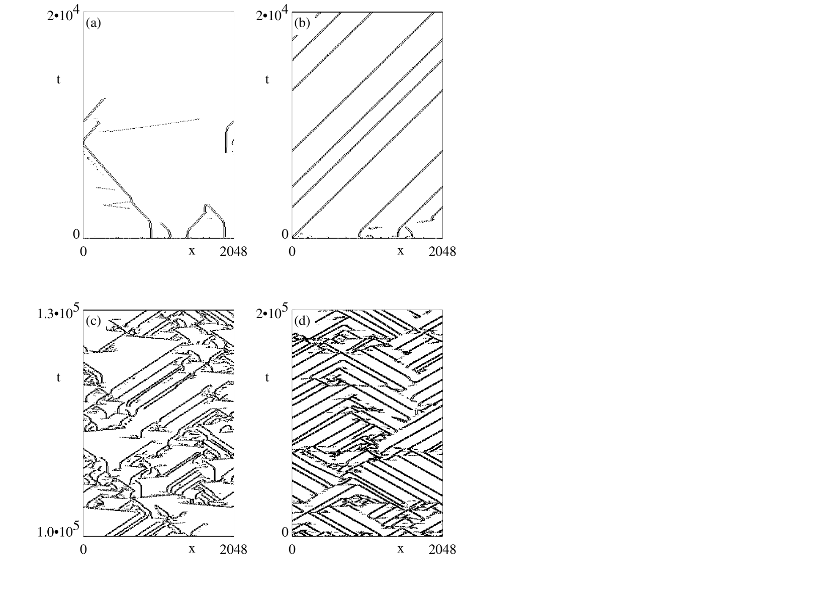
Figure 5: Four examples of zigzag dynamics dominated by drift. (a) $c_{1}\!=\!0.6$, $c_{3}\!=\!1.16$. (b) $c_{1}\!=\!0.6$, $c_{3}\!=\!1.2$. (c) $c_{1}\!=\!0.6$, $c_{3}\!=\!1.25$. (d) $c_{1}\!=\!1.0$, $c_{3}\!=\!1.12$. For more details see text.

Fig. 6 shows four examples of CGLE dynamics dominated by stationary zigzags. For $c_{1}\!=\!0.8$ and $c_{3}\!=\!1.17$ stationary zigzags occur (Fig. 6a). The spacing between adjacent zigzags indicates that the wing holes decay here. In Fig. 6b–d three examples of intermittent zigzag dynamics obtained for $c_{1}\!=\!0.9$ and $c_{3}=1.23$, $1.24$, and $1.25$ are shown. The dynamics in Fig. 6b displays a disordered transient that decays to a stationary “glassy” state of zigzags. Note that the zigzags themselves appear as a substrate on which dynamics on even longer space and time scale occurs; an example is the traveling perturbation seen around $x\!=\!800$ and $t\!=\!4\times 10^{4}$. This suggest a hierarchy of scales: holes and defects form zigzags, zigzags form even larger structures, etc. When $c_{3}$ is increased to 1.24, perturbations of the stationary zigzags do no longer decay, and very disordered dynamics occurs (Fig. 6c). Note however, that stationary zigzags by themselves are not unstable (as evidenced by the large stationary regime in the middle of this figure), but only get perturbed by “contaminations” coming from chaotic patches that spread through the system. This behavior is typical for spatiotemporal intermittency [5]. Finally, when $c_{3}$ is increased even further to a value of $1.25$, the disordered patches become much more dominant, although some pockets filled with stationary zigzags occur (Fig.6d).

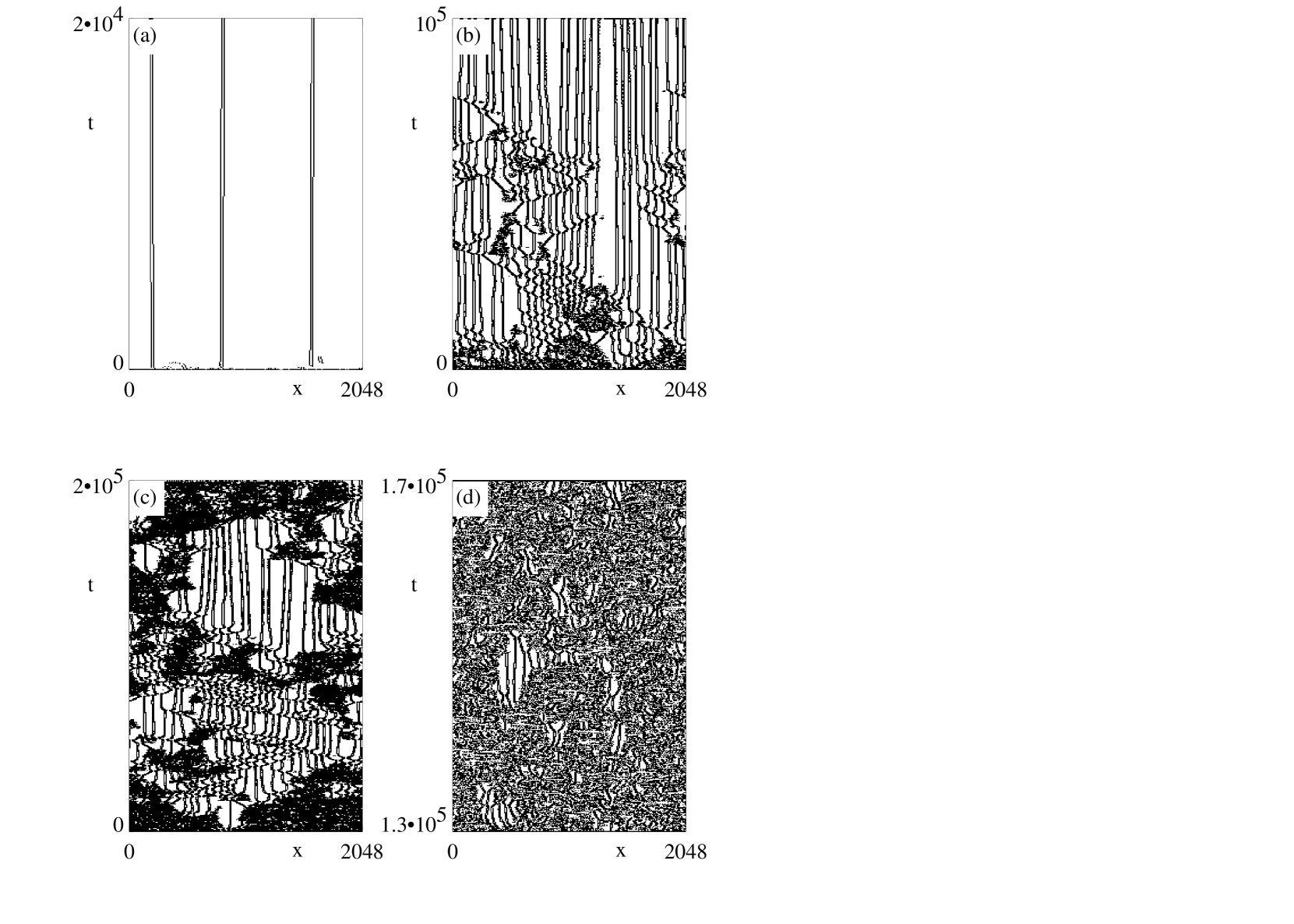
Figure 6: Four examples of dynamics dominated by stationary zigzags. (a) $c_{1}\!=\!0.8$, $c_{3}\!=\!1.17$. (b) $c_{1}\!=\!0.9$, $c_{3}\!=\!1.23$. (c) $c_{1}\!=\!0.9$, $c_{3}\!=\!1.24$. (d) $c_{1}\!=\!0.9$, $c_{3}\!=\!1.25$. For more details see text.

2.2.1 Phase diagram

Based on numerical simulations like the ones presented above, we have attempted to classify the various types of zigzag dynamics into a small number of distinct classes; this results in a “phase diagram” for zigzag behavior (Fig. 7). This diagram constitutes a small part of the full phase diagram of the one-dimensional CGLE only. The simplest state that can be distinguished is where, after a transient, all defects disappear (see Fig. 5a); coefficients for which this happened in our simulations are represented in Fig. 7 by an open circle. States which are dominated by stationary zigzags (like Fig. 6a) are represented by a full circle. Then there are states which are dominated by traveling zigzags (Fig. 5b); these are here represented by a triangle. Even when stationary or traveling zigzags appear to be linearly stable, the overall dynamics can be disordered. In a sense, these states represent examples of what one may call “spatiotemporal intermittency of zigzags”; such intermittent states with stationary zigzags (like those in Fig. 6b–c) are represented by a plus symbol, while intermittent states with traveling zigzags like Fig. 5c–d are represented by a ’$\times$’ symbol. When the coefficients $c_{1}$ and $c_{3}$ are increased sufficiently, pure defect chaos ensues (see Fig. 6d); these states are represented by a star. Finally, one occasionally finds states that do not obviously fall into one of these categories; we have labeled these by boxes.

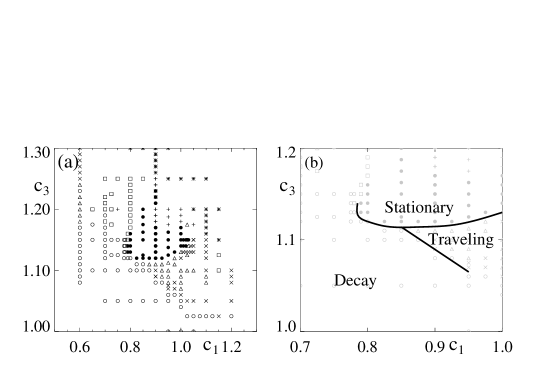
Figure 7: (a) Phase diagram showing the variation of the different zigzags types found in the $c_{1}$ and $c_{3}$ parameter plane. For explanation of symbols: see text. (b) Magnification of (a) showing the main transitions between stationary, traveling and decaying zigzag structures.

It should be noted that for all the points in the phase diagram we performed a single run in a large system ($L=2048$) and for long integration times $T\!=\!10^{5}$, and that each individual run consumes a considerable amount of (super) computing time. Instead of trying to obtain better statistics or a finer spacing of the coefficients for which we performed runs, we have focussed on what we believe is the main feature of the bifurcation diagram (see  Fig. 7b): (i) There exists a finite coefficient regime dominated by stationary zigzags. (ii) At the bottom boundary of this regime, one either finds decaying states or traveling zigzags. The transition between stationary zigzags and decaying or traveling zigzags can be understood from the numerical bifurcation analysis we present in section 3 below.

3 Linear stability and bifurcation analysis

3.1 Stability

We have performed a linear stability analysis of regular zigzag structures to gain some understanding of their large scale dynamics. After the spatial degrees of freedom of the CGLE are discretized, the problem of finding a regular zigzag and its spectrum can be translated into finding a periodic orbit and its spectrum in a set of coupled ODEs. Using standard continuation algorithms, it is then possible to track the spectrum as a function of the coefficients $c_{1}$ or $c_{3}$, thus obtaining stability limits and bifurcation points. This strategy is straight-forward but numerically demanding. For low-dimensional systems of autonomous ODEs, such procedures are standard [16, 17]. Such analysis is already well-described in the literature (see e.g. [18]), but has so far mostly been applied to the study of spatial structures such as uniformly traveling fronts and spots, whose spatio-temporal dynamics is essentially stationary. Here we describe the application of these techniques for structures, such as the zigzags, which are periodic in time.

Symmetries and boundary conditions

The choice of the appropriate frame for the CGLE is essential. To be able to study uniformly drifting zigzag structures we choose a co-moving coordinate frame. During each period of the zigzag the phase of $A$ increases by a global phase shift $\phi$ and the field $A$ is therefore quasiperiodic for a zigzag; however, by going to a “rotating” frame $\sim\mathrm{e}^{\operatorname{i}\phi t}$, $A$ can be made periodic. Hence we study the CGLE in the following form:

$$\partial_{t}A=(1+i\phi)A+v\partial_{x}A+(1+ic_{1})\partial_{xx}A-(1-ic_{3})|A|^{2}A~{},$$ (2)

where $A$ is periodic provided that $\phi$ and $v$ are equal to the global phase shift and the drift velocity of the zigzag. The form of Eq.​ (2) permits us to determine a zigzag numerically by using a shooting algorithm similar to the approach applied when determining limit cycle solutions to autonomous systems of ODEs; for details, see the appendix 2–3. An example of an unstable zigzag determined by this method and its spectrum is shown in Fig. 8.

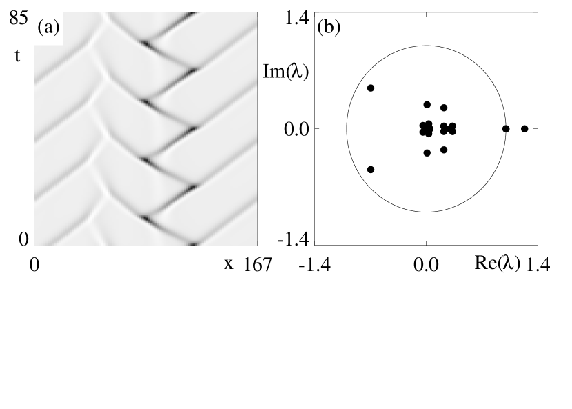
Figure 8: (a) Unstable zigzag obtained for $c_{1}=0.9$ and $c_{3}=1.15$ with period $T=41.64$, global phase shift $\phi=-2.80$, and velocity $v=-0.0218$. The spectrum associated with this zigzag is shown in (b). Note the neutral eigenvalues at $\lambda=1$ and the single unstable eigenvalue.

Due to the periodic boundary conditions wing holes will collide and annihilate in a shock area (see Fig. 8). Their role is unimportant when they are sufficiently far away from the zigzag core, since the group velocity is pointing towards such shocks and no “information” can flow out of them. The position of these shocks is not arbitrary; for the chosen domain sizes, at most a number of discrete spacings between the zigzag core and the shock are available (see Fig. 2b); in general we have chosen our initial and pinning conditions such that the shocks are positioned as far from the zigzag core as possible.

Since coherent holes are linearly unstable, one may wonder whether the corresponding unstable eigenvalues would appear in the spectrum. However, the holes that occur in zigzags are incoherent and have a finite lifetime, because they evolve to defects (as happens in the core) or are annihilated (as happens to the wing holes). It is around these states that one studies the stability now; the linear stability of the hole composite zigzag can only be obtained by studying the full spectrum of the composite structure. Another example where linearly unstable coherent holes give rise to partly regular incoherent hole dynamics can be found in [9].

3.2 Numerical bifurcation analysis of zigzags

In the previous sections, we have already seen that both steady and traveling zigzags exists as stable solutions to the CGLE. Here we discuss how transitions between these two states can be described using the continuation strategy discussed in Section 3 for determining the stability and structural properties of a zigzag pattern.

Throughout, we choose $c_{1}$ and $c_{3}$ as free parameters, and focus on the region in the phase diagram dominated by transitions between regular stationary and traveling zigzags. This corresponds to the region of the phase diagram highlighted in Fig. 7b; In particular, we shall focus on the transitions from stationary to either decaying or traveling zigzags respectively.

We have employed the following strategy: for different fixed values of $c_{1}$, we make a vertical continuation scan through the phase diagram in Fig. 7 by varying $c_{3}$. The results for $c_{1}=0.80,0.85,0.87$, and $0.90$ are shown in  Fig. 9a-d, where the variation of the zigzag velocity $v$ is shown as a function of $c_{3}$. For $c_{1}=0.80$, the stationary zigzag is initially unstable for $c_{3}<1.12$, above which it becomes stabilized via a subcritical pitchfork bifurcation, which gives birth to two unstable branches of left and right traveling zigzags. The perfect symmetry of the pitchfork is slightly perturbed since we work on a spatial domain of finite size. Effectively, this renders the zigzag slightly asymmetric implying that the bifurcation diagram exhibits the typical behavior found near a perturbed pitchfork, where the symmetric “fork” splits into two separate branches containing a fold (saddle-node) point and a simple unbranched state. Since this splitting solely is due to a finite-size effect, we shall refer to the above bifurcation as a “pitchfork” bifurcation. For $c_{1}=0.80$, the stationary zigzag remains stable for $c_{3}<1.16$, where it merges with the branches of the traveling zigzags and looses stability via a second subcritical pitchfork bifurcation (not shown). The location of the lower bifurcation point is in excellent agreement with the transition from stationary to decaying zigzags observed in the phase diagram.

Figure 9: Bifurcation diagrams showing the variation of the zigzag velocity $v$ as a function of $c_{3}$ for $c_{1}=0.80,0.85,0.87$, and $0.90$ corresponding to (a-d) respectively.

Qualitatively, the results for $c_{1}=0.85$ shown in Fig. 9b are similar to the behavior described above, except that the slopes of the bifurcating branches of traveling zigzags near the lower pitchfork point have increased. This suggests that a transition from a sub- to a supercritical pitchfork may occur as $c_{1}$ is increased further. This is confirmed in Fig. 9c, where $c_{1}$ is fixed at $0.87$. Here the branches of traveling zigzags now branch off from the pitchfork point in the direction of decreasing $c_{3}$. As $c_{3}$ decreases further, a fold point is reached at which both of the traveling zigzag solutions are destabilized. Effectively, the transition from sub- to supercriticality generates a parameter region in which traveling zigzags are stable. This region is localized below the region where stable stationary zigzags exist. The change of the bifurcation from sub- to supercritical is in agreement with the emergence of the region of traveling zigzags in the phase diagram. Finally, for $c_{1}=0.90$ the range of $c_{3}$ within which stable traveling zigzags occur increases (see  Fig. 9d) in correspondence with the observation from phase diagram.

4 Discussion

In this paper, we have discussed both the structural and dynamical properties of the family of zigzag solutions of the CGLE. Some of the structural properties of the zigzags can be understood in terms of the properties of their constituent homoclinic holes and defects [8, 9, 10]. To understand our finding that zigzag structures can either be stationary or traveling, we have employed a stability and bifurcation analysis, which shows that the two types of zigzags are related by a pitchfork bifurcation. This analysis also reveals that some of the transitions observed in the zigzag phase diagram are governed by these bifurcations; in particular, some part of the $L_{2}$ transition between defect rich and defect poor dynamics of the CGLE is apparently given by these bifurcations. It is therefore unlikely that a unified description of this $L_{2}$ curve exists.

The existence of parameter regimes where stationary or traveling zigzags act as building blocks for chaotic and intermittent zigzag dynamics occurring on very slow scales (see Fig. 5 and 6) illustrates the amazing richness of the one-dimensional CGLE.

It is a pleasure to acknowledge illuminating discussions with M. Howard. MvH acknowledges financial support from the EU under contract nr. ERBFMBICT 972554. MI acknowledges financial support from the Alexander von Humboldt Stiftung, Germany.

Appendix A appendix

A.1 Numerical defect detection

Figure 10: Illustration of our defect detection algorithm. The open circles represent four points of our discretized lattice, and the dashed line indicates the loop integral. (a) Regular case, no branch lines. (b) When no defects are present, a branch line intersects the loop twice. (c) A defect within the loop gives rise to a single intersection with the branch line. For further details see text.

Detecting defects in a phase field defined on a discrete space-time grid is not completely trivial since the phase variable $\phi$ is defined modulo 2$\pi$ only. Even for a smooth phase field, $\phi$ jumps by 2$\pi$ along branch lines, and it is difficult to distinguish between such branch lines and large “physical” gradients of $\phi$. A simple and robust method to detect defects is illustrated in Fig. 10. If we assume that the discretization is fine enough then the phase differences between neighboring points should also be small. Hence we require that $|\phi_{2}-\phi_{1}|$ is less than $\pi$. If we find a larger difference, we assume that this is because a branch line crosses between these two points (as in Fig. 10b), and we simply add or subtract a correction of $2\pi$ to this difference. Obviously, a branch line will cut twice through the loop shown in Fig. 10b; the two corrections cancel, and our loop integral will be zero. However, when a defect is present within this loop, the branch line emanating from this defect will intersect the loop only once (Fig. 10c), and the addition of the corrections along this loop yields that the loop integral is plus or minus $2\pi$. A stable and fast algorithm to detect defects is thus to mark the bonds in our space-time lattice where absolute values of the phase difference between adjacent points are larger then $\pi$ by $\pm 1$, and then perform the loop integrals over these bond variables.

A.2 Numerical integration

To be able to explore the CGLE for large domains and integration times, we have chosen a simple next-neighbor, finite difference scheme, where the resulting set of ODEs are integrated using an explicit 4th. order Runge-Kutta scheme with an adaptive time step [19]. We have taken a spatial resolution of $\Delta x=1$ and the time step remains smaller than 0.05 in general. Clearly, such a code sacrifices accuracy for speed; we have no indications, however, that the qualitative zigzag behavior is very sensitive to this. The stability analysis described in section 3 uses the same integrator to facilitate direct comparison between CGLE behavior and the linear stability of the zigzags, and a more refined spatial grid would increase the number of degrees of freedom used in the stability analysis beyond what we can handle numerically.

A.3 Linear stability calculations

By discretization of space the linear stability problem for zigzags has been converted into a shooting problem for the corresponding ODEs. To obtain a well-defined problem, we add three pinning equations for the three unknowns corresponding to the period $T$, the global phase shift $\phi$ and the velocity $v$. If the one-dimensional spatial domain is discretized into $n$ equidistant grid points, after integrating for a period $T$ we obtain $2n+3$ real equations in $2n+3$ real unknowns which may be solved by a standard Newton iteration procedure. Therefore the corresponding Jacobian must be be evaluated. An accurate numerical determination of the Jacobian matrix can be found by solving the variational equations associated with the discretized CGLE for the respective variables and parameters [22]. For the numerical integration of these variational equations, we used the explicit solver from the LSODE package [23], and then linked the solver directly to a standard continuation package [24], which allowed the parametric dependence to be determined. Note that for a spatial domain discretized into $n$ grid points, the integration of the variational equations requires solving a system of $2n(2n+1)$ coupled ODEs, which for the problem discussed here typically is of the order $40000$!

Figure 11: Comparison between the real and imaginary parts of the zigzag eigenmodes associated with the phase invariance (a-b), translational invariance of time and space (c-d) and (e-f), for the CGLE for $c_{1}=0.9$ and $c_{3}=1.15$. Numerical obtained modes are indicated by symbols, while the predicted modes are given by closed curves.

The local stability properties of the periodic solutions thus obtained are described by Floquet theory [25]. The time dependent variation of local perturbations of the limit cycle after the evolution of each period along the orbit is governed by the monodromy matrix $M$, which can be obtained as a by-product from the solution of the variational equations after each successful convergence of a continuation step [22]. The eigenvalues of the monodromy matrix are the Floquet multipliers and describe the growth or decay of perturbations of our limit cycle; loosely they are referred to as the “spectrum” of the corresponding zigzags. For a given set of parameters, the condition $\lvert\lambda\rvert=1$, designate bifurcation points where zigzags change stability.

For limit cycle solutions of systems of autonomous ODEs, one multiplier will always satisfy $\lambda=1$ due to the time translational invariance of the periodic orbit. Additional invariances appear for the problem considered here. Due to phase invariance $\operatorname{i}A$ is a neutral eigenmode associated with a multiplier $\lambda=1$. Furthermore, due to the periodic boundary conditions, the spatial translational mode given by the gradient $\partial_{x}A$ of the complex field also corresponds to a neutral mode. We should therefore have three neutral modes, and this provides a convenient check for the numerical accuracy of the calculated monodromy matrix.

Here we discuss the case $c_{1}=0.9$ and $c_{3}=1.15$, corresponding to the zigzag pattern shown in Fig. 8. The respective neutral Floquet multipliers associated with the described modes, differ from unity by $1.706\cdot 10^{-4}$, $1.905\cdot 10^{-6}$, $9.559\cdot 10^{-4}$ for time, space, and phase invariant modes respectively. Since the eigenmodes associated with these particular multipliers are known, we may compare these with the corresponding eigenmodes obtained numerically from the monodromy matrix. In Fig. 11a-f we compare the numerically calculated neutral eigenmodes with the predictions; the agreement is quite close. The main deviations between the calculation and prediction are observed in the spatial translation mode. This is likely due to the rather coarse discretization used in our numerics ($\Delta x=1$).

References

- [1] M. C. Cross, P. C. Hohenberg, Pattern formation outside of equilibrium, Rev. Mod. Phys. 65 (3) (1993) 851–1112.
- [2] H. Sakaguchi, Phase turbulence and mutual entrainment in a coupled oscillator system, Prog. Theor. Phys. 83 (1990) 169–174.
- [3] H. Sakaguchi, Breakdown of the phase dynamics, Prog. Theor. Phys. 84 (1990) 792–800.
- [4] B. I. Shraiman, A. Pumir, W. van Saarloos, P. C. Hohenberg, H. Chaté, M. Holen, Spatiotemporal chaos in the one-dimensional complex Ginzburg-Landau equation, Physica D 57 (1992) 241–248.
- [5] H. Chaté, Spatiotemporal intermittency regimes of the one-dimensional complex Ginzburg-Landau equation, Nonlinearity 7 (1994) 185–204.
- [6] H. Chaté, On the analysis of spatiotemporally chaotic data, Physica D 86 (1995) 238–247.
- [7] D. A. Egolf, H. S. Greenside, Characterization of the transition from defect to phase turbulence, Phys. Rev. Lett. 74 (1995) 1751–1754.
- [8] M. van Hecke, Building blocks of spatiotemporal intermittency, Phys. Rev. Lett. 80 (1998) 1896–1899.
- [9] M. van Hecke, M. Howard, Ordered and self-disordered dynamics of holes and defects in the one-dimensional complex ginzburg-landau equation, arXiv.org e-Print archive, nlin.CD/0002031.
- [10] L. Brusch, M. G. Zimmermann, M. van Hecke, M. Bär, A. Torcini, Modulated amplitude waves and the transition from phase to defect chaos, Phys. Rev. Lett. 85 (2000) 86–89.
- [11] L. Kramer, I. Aranson, The world of complex Ginzburg-Landau equation, submitted to Rev. Mod. Phys.
- [12] W. van Saarloos, P. C. Hohenberg, Fronts, pulses, sources and sinks in generalized complex Ginzburg-Landau equations, Physica D 56 (1992) 303, see also errata in [26].
- [13] M. van Hecke, C. Storm, W. van Saarloos, Sources, sinks and wavenumber selection in coupled CGL equations and experimental implications for counter-propagating wave systems, Physica D 134 (1999) 1.
- [14] M. van Hecke, B. A. Malomed, A domain wall between single-mode and bimodal states and its transition to dynamical behavior in inhomogeneous systems, Physica D 101 (1997) 131–156.
- [15] R. J. Deissler, H. R. Brand, Periodic, quasi-periodic, and chaotic localized solutions of the quintic complex Ginzburg-Landau equation, Phys. Rev. Lett. 72 (1994) 478–481.
- [16] E. J. Doedel, A. R. Champneys, T. F. Fairgrieve, Y. A. Kuznetsov, B. Sandstede, X. Wang, AUTO 97: Continuation and Bifurcation Software for Ordinary Differential Equations (with HomCont) (1997).
- [17] Y. A. Kuznetsov, Elements of Applied Bifurcation Theory, Springer-Verlag, New York, 1995.
- [18] M. Or-Guil, I. G. Kevrekedis, M. Bär, Stable bound states of pulses in an excitable medium, Physica D 135 (2000) 154–174.
- [19] W. H. Press, S. A. Teukolsky, W. T. Vetterling, B. P. Flannery, Numerical Recipes in C, 2nd Edition, Cambridge University Press, New York, 1992.
- [20] K. Lust, D. Roose, A. Spence, A. R. Champneys, An adaptive Newton-Picard algorithm with subspace iteration for computing periodic solutions, SIAM Journal on Scientific Computing 19 (4) (1998) 1188–1209.
- [21] K. Lust, D. Roose, Computation and bifurcation analysis of periodic solutions of large-scale systems, in: E. Doedel, L. S. Tuckerman (Eds.), Numerical Methods for Bifurcation Problems and Large-Scale Dynamical Systems, Vol. 119 of The IMA Volumes in Mathematics and its Applications, Springer-Verlag, 2000, (see also IMA Preprint 1536).
- [22] M. Kub ček, M. Marek, Computational Methods in Bifurcation Theory and Dissipative Structures, Springer-Verlag, New York, 1983.
- [23] A. C. Hindmarsh, OdePack, a systematized collection of ODE solvers, in: R S Stepleman et al. (Ed.), Scientific Computing, North-Holland, Amsterdam, 1983, pp. 55–64.
- [24] M. Marek, I. Schreiber, Chaotic Behavior of Deterministic Dissipative Systems, Cambridge University Press, Cambridge, 1995.
- [25] G. Iooss, D. D. Joseph, Elementary Stability and Bifurcation Theory, 2nd Edition, Springer-Verlag, New York, 1980,1990.
- [26] W. van Saarloos, P. C. Hohenberg, Fronts, pulses, sources and sinks in generalized complex Ginzburg-Landau equations, Physica D 69 (1993) 209, errata.