Anticipated synchronization in coupled chaotic maps with delays

Abstract

We study the synchronization of two chaotic maps with unidirectional (master-slave) coupling. Both maps have an intrinsic delay $n_{1}$, and coupling acts with a delay $n_{2}$. Depending on the sign of the difference $n_{1}-n_{2}$, the slave map can synchronize to a future or a past state of the master system. The stability properties of the synchronized state are studied analytically, and we find that they are independent of the coupling delay $n_{2}$. These results are compared with numerical simulations of a delayed map that arises from discretization of the Ikeda delay-differential equation. We show that the critical value of the coupling strength above which synchronization is stable becomes independent of the delay $n_{1}$ for large delays.

,

1 Introduction

Time-delay systems have attracted a lot of attention in recent years, in part due to the fact that multistability, i.e. the coexistence of multiple attractors, is a common occurrence when the delays are large –typically, much larger than the response time of the system [1]. Interest in multistability arises because multistable systems play a key role in pattern recognition processes [2] and memory storage devices. By choosing appropriate initial conditions, prescribed periodic solutions can be stored as oscillatory patterns of a time-delay system [3, 4, 5]. Synchronization of chaotic time-delay systems has also received attention, since it has potential applications to secure communications [6, 7]. Perez and Cerdeira [8] have shown that, in low-dimensional chaotic systems, a hidden message can be unmasked by the dynamical reconstruction of the chaotic signal using nonlinear dynamical methods. Encrypting a message in the chaotic output of a time-delay system has the advantage that the dynamics is in this case high-dimensional (the dimension increases linearly with the delay [9]) but, in spite of this fact, synchronization can be achieved by transmitting a single scalar signal. Unfortunately, this method is not as secure as initially expected, since it has been shown that by using a special embedding space, the delay time can be identified, and the message can be successfully unmasked [10]. Coupled oscillators with time delays in the coupling, which represent interactions being transmitted at finite speed, have been extensively studied as well [11, 12, 13].

Recently, a new effect of delayed coupling was reported by Voss [14, 15], who showed the existence of an anticipating synchronization regime. In this regime, the slave system becomes synchronized to the chaotic future state of the master system. Anticipation occurs when the coupling is delayed, and results from the interplay of memory effects and relaxation mechanisms. Numerically, this regime was found in coupled semiconductor lasers with optical feedback [16].

In this paper we investigate the existence and stability of anticipated synchronization in coupled time-delay maps, which have the advantage of allowing for analytical calculations. In the next section, we introduce a system of two time-delay coupled maps in a master-slave configuration, and present analytical results on the stability of anticipated and retarded synchronization for generic maps. In Section 3, we apply the results to a delay map that arises from the discretization of the Ikeda delay-differential equation. Section 4 presents a summary and the conclusions.

2 Master-slave coupled delay maps

We consider a one-dimensional map of the form

$$x_{n+1}=bx_{n}+f(x_{n-n_{1}}).$$ (1)

For $|b|<1$, the first term in the right-hand side represents a relaxation mechanism. Under its sole action $x_{n}$ would asymptotically vanish. This relaxation, however, competes with the effect of the nonlinear function $f(x)$, which has the form of a time-delayed feedback with delay $n_{1}$.

The (master) map (1) is used to partially drive the evolution of a new (slave) system $y_{n}$. The dynamics of this system is, in principle, the same as for $x_{n}$, except that a part of the nonlinear component is replaced by the evolution of $x_{n}$, namely

$$y_{n+1}=by_{n}+(1-\eta)f(y_{n-n_{1}})+\eta f(x_{n-n_{2}}).$$ (2)

The parameter $\eta\in[0,1]$ measures the strength of the driving action. Note that $x_{n}$ enters the dynamics of $y_{n}$ with a delay $n_{2}$. This form of unidirectional time-delay coupling is not only an extension to maps of the configuration proposed by Voss for continuous-time systems [10], but also generalizes the master-slave interaction by introducing a parameter ($\eta$) that controls its strength. Voss’s configuration corresponds to the extreme value $\eta=1$.

The structure of Eqs. (1) and (2) suggests that, if driving is effective enough, $y_{n}$ may become synchronized to the driving signal, in the form

$$y_{n}=x_{n-n_{2}+n_{1}}.$$ (3)

If this synchronization is realized, the dynamics of $y_{n}$ coincides with that of $x_{n}$ up to a time shift $n_{1}-n_{2}$. If $n_{1}>n_{2}$ the slave system anticipates the evolution of the master system, and we have anticipated synchronization. On the other hand, if $n_{1}<n_{2}$ the synchronization is retarded.

Linear stability of the synchronized state (3) can be analyzed in the usual way. Taking $y_{n}=x_{n-n_{2}+n_{1}}+\delta y_{n}$, the evolution of the deviation $\delta y_{n}$ in the limit of infinitesimal deviations is readily derived from (2):

$$\delta y_{n+1}=b\delta y_{n}+(1-\eta)f^{\prime}(x_{n-n_{2}})\delta y_{n-n_{1}},$$ (4)

with $f^{\prime}\equiv df/dx$. Note that, if $|b|<1$ and for $\eta=1$, the deviation decreases exponentially with time and synchronization is therefore stable. In view of well-known properties of synchronization in coupled maps without delays, it is possible to advance that, if the dynamics of $x_{n}$ is chaotic, the synchronized state (3) will be stable above a certain threshold $\eta_{c}<1$. On the other hand, if $x_{n}$ is nonchaotic, synchronization should be stable for any $\eta>0$.

For $n_{1}\neq 0$, Eq. (4) can be formally integrated by introducing a linear $(n_{1}+1)$-dimensional map for a variable ${\bf z}_{n}=(z^{0}_{n},z^{1}_{n},\dots,z^{n_{1}}_{n})$, with $z^{k}_{n}=\delta y_{n-k}$. This equivalent map is given by

$${\bf z}_{n+1}=M_{n}{\bf z}_{n},$$ (5)

where the elements of the matrix $M_{n}$ read

$$M_{n}^{i,j}=\left\{\begin{array}[]{ll}b&\mbox{if $i=j=0$,}\\ (1-\eta)f^{\prime}(x_{n-n_{2}})&\mbox{if $i=0,j=n_{1}$,}\\ 1&\mbox{if $i=j+1$ $(j=0,\dots,n_{1}-1)$,}\\ 0&\mbox{otherwise.}\end{array}\right.$$ (6)

The deviations given by Eq. (4) can then be obtained from the solution of the equivalent map,

$${\bf z}_{n}=U_{n}{\bf z}_{0}=M_{n-1}M_{n-2}\cdots M_{1}M_{0}{\bf z}_{0}.$$ (7)

Thus, synchronization is linearly stable if all the eigenvalues of the evolution matrix $U_{n}$ vanish for $n\to\infty$. For $\eta=1$ the eigenvalues are $(b^{n},0,\dots,0)$. For $\eta<1$, on the other hand, $U_{n}$ and its eigenvalues must be calculated numerically, since they involve the successive states of the variable $x_{n}$, cf. Eq. (6). It is interesting to point out that stability is determined by the asymptotic properties of $U_{n}$ in the limit $n\to\infty$, where the driving system $x_{n}$ has exhaustively explored the accessible region of phase space. In this limit, thus, the delay $n_{2}$ of Eq. (2) plays no role in the determination the eigenvalues of $U_{n}$. In consequence, $n_{2}$ is irrelevant to the stability of the synchronized state.

3 Application to the Ikeda delay map

In this section we present numerical results corresponding to maps (1) and (2), with $f(x)=a\sin x$. With this choice of $f(x)$, we refer to Eq. (1) as the Ikeda delay map, since it arises from the discretization of the Ikeda delay-differential equation [1, 17],

$$\dot{x}=-x+\alpha\sin x(t-\tau).$$ (8)

This equation was introduced to describe the dynamics of an optical bistable resonator, where the finiteness of the speed of light is relevant, and therefore require a description that incorporates explicitly the round-trip time of light in an optical cavity. Physically, $x$ is the phase lag of the electric field across the resonator, $\alpha$ is the laser intensity injected into the system, and $\tau$ is the round trip time of the light in the resonator.

Writing $\dot{x}\equiv[x(t+\Delta t)-x(t)]/\Delta t$, $t\equiv n\Delta t$, and $\tau\equiv n_{1}\Delta t$, the Ikeda delay map is obtained from Eq. (8) with $b\equiv 1-\Delta t$, $a\equiv\alpha\Delta t$, and $x_{n}\equiv x(t)$. The Ikeda delay map is not to be confused with the discrete Ikeda map [1, 18], which is obtained from (8) by discretizing time in units of $\tau$ in the singular limit where the delay-to-response time ratio diverges.

In the following, we focus the attention on the case $b=0.9$. Our numerical calculations are restricted to random initial condition in $(-\pi,\pi)$ both for the master and the slave system. In Fig. 1 we illustrate anticipated synchronization, for $n_{1}=15$ and $n_{2}=0$. The slave system (dashed line) anticipates in $15$ steps the state of the master system (solid line). After a transient, the difference $x_{n+n_{1}-n_{2}}-y_{n}$ (dotted line) decays to zero. We have verified that this behavior is independent of the value of $n_{2}$.

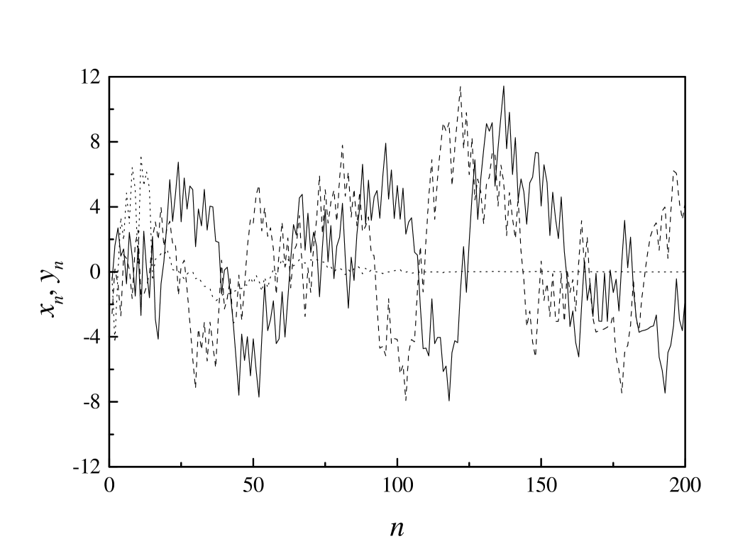
Figure 1: Time series of the maps (1) ($x_{n}$, solid line) and (2) ($y_{n}$, dashed line) with $f(x)=a\sin x$, for $a=3$, $b=0.9$, $\eta=0.833$, $n_{1}=15$, and $n_{2}=0$. The dotted line stands for the difference $x_{n+n_{1}-n_{2}}-y_{n}$.

The critical value $\eta_{c}$ of the coupling strength, above which the synchronized state is stable, has been calculated from the analytical results of the previous section by means of a numerical evaluation of the matrix $U_{n}$ in Eq. (7). Since the delay $n_{2}$ is irrelevant to this calculation, we can take $n_{2}=0$ in Eq. (6). From a given initial condition for the master system, the matrix $U_{n}$ is evaluated for successive values of $n$. In order to avoid the calculation of its eigenvalues, which is specially troublesome for large $n_{1}$, $U_{n}$ is multiplied at each step by a randomly generated vector, ${\bf u}_{n}$, of unitary modulus. If, for a given value of $\eta$, the modulus of the product remains above a certain upper threshold $H$ for sufficiently large $n$, $|U_{n}{\bf u}_{n}|>H$ for $n>n_{\max}$, synchronization is considered unstable and $\eta_{c}>\eta$. If, on the other hand, $|U_{n}{\bf u}_{n}|<h$ for $n>n_{\max}$, where $h$ is a suitable lower threshold, synchronization is considered stable and $\eta_{c}<\eta$. With this criterion, $\eta_{c}$ can be found by decimation within the interval $(0,1)$ up to a certain previously fixed precision. In our calculations, we have taken $H=10^{10}$, $h=10^{-10}$, and $n_{\max}\sim 10^{4}$.

Figure 2 shows $\eta_{c}$ as a function of the delay $n_{1}$ and for several values of the parameter $a$. Note that for small $n_{1}$ –specifically, for $n_{1}=1$– the critical value $\eta_{c}$ can vanish, which indicates that the master evolution is nonchaotic. Notice, furthermore, that for some values of $a$ and $n_{1}=1$ we have plotted more than one value of $\eta_{c}$. This is due to the fact that, in such cases, the master system is multistable –with, typically, two chaotic attractors. The value of $\eta_{c}$ depends thus on the initial conditions for both $x_{n}$ and $y_{n}$. Whereas the behavior is quite irregular for small $n_{1}$, for larger delays the critical coupling becomes practically independent of $n_{1}$. Though it has not been possible to prove this analytically, we conjecture that $\eta_{c}$ approaches a finite limit below unity as $n_{1}\to\infty$. The dependence on $a$ in the investigated interval is also moderately weak. As expected, since the dynamics of the Ikeda delay map becomes more irregular as $a$ grows –i.e. the Lyapunov exponent is higher– $\eta_{c}$ increases accordingly.

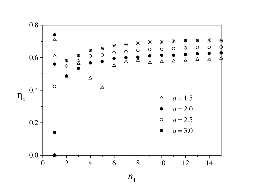
Figure 2: Critical value of the coupling strength above which the synchronized state is stable, calculated by means of a numerical evaluation of the matrix $U_{n}$ in Eq. (7), as explained in the text.

The degree of anticipated of retarded synchronization can be quantified by calculating the similarity function $S_{j}$, defined as [19]:

$$S_{j}^{2}={{\langle[x_{n+j}-y_{n}]^{2}\rangle}\over{[\langle x_{n}^{2}\rangle\langle y_{n}^{2}\rangle]^{1/2}}}.$$ (9)

If $x_{n}$ and $y_{n}$ are independent time series with similar mean value and dispersion, the average of their square difference is of order $2\langle x_{n}^{2}\rangle\approx 2\langle y_{n}^{2}\rangle$, and thus $S_{j}\approx\sqrt{2}\approx 1.4$. If, on the other hand, there is perfect anticipated or retarded synchronization, the difference $x_{n+n_{1}-n_{2}}-y_{n}$ vanishes, and $S_{n_{1}-n_{2}}=0$. In Fig. 3, the similarity function is shown for the same parameters as in Fig. 1.

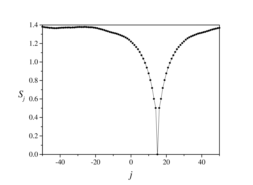
Figure 3: Similarity function, Eq. (9), for the same parameters as in Fig. 1 ($n_{1}-n_{2}=15$).

Figure 4 shows $\min(S)$ –i.e. the minimum value of $S_{n_{1}-n_{2}}$ recorded during sufficiently long realizations of the evolution for a given set of parameters– in the $(n_{1},\eta)$-plane, with all the other parameters as in Fig. 1. The region where anticipated synchronization occurs, $\min(S)\approx 0$, is clearly visible for large values of $\eta$. The position of its boundary is in good qualitative agreement with the values of $\eta_{c}$ shown in Fig. 2 for $a=3$.

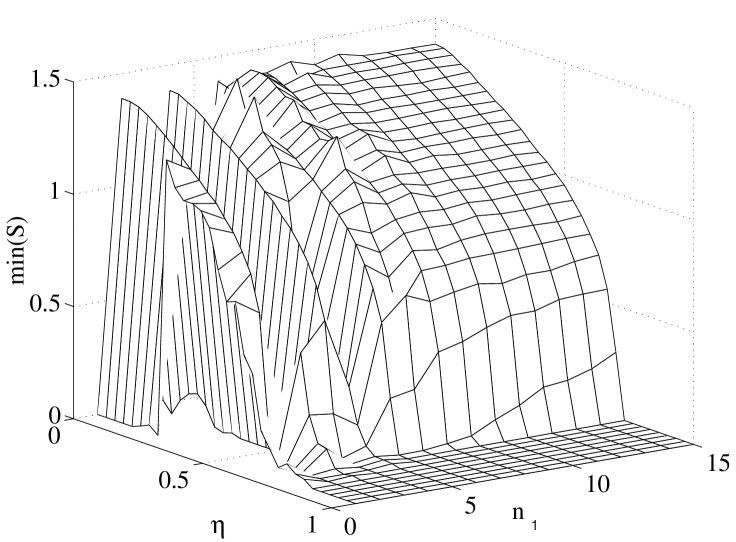
Figure 4: Minimum of the similarity function in the parameter space ($\eta,n_{1}$), with all the other parameters as in Fig. 1. The minimum was calculated by averaging over $50$ trajectories with different initial conditions.

4 Conclusion

We have extended the study of anticipated synchronization, advanced by Voss for unidirectionally coupled differential equations with time delays [14, 15], to delayed coupled chaotic maps. While the nature of anticipated synchronization of maps and differential equations is the same, delay discrete-time dynamics admits an analytical treatment which cannot be carried out for continuous-time systems. In fact, ordinary differential equations with finite time delays constitute an infinite-dimensional problem. On the other hand, since times delays in maps must be discrete, the dimensionality of the problem remains finite.

Taking advantage of this situation, we have analytically studied the stability of anticipated and retarded synchronization in a generic master-slave configuration. In the absence of coupling, master and slave dynamics are identical and involve an intrinsic delay $n_{1}$. Coupling consists in the replacement of a part of the slave dynamics by that of the master system, with a delay $n_{2}$. We have shown that the stability of synchronization is independent of $n_{2}$. The structure of the linearized problem, Eqs. (4-7), suggest meanwhile a strong –though not transparent– dependence on the Lyapunov exponent of the master system, as expected. In practice, the linearized problem has to be treated numerically, but it only involves the realization of the master system and the successive application of the linear-evolution operator, being thus a purely algebraic process.

These results have been applied to the Ikeda delay map, which derives from the application of the Euler integration scheme to the Ikeda delay-differential equation. We have calculated the critical coupling intensity above which synchronization is stable, as a function of the delay $n_{1}$ and of a parameter $a$ that controls the chaotic dynamics of the map. It is found that, whereas for small values of $n_{1}$ the critical coupling can vary considerably –due to the irregular appearance and disappearance of chaotic and nonchaotic attractors– the dependence for large $n_{1}$ is much smoother. In fact, as $n_{1}$ grows, the critical coupling seems to approach a constant value. The dependence with the dynamical parameter $a$ is also moderate in the considered range.

In this work we have focused the attention on exact anticipated synchronization. However, it has been previously shown that approximate anticipated synchronization is possible in coupled differential equations, even in the absence of intrinsic delays [15]. The study of approximate anticipated synchronization in coupled maps constitutes therefore a line for future work. In particular, it would be interesting to investigate in detail the connection between the degree of synchronization, and the irregularity of the dynamics –as measured by the Lyapunov exponents. For delay differential equations, the number of positive Lyapunov exponents and the fractal dimension increase linearly with the delay, while the metric entropy remains roughly constant [9, 20, 21]. We therefore conjecture that the metric entropy might be a good indicator of the possibility of synchronizing with anticipation, and thus predicting, chaotic dynamics.

References

- [1] K. Ikeda, K. Matsumoto, Physica D 29 (1987) 223-235.
- [2] S. Kim, S. H. Park, C. S. Ryu, Phys. Rev. Lett. 79 (1997) 2911-2914.
- [3] B. Mensour, A. Longtin, Phys. Lett. A 205 (1995) 18-24
- [4] J. Foss, A. Longtin, B. Mensour, J. Milton, Phys. Rev. Lett. 76 (1996) 708-711.
- [5] B. Mensour, A. Longtin, Phys. Rev. E 58 (1998) 410-422.
- [6] M. J. Bunner, W. Just, Phys. Rev. E 58 (1998) R4072-R4075
- [7] R. He, P. G. Vaidya, Phys. Rev. E 59 (1999) 4048-4051
- [8] G. Perez, H. A. Cerdeira, Phys. Rev. Lett. 74 (1995) 1970-1973.
- [9] J. D. Farmer, Physica D 4 (1982) 366-393.
- [10] C. Zhou, C.-H. Lai, Phys. Rev. E 60 (1999) 320-323
- [11] M. Y. Choi, H. J. Kim, D. Kim, H. Hong, Phys. Rev. E 61 (2000) 371-381.
- [12] D. Zanette, Phys. Rev. E 62 (2000) 3167-3172.
- [13] D. V. Raman Reddy, A. Sen, G. L. Johnston, Phys. Rev. Lett. 85 (2000) 3381-3384.
- [14] H. U. Voss, Phys. Rev. E 61 (2000) 5115-5119.
- [15] H. U. Voss, Phys. Lett. A 279 (2001) 207-214.
- [16] C. Masoller, Phys. Rev. Lett. 86 (2001) 2782-2785.
- [17] K. Ikeda, H. Daido, and O. Akimoto, Phys. Rev. Lett. 45 (1980) 709-712.
- [18] P. Mandel, Theoretical Problems in Cavity Nonlinear Optics, Cambridge University Press, New York, 1997, and references therein.
- [19] M. G. Rosenblum, A. S. Pikovsky, J. Kurths, Phys. Rev. Lett. 78 (1997) 4193-4196.
- [20] M. Le Berre, E. Ressayre, A. Tallet, H. M. Gibbs, Phys. Rev. Lett. 56 (1986) 274-277.
- [21] C. Masoller, Chaos 7 (1997) 455-462.