Transition from oscillatory to excitable regime in a system forced at three times its natural frequency

Abstract

The effect of a temporal modulation at three times the critical frequency on a Hopf bifurcation is studied in the framework of amplitude equations. We consider a complex Ginzburg-Landau equation with an extra quadratic term, resulting from the strong coupling between the external field and the unstable modes. We show that, by increasing the intensity of the forcing, one passes from an oscillatory regime to an excitable one with three equivalent frequency locked states. In the oscillatory regime, topological defects are one-armed phase spirals, while in the excitable regime they correspond to three-armed excitable amplitude spirals. Analytical results show that the transition between these two regimes occurs at a critical value of the forcing intensity. The transition between phase and amplitude spirals is confirmed by numerical analysis and it might be observed in periodically forced reaction-diffusion systems.

I Introduction

In many cases, the nucleation of spatio-temporal patterns is associated with continuous symmetry breaking, and these patterns are thus very sensitive even to small perturbations or external fields. Perturbations may be induced by imperfections of the system itself (e.g. impurities), of the geometrical set-up (e.g. the boundary conditions), of the control parameters, etc. In addition, external fields may induce spatial or temporal modulations of the control or bifurcation parameters. In fact, spatially or temporally modulated systems are very common in nature, and the effect of external fields on these systems has been studied for a long time. As a way of example, the forcing of a large variety of nonlinear oscillators, from the pendulum to Van der Pol or Duffing oscillators, has led to detailed studies of the different temporal behaviors that can be obtained. It has been shown that resonant couplings between the forcing and the oscillatory modes may lead to several types of complex dynamical behaviors, including quasi-periodicity, frequency lockings, devil’s staircases, chaos and intermittency [1, 2].

In equilibrium systems, the importance of spatial modulations has been known for a long time. For example, in the case of spatial modulations occurring in equilibrium crystals, such as spin or charge density waves, the constraint imposed by the periodic structure of the host lattice leads to the now commonly known commensurate-incommensurate phase transitions. The transition from the commensurate phase, where the wavelength of the modulated structure is a multiple of the lattice constant, to the incommensurate one occurs via the nucleation of domain walls separating domains which are commensurate with the host lattice [3, 4].

In nonequilibrium systems, the systematic study of the influence of external fields on pattern forming instabilities is more recent. It has been first devoted to instabilities leading to spatial patterns. For example, the Lowe-Gollub experiment [5] showed that, in the case of the electrohydrodynamic instability of liquid crystals, a spatial modulation of the bifurcation parameter may induce dis-commensurations, incommensurate wavelengths and domain walls. The similarities with analogous equilibrium phenomena rely on the fact that, close to this instability, the asymptotic dynamics is described by the minimization of a potential [6, 7].

In the case of self-oscillatory systems, however, original effects occur as a consequence of the nonrelaxational character of the dynamics. In particular, for wave bifurcations, unstable standing waves or two-dimensional wave patterns may be stabilized by pure spatial or temporal modulations of suitable wavelengths or frequencies [8, 9, 10, 11]. The case of pure temporal modulations in oscillating extended systems has been considered theoretically [13, 14] and in experiments on chemical systems forced by periodic illumination [15, 16, 17, 18]. The study by Coullet and Emilsson of forced Hopf bifurcations is based on amplitude equations of the scalar Ginzburg-Landau type. They considered periodic temporal modulations of frequency $\omega_{e}=(n/m)(\omega_{0}-\nu)$, where $(n/m)$ is an irreducible integer fraction, $\omega_{0}$ is the critical frequency of the Hopf bifurcation, and $\nu$ is a small frequency shift. Such forcings break the continuous time translation down to discrete time translations, and the corresponding amplitude equations become:

$$\partial_{t}A=(\mu+i\nu)A+(1+i\alpha)\nabla^{2}A-(1+i\beta)A|A|^{2}+\gamma_{n}\bar{A}^{n-1},$$ (1)

($\bar{A}$ stands for the complex conjugate of $A$). In the non forced case ($\gamma_{n}=0$) and for zero frequency shift ($\nu=0$) this dynamical system is of the relaxational type for $\alpha=\beta=0$. In more general situations the system follows a nonrelaxational dynamics[12]. If the forcing intensity $\gamma_{n}$ is sufficiently strong, this dynamics admits asymptotically stable uniform steady states, corresponding to frequency locked solutions. There are $n$ different frequency locked solutions, which only differ by a phase shift of $2\pi/n$. These solutions are always stable in the large forcing limit for $n=1,2,3,4$, the so-called strongly resonant cases. In this regime, the dynamics resembles some sort of excitability. The locked solutions may undergo various types of instabilities [13]. One of them is of phase type and occurs when $1+\alpha\beta$ is sufficiently negative. In this case, competition between phase instability and forcing leads to the formation of stripes or hexagonal patterns, with their associated topological defects. If the forcing is decreased, these structures break down through spatio-temporal intermittency [13]. On the other hand, in the phase stable regime, frequency locked solutions may undergo a variety of bifurcations when forcing is decreased, leading to oscillation, quasi-periodicity or chaos [19].

The equivalence between the different frequency locked states makes possible the formation of stable inhomogeneous structures. These structures are composed of domains of the locked states separated by abrupt interfaces. Nonrelaxational dynamics may induce interface motion and, in particular, the formation of $n$-armed spirals, each arm corresponding to a different frequency locked solution.

These phenomena were studied in great detail by Coullet and Emilsson, for $n=1$ and $n=2$, in one- and two-dimensional systems [13]. The case $n=4$ has been considered theoretically in [14]. Experimentally, resonant phase patterns associated with frequency locking have been described for a periodic forcing of the Belousov-Zhabotinsky chemical reaction for $n=2$ [17] and $n=4$ [18]. For $n=3$, the existence of three armed rotating spirals in two-dimensional systems is only briefly mentioned in [13]. Experimental observations of frequency locking for $n=3$ are also briefly discussed in [15, 16]. In these experiments patterns with three-phase domains shifted by $2\pi/3$ are observed [20]. It is the aim of this paper to study the case of resonant forcing for $n=3$ in more detail, and specially the transition from phase spirals to amplitude spirals. The interest of this study is threefold. First, it confirms the robustness of the Ginzburg-Landau dynamics, which is recovered at low forcing, with all its complexity and its particular sensitivity to kinetic coefficients. Second, it presents original dynamical behavior in the excitable regime. This behavior presents interesting analogies with Rayleigh-Bénard convection in a rotating cell, described by three-mode dynamical models [21, 22, 23]. Third, it could be a useful framework for the interpretation of detailed experiments on the 3:1 resonant forcing of a chemical system [20].

The paper is organized as follows. The dynamical model and its uniform asymptotic solutions are presented in section II. Section III is devoted to the description of the dynamics in terms of phase equations. The properties and possible development of front and spiral solutions are discussed in section IV. Numerical results, for one- and two-dimensional systems, are presented in section V and conclusions are drawn in section VI.

II Uniform solutions

Consider an extended system undergoing a Hopf bifurcation at zero wavenumber, and subjected to a periodic temporal modulation of frequency $\omega_{e}=3\omega_{0}$. Sufficiently close to the bifurcation, its dynamics may be reduced to the following complex Ginzburg-Landau equation [24]:

$$\partial_{t}A=\mu A+(1+i\alpha)\nabla^{2}A-(1+i\beta)A|A|^{2}+\gamma\bar{A}^{2},$$ (2)

where $\gamma\geq 0$ (the case $\gamma<0$ follows by changing $A\to-A$) is proportional to the external field intensity. The other parameters are standard [13, 24]. We will restrict ourselves to this case of resonant forcing ($\nu=0$). A slightly off-resonant forcing is known to induce a richer dynamical behavior [19] whose characterization for a spatially extended system is beyond the scope of this paper.

We look now for uniform solutions. By dropping the spatial derivative terms, the corresponding uniform equations are, in phase and amplitude variables ($A=R_{0}(t)e^{i\Phi_{0}(t)}$):

$$\dot{R}_{0} = \mu R_{0}-R_{0}^{3}+\gamma R_{0}^{2}\cos 3\Phi_{0},$$ (3)

$$\dot{\Phi}_{0} = -\beta R_{0}^{2}-\gamma R_{0}\sin 3\Phi_{0}.$$ (4)

If we look at the stationary solutions (fixed points), eqs. (4) give

$$(1+\beta^{2})R_{0}^{4}-(2\mu+\gamma^{2})R_{0}^{2}+\mu^{2}=0,$$ (5)

from where the amplitudes of the uniform solutions are given by:

$$R_{\pm}^{2}={\frac{1}{2}(1+\beta^{2})}[2\mu+\gamma^{2}\pm\sqrt{\gamma^{4}+4\mu\gamma^{2}-4\mu^{2}\beta^{2}}].$$ (6)

Such solutions exist provided that $\gamma>\gamma_{c}$, with

$$\gamma^{2}_{c}=2\mu(\sqrt{1+\beta^{2}}-1).$$ (7)

Note that for $\beta=0$ these solutions exist for any nonvanishing forcing. We will consider the case of $\beta\neq 0$ for which these solutions appear at a finite value of the forcing. Once the amplitude is determined by (6), the phase can be obtained from the stationary version of (4):

$$\cos 3\Phi_{0}=\frac{R_{0}^{2}-\mu}{\gamma R_{0}},\hskip 56.9055pt\sin 3\Phi_{0}=\frac{-\beta R_{0}}{\gamma}.$$ (8)

Each value of $R_{0}=R_{+},R_{-}$ gives rise to three solutions for the phase $\Phi_{0}$ which only differ by a phase shift of $2\pi/3$. Hence, for $\gamma>\gamma_{c}$ the system has six uniform solutions: $(\Phi_{1}^{u},\Phi_{2}^{u},\Phi_{3}^{u})\equiv(\Phi_{1}^{u},\Phi_{1}^{u}+2\pi/3,\Phi_{1}^{u}+4\pi/3)$ corresponding to $R_{-}$ and $(\Phi_{1}^{e},\Phi_{2}^{e},\Phi_{3}^{e})\equiv(\Phi_{1}^{e},\Phi_{1}^{e}+2\pi/3,\Phi_{1}^{e}+4\pi/3)$ corresponding to $R_{+}$. A linear stability analysis shows that the $\Phi_{i}^{u}$ are always linearly unstable whereas the $\Phi_{i}^{e}$ are stable for $|\beta|<\sqrt{3}$. The three $\Phi_{i}^{e}$ solutions are called the frequency locked solutions. These become oscillatory unstable ($k=0$, $\omega\neq 0$) for $|\beta|>\sqrt{3}$ in the range of forcing amplitudes $\gamma_{c}\lesssim\gamma_{1}<\gamma<\gamma_{2}$ where

$$\gamma_{1} = \sqrt{\gamma_{c}^{2}+\frac{\mu}{2(3\beta^{2}-1)}\left[4\sqrt{1+\beta^{2}}(1-3\beta^{2})+7\sqrt{3}\beta^{3}-\beta^{2}+3\sqrt{3}\beta-5\right]}$$ (9)

$$\gamma_{2} = \sqrt{\mu(1+\beta^{2})/2}.$$ (10)

In the case where the frequency locked solutions are stable, we can show that the system behaves as an excitable one: let us construct the nullclines of the dynamical system (4), defined as the curves $\dot{R}_{0}=0$ and $\dot{\Phi}_{0}=0$, and represent them in figure 1, for $\gamma=\beta=1$, $\mu=0.25$, or in figure 2, for $\gamma=\beta=0.01$, $\mu=0.25$. In both figures, it is easy to see that the $R_{-}$ states (labeled $u$) are unstable, while the $R_{+}$ states (labeled $e$) are stable for small perturbations. However, for perturbations larger than a well defined threshold, the latter are unstable and the system makes an excursion in the phase space, before reaching another, equivalent, steady state. It is a form of excitability. For $\gamma<\gamma_{c}$ there are no fixed points of (4) and asymptotic solutions correspond to temporal oscillations of the limit cycle type. For $\gamma=0$ the limit cycle is a circle that becomes deformed for $0<\gamma<\gamma_{c}$ (see figure 3). On increasing $\gamma$, the period of the oscillations increases and diverges for $\gamma\to\gamma_{c}$. The stability of these oscillatory solutions can be better analyzed in the framework of phase equations that we will develop in the next section.

The transition between locked and oscillatory states is similar to the Andronov-van der Pol bifurcation[25], that appears in several types of excitable systems[26]. In fact, on decreasing the amplitude of the forcing, stable and unstable locked states merge via inverse saddle-node bifurcations which give rise to the birth of limit cycle oscillations. Note that we have here three pairs of fixed points merging, instead of just one pair in classical cases. When $\gamma$ approaches $\gamma_{c}$ from below, the period of the oscillations diverges as $(\gamma_{c}-\gamma)^{1/2}$ showing some kind of critical slowing down. On the other hand, when $\gamma>\gamma_{c}$, small perturbations around the stable states decay, while sufficiently large perturbations put the system on an heteroclinic trajectory that goes from an stable fixed point to a different, but equivalent fixed stable point through the excitability threshold. The intensity of the perturbations leading to an heteroclinic trajectory decreases when $\gamma$ approaches $\gamma_{c}$, and this phenomenon reflects a type of excitable regime.

All these features can be analytically shown in the limiting case $\beta,\gamma\ll\mu$. In this limit, and taking into account that $\gamma_{c}\simeq\beta\sqrt{\mu}$, the adiabatic elimination of the amplitude in (4) leads to the phase equation

$$\dot{\Phi}_{0}=-\sqrt{\mu}(\gamma_{c}+\gamma\sin 3\Phi_{0}),$$ (11)

from where the excitable stable steady states are given by $\sin 3\Phi_{i}^{e}=-\gamma_{c}/\gamma$ and $\cos 3\Phi_{i}^{e}>0$, and the three unstable steady states satisfy $\sin 3\Phi_{i}^{u}=-\gamma_{c}/\gamma$ and $\cos 3\Phi_{i}^{u}<0$, $i=1,2,3$. In this case the threshold of the perturbation leading to excitability is thus given by:

$$\Delta\Phi=\lvert\Phi_{i}^{e}-\Phi_{i}^{u}\rvert\simeq\frac{\pi}{3}-\frac{2}{3}\frac{\gamma_{c}}{\gamma}.$$ (12)

Equation (11) describes a relaxational motion of a fictitious test particle in a potential

$$\dot{\Phi}_{0}=-\gamma_{c}\sqrt{\mu}\frac{\partial V(\Phi_{0})}{\partial\Phi_{0}}$$ (13)

where the potential is

$$V(\Phi_{0})=\Phi_{0}-\frac{\gamma}{3\gamma_{c}}\cos{3\Phi_{0}}$$ (14)

This potential picture gives a framework to describe the bifurcation at $\gamma=\gamma_{c}$ in the language of phase transitions. In the case $\gamma<\gamma_{c}$ the potential is unbounded and has no local minima. As a consequence, the motion is such that the phase $\Phi_{0}(t)$ decreases monotonically and the test particle does not stop in any selected value of the angle. When considered modulus $2\pi$, the trajectory is a periodic one $\Phi_{0}(t+T)=\Phi_{0}(t)+2\pi$ with a period $T=(2\pi/\sqrt{\mu})(\gamma_{c}^{2}-\gamma^{2})^{-1/2}$ which diverges as $T\sim(-\epsilon)^{-1/2}$ when $\gamma\to\gamma_{c}^{-}$ with $\epsilon=\gamma/\gamma_{c}-1$. As in mechanical problems, it is possible to define a probability density function, $P(\Phi_{0})$, for the angle variable as proportional to the time the particle spends in the neighborhood of any value of the angle (in other words, the probability is inversely proportional to $\dot{\Phi}_{0}$). This probability density function $P(\Phi_{0}$) develops three peaks which sharpen as $\gamma$ increases, indicating three preferred values for the angle. This shows that the characteristic time around each minimum increases for $\gamma\to\gamma_{c}$ and actually it diverges as $(-\epsilon)^{-1/2}$. However, for all values of $\gamma<\gamma_{c}$, the dynamics is such that none of the preferred values for the angle is actually selected since the system moves continuously from one to another. In that sense, we can say that there is a dynamical restoring of the angular symmetry.

The situation is quite different for $\gamma>\gamma_{c}$. In this case, the potential $V(\Phi_{0})$ develops local minima which, at lower order in $\epsilon$ are $\Phi_{1}^{e}=\pi/2+(\sqrt{2}/3)\epsilon^{1/2}$, $\Phi_{2}^{e}=\Phi_{1}^{e}+2\pi/3$, $\Phi_{3}^{e}=\Phi_{1}^{e}+4\pi/3$. These minima correspond to the three frequency locked solutions. The relaxational motion in the potential is such that for each trajectory, and depending on the initial condition, the test particle selects asymptotically one of the local minima and the angular symmetry is now broken. The probability density function for that particular trajectory becomes a delta function centered around the selected value of the angle. For an ensemble of different initial conditions, the probability density function is a sum of three deltas, $P(\Phi_{0})=\frac{1}{3}\sum_{i=1}\delta(\Phi_{0}-\Phi^{e}_{i})$.

As usual, the transition between the symmetric and the symmetry-broken phases can be characterized by an order parameter. For an angular variable, the order parameter should be some periodic function, such as the mean value of the sine, $\langle\sin(\Phi_{0})\rangle$ (other periodic functions give similar results). For $\gamma<\gamma_{c}$ it is $\langle\sin(\Phi_{0})\rangle=0$ whereas for $\gamma>\gamma_{c}$ that average sets into one of three possible values corresponding to the selected phase. Since its value in any phase is different from zero at $\gamma=\gamma_{c}$, the order parameter changes discontinuously at the transition point and, following the standard notation, the transition can be classified as a first-order one. In this mean-field description, and according to the discussion above, the transition implies a critical slowing down with a characteristic time diverging with a exponent $1/2$ both below and above the transition point. Equivalently, one can characterize the transition point $\gamma=\gamma_{c}$ by the fact that the frequency of the motion tends to zero continuously at that point and stays equal to zero for $\gamma\geq\gamma_{c}$. In an extended system, one could observe coexistence of the three phases at different locations in space, as described later in figure 6. Furthermore, in any finite system, there is no true phase transition and the sharp behavior predicted by this simple mean-field analysis gets smeared out and the delta-type probability density functions for $\gamma>\gamma_{c}$ have a finite width. Evidence of this fact is given later from our numerical simulations (see the lower row of figure 7).

III Phase approximation

In this section we present several phase equations each one valid in a different region of parameters. As mentioned in the previous section, phase equations can be used to analyze the stability of the uniform patterns.

A The oscillatory regime

In the oscillatory regime ($\gamma<\gamma_{c}$), the phase dynamics can be obtained by perturbing the uniform solution $(R_{0}(t),\Phi_{0}(t))$, and writing $R=R_{0}(t)+\rho(\vec{r},t)$, $\Phi=\Phi_{0}(t+\phi(\vec{r},t))$. Following Hagan [27], the adiabatic elimination of the amplitude perturbations in the regime $\beta,\gamma\ll\mu$ leads to the following phase dynamics:

$$\partial_{t}\phi=(1+\alpha\bar{\beta})\nabla^{2}\phi+\kappa(\vec{\nabla}\phi)^{2}+...,$$ (15)

where $T$ is the period of the oscillations, and

$$\bar{\beta}=\frac{\int_{0}^{T}dt\,\frac{2\beta R_{0}+\gamma\sin 3\Phi_{0}}{2R_{0}-\gamma\cos\Phi_{0}}\,\dot{\Phi}_{0}^{2}}{\int_{0}^{T}dt\,\dot{\Phi}_{0}^{2}},\quad\kappa=\frac{\int_{0}^{T}dt\,(\frac{2\beta R_{0}+\gamma\sin 3\Phi_{0}}{2R_{0}-\gamma\cos\Phi_{0}}-\alpha)\,\dot{\Phi}_{0}^{3}}{\int_{0}^{T}dt\,\dot{\Phi}_{0}^{2}}.$$ (16)

For $\gamma\to 0$, one recovers the usual Burgers equation

$$\partial_{t}\bar{\phi}=(1+\alpha\beta)\nabla^{2}\bar{\phi}+(\alpha-\beta)(\vec{\nabla}\bar{\phi})^{2}+...$$ (17)

with $\bar{\phi}=\beta\mu\phi$.

Hence, in the regime where $1+\alpha\bar{\beta}>0$, stable (phase) spiral waves may be expected, with wavenumber proportional to $\kappa$, and thus depending on the characteristics of the oscillations [27, 28]. In this regime, the qualitative behavior and interaction between these topological defects should thus be almost insensitive to the forcing [29, 30, 31]. Furthermore, in the regime where $1+\alpha\bar{\beta}<0$, defect mediated turbulence should also be expected [32]. In the oscillatory regime, the system presents thus qualitatively the same complexity and the same spatio-temporal behaviors than self-oscillating systems. Only quantitative aspects are affected by the forcing.

B The excitable regime

In the excitable regime $\gamma>\gamma_{c}$, and the phase dynamics can be obtained in the limit $\beta,\gamma\ll\mu$, $\beta\ll 1$ by eliminating adiabatically the amplitude of the field. Taking into account that, in this regime, $R^{2}\simeq\mu$ and $\gamma_{c}\simeq|\beta|\sqrt{\mu}$, we are left with the following phase equation:

$$\partial_{t}\Phi=-\sqrt{\mu}(\gamma_{c}+\gamma\sin 3\Phi)+(1+\alpha\beta)\nabla^{2}\Phi-(\alpha-\beta)(\nabla\Phi)^{2}+\frac{\alpha^{2}(1+\beta^{2})}{2\mu}\nabla^{4}\Phi$$ (18)

Besides the homogeneous solutions discussed in the previous section, this equation admits front solutions connecting stable states asymptotically at $x=\pm\infty$. In the case $\alpha=\beta=0$ the phase equation is relaxational and the fronts connect two states with the same value of the potential and are, therefore, stationary. In the case $\alpha=\beta\neq 0$, the phase equation is still relaxational but now the steady states have different value of the potential and the front moves. Moreover, when $\alpha\neq\beta$ there is a purely nonpotential induced front motion. Equation (18) will be used in the next section as the starting point to compute the velocity of the front solution.

In order to study pattern forming instabilities, we can use (18) in the limit of small $\Phi$. Expanding the $\sin 3\Phi$ up to linear order in $\Phi$, we are led to a damped Kuramoto-Sivashinsky phase equation [13]. It follows that frequency locked solutions are stable for $1+\alpha\beta>0$. If $1+\alpha\beta<0$, a pattern forming instability of the locked states would occur for [13]

$$\mu>36\gamma^{2}\frac{\alpha^{4}(1+\beta^{2})^{3}}{(1+\alpha\beta)^{4}}.$$ (19)

Since, in this regime, $\gamma>\gamma_{c}$, a necessary condition for this instability is thus

$$(1+\alpha\beta)^{4}>72(\sqrt{1+\beta^{2}}-1)\alpha^{4}(1+\beta^{2})^{3},$$ (20)

and this condition cannot be realized in the $\{1+\alpha\beta<0\}$ domain. Therefore, the frequency locked solutions are stable so that pattern forming instabilities are ruled out within the phase approximation. It is also possible to prove that the locked solutions are always stable in the limit of large forcings [13].

IV Fronts and Spirals

For $\gamma>\gamma_{c}$, the forced Ginzburg-Landau equation possesses three equivalent excitable steady states. The excitability mechanism described in the previous section provides a natural way of building fronts between these steady states. Despite the equivalence of the fixed points, such fronts are expected to move, as a result of the nonpotential character of the dynamics.

A One-dimensional systems

Consider a front solution of eq. (18), e.g. $\Phi_{12}(x-vt)$, joining the states 1 (at $x\to-\infty$) and 2 (at $x\to+\infty$), such that $\Phi_{2}^{e}>\Phi_{1}^{e}$. Its velocity may be computed along the standard procedures, and is such that (at leading order in perturbation)

$$v=\frac{2\pi\gamma_{c}\sqrt{\mu}+3(\alpha-\beta)\int^{+\infty}_{-\infty}(\partial_{x}\Phi_{12})^{3}}{3\int^{+\infty}_{-\infty}(\partial_{x}\Phi_{12})^{2}}.$$ (21)

Hence, for $\alpha>\beta$, the fronts $\Phi_{12}$, $\Phi_{23}$ and $\Phi_{31}$ move to the right, while the fronts $\Phi_{21}$, $\Phi_{13}$ and $\Phi_{32}$ move to the left. Hence, any domain of one steady state, embedded in a domain of another one, either expands or shrinks, leaving the system in one steady state (domains of 2 embedded into 1, 3 into 2 and 1 into 3 shrink while domains of 1 into 2, 2 into 3 and 3 into 1 expand). However, a succession (from left to right) of domains with states in the order 1, 2, 3, 1, etc. moves as a whole to the right. When it is in the order 1, 3, 2, 1, etc., it moves as a whole to the left (see figure 4).

B Two-dimensional systems

In two-dimensional systems, straight linear fronts have the same behavior as in one-dimensional systems. Furthermore, sets of two inclined fronts separating domains with different steady states also move away or annihilate, leaving the system in one steady state only (see figure 5).

New phenomena may arise when the three steady states coexist in the system. In this case, three fronts, which separate the respective domains, coalesce in one point (a vertex). The three fronts are expected to rotate around this point. The result is a rotating spiral whose angular velocity increases with the forcing amplitude. Spirals corresponding to sequences of states in the order $1\to 2\to 3$ or $1\to 3\to 2$ around the center have opposite senses of rotation. Isolated vertices remain immobile, but non-isolated ones have a dynamical evolution induced by mutual interactions, which may even lead to the annihilation of counter-rotating spirals. This dynamical behavior is illustrated by the results of the numerical analysis presented in the next section.

The situation is similar to that observed in system with competing fields. For example, in the context of fluid dynamics, a three mode model has been proposed to study Rayleigh-Bénard convection in a rotating cell [21, 22]. The fields represent the amplitudes of three set of convection rolls oriented $60^{\circ}$ at each other. In the two-dimensional system, vertices may form when the three different types of roll domains meet at one point (notice that this is not possible in one dimensional systems [23]). Then, the nonpotential dynamics induces the rotation of the interfaces around the vertices preventing the system from coarsening. At long time scales, the vertices diffuse throughout the system.

V Numerical results

In this section, we present numerical results in two spatial dimensions which illustrate the various dynamical regimes described in the preceding sections. We have solved numerically the forced CGLE in two spatial dimensions by using a pseudospectral method with periodic boundary conditions. We discretize the system in a square mesh of $256\times 256$ points. Cases within and beyond the validity of the phase approximation and with $1+\alpha\beta>0$ and $1+\alpha\beta<0$ are considered. In all cases the parameter $\mu$ is taken fixed $\mu=1$. In table I we summarize the parameters chosen for each of the cases studied.

We start our discussion considering cases in which the phase approximation is valid ($\beta,\gamma\ll\mu$). We first consider a case below the Benjamin-Fair (BF) line ($1+\alpha\beta>0$) choosing parameter values {$\alpha=2$, $\beta=-0.2$; $\gamma_{c}=0.2$}. This case corresponds to the frozen states regime in the phase diagram of the CGLE with no forcing [33]. In figure 6 we show the modulus and the phase of the complex field $A$ for values of $\gamma$ corresponding to no forcing, oscillatory, $\gamma\simeq\gamma_{c}$ and excitable regimes. As expected [33], spiral defects surrounded by shock lines occur when there is no forcing. When the strength of the forcing $\gamma$ is increased, but still being below the critical value $\gamma_{c}$ (oscillatory regime), the phase dynamics does not change significantly. However, amplitude spirals appear in the modulus of the field. The splitting of the phase into three locked states is observed approximately at the predicted theoretical value of the forcing $\gamma_{c}$. For a value of the forcing parameter slightly greater than $\gamma_{c}$, we observe annihilation of vertices until an homogeneous state is reached. For values of $\gamma$ close to $\gamma_{c}$ the motion of the walls can be very slow with patterns that might look stationary in short time scales of observation. For larger values of the forcing parameter, the nonrelaxational dynamics is able to stop vertex annihilation and therefore the coarsening process. The system remains in a self-sustained dynamical state dominated by three-armed rotating spirals.

Motivated by the way in which experimental data for 2:1 or 4:1 resonant forcing is presented in [17, 18], we show in figure 7 a phase portrait in the complex plane of $A$, obtained from the snapshots shown in figure 6. We also include the corresponding histograms for the values of the phase of $A$. This representation of data clearly displays the transition from the oscillatory to the excitable regime. The phase portrait gives a demonstration, for the spatially extended system, of the deformation of the limit cycle described in figure 3. Furthermore, it enlightens the transition from one-armed spirals, which are generic defects of unforced oscillations, to three armed spirals, which are generic defects of the locked states. Effectively, at $\gamma=0$, one observes typical phase spirals associated with the monotonic phase variations. In this case, there are no fronts separating different states of the system. When $\gamma$ increases, the phase variable spends an increasing amount of time around the precursors of the locked states, as reflected in the histograms of Fig. 7. This manifests itself in the appearance of fuzzy three armed patterns around vertices of the modulus of the field $A$ (see for example Fig.8). For $\gamma$ slightly larger than $\gamma_{c}$ the system has undergone the transition form oscillatory to locked behavior and one may observe spirals generated by fronts between different stable steady states of the system. This transition is in fact the spatial unfolding of the evolution of the phase portrait displayed in Fig.7 for increasing $\gamma$, which in turn corresponds to the mean field description of the transition given after eq. (14).

Above the BF line ($1+\alpha\beta<0$), we choose $\alpha=5.5$ and keep the rest of parameters as before. The most noteworthy difference with the previous case is the existence of asymptotic frozen states for all values of $\gamma$ within the oscillatory regime, even close to the critical forcing $\gamma_{c}$ (see figure 8). Below $\gamma_{c}$, we observe frozen targets while close to the transition ($\gamma\approx\gamma_{c}$) the frozen patterns hold three locked phase states but without vertices. The particular geometry of these patterns is due to the emergence of locked phase states. As expected, large enough values of the forcing parameter give rise to a time-dependent dynamics with three-armed spirals rotating around vertices.

Beyond the validity of the phase approximation, different phenomena may occur. In particular, pattern forming instabilities may take place for small and moderate values of the forcing parameter above its critical value $\gamma_{c}$. In the case above the BF line with parameters {$\alpha=2$, $\beta=-0.76$; $\gamma_{c}=0.72$} (phase turbulence regime in the absence of external forcing), oscillating targets that coexist with vertices are observed close to the transition (see figure 9). Pulses in the modulus of $A$ form at the center of the targets concentric rings with an amplitude which decays in space as they propagate away from the center, while the phase oscillates periodically between $-\pi$ and $\pi$.

We also considered, beyond the validity of the phase approximation, a case below the BF line. Our choice of parameters {$\alpha=0$, $\beta=-1.8$; $\gamma_{c}=1.45$} corresponds to a defect turbulence regime at $\gamma=0$. Since $1+\alpha\beta>0$, well-developed spirals can be observed (see figure 10). The modulus of the field is characterized for $\gamma<\gamma_{c}$ by amplitude spirals that rotate around defects, whereas the phase shows a behaviour similar to the one for $\gamma=0$. These three armed amplitude spirals become well developed for $\gamma>\gamma_{c}$ corresponding to the emergence of the three possible homogeneous phase values. On the other hand, since $|\beta|>\sqrt{3}$, and according to the discussion of section II, there exists a range of values of the forcing parameter for which the locked solutions present a oscillatory instability at zero wavenumber. This is seen in figure 11. This instability is observed after the annihilation of two counter-rotating defects. In the squared region identified in the figure we observe the development of an oscillating target corresponding to the homogeneous oscillation. ¿From figure 11d onwards the oscillating regions shrinks and disappears under the invasion of neighboring spirals.

It is important to emphasize that for $\gamma\gg\gamma_{c}$ the asymptotic state is essentially the same regardless of the different dynamical regimes that exist for $\gamma=0$ and different parameter values. The phase is locked to either of the three values predicted theoretically, with interfaces between these three locked states rotating around vertices. This rotation, which is due to the underlying nonrelaxational dynamics, inhibits the coarsening process which would take place through vertex annihilation. The vertices are essentially pinned and the resulting pattern is, on the average, time periodic at relative short time scales. When the phase approximation is valid, the locked phase states are seen to be stable, but excitable spirals may be absent near the transition for system parameters such that $1+\alpha\beta<0$. Beyond the validity of the description based on the phase approximation, instabilities of the homogeneous phase states may take place giving rise to complex patterns.

VI Summary

Temporal forcing of nonlinear self-oscillating extended systems strongly couple with with the unstable modes associated with a Hopf instability. Such forcings modify the character of the bifurcation and the resulting spatio-temporal patterns, as observed in different resonant regimes of a forced reaction-diffusion system [15, 16, 17, 18]. In this paper we have studied the particular case of a resonant temporal modulation at three times ($n=3$) the critical frequency of the Hopf bifurcation.

For forcing amplitudes $\gamma$ below a critical value $\gamma_{c}$, the system is in an oscillatory regime, where the spatio-temporal behavior strongly depends on the parameters of the associated Ginzburg-Landau equation. Uniform solutions correspond to temporal oscillations of the limit cycle type and topological defects correspond to one-armed phase spirals. When $\gamma$ approaches $\gamma_{c}$ from below, the period of the limit cycle diverges as $(\gamma_{c}-\gamma)^{1/2}$ showing some type of critical slowing down. For forcing amplitudes above the critical one, the system is in a phase locked regime with three equivalent steady states. The bifurcation occurring at $\gamma=\gamma_{c}$ can be described, in a mena field approximation, as a first order phase transition between a motion in which the temporal average of the phase is zero ($\gamma<\gamma_{c}$) to one with a nonzero average phase ($\gamma>\gamma_{c}$). We have given a phase approximation description of both regimes for a spatially extended system.

Like in the $n=1$ and $n=2$ cases of strongly resonant forcings, a form of excitability may also be observed. However, contrary to the $n=1$ and $n=2$ cases, no pattern forming instability of the frequency locked states occurs, in this case, for parameter values for which the phase approximation is valid. Due to the nonrelaxational character of the dynamics, fronts between equivalent steady states move. The result is that, when the three equivalent steady states coexist in the system, three armed rotating spirals are generated around vertices where the fronts separating each domain meet. Hence, we predict a transition from one-armed phase spirals to three-armed excitable amplitude spirals, which occurs when the forcing amplitude passes through a critical value $\gamma_{c}$. We have confirmed and described this transition by numerical analysis of the corresponding Complex Ginzburg Landau equation for different parameter values which correspond to qualitatively different regimes of the phase diagram of this equation when there is no forcing.

There are a number of analogies of our results for $\gamma>\gamma_{c}$ and the spatiotemporal patterns observed in a model of rotating Rayleigh-Bénard convection [23]. In the latter case the domains correspond to sets of paralell convection rolls with a certain orientation and the vertices to points at which fronts separating domains of three preferred orientatons meet. As in the case studied here, the rotation of interfaces around vertices, due to nonrelaxational dynamics, produce rotating three armed spirals.

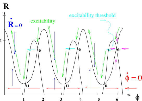
FIG. 1.: Nullclines and fixed points of the forced Ginzburg-Landau equation for $\gamma=\beta=1$, $\mu=0.25$ in the $R,\phi$ plane. Black arrows indicate the dynamical flow along the nullcline $\dot{R}=0$, while grey arrows indicate the dynamical flow along the nullcline $\dot{\Phi}=0$

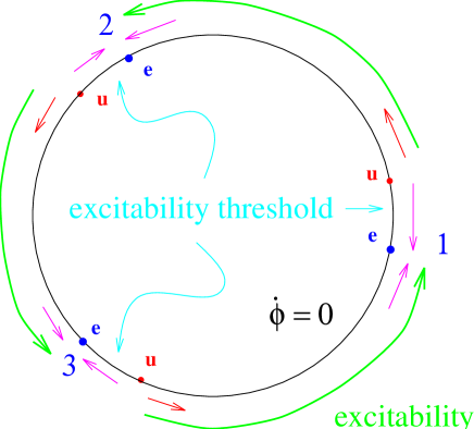
FIG. 2.: Nullcline $\dot{R}=0$ in the complex $A$ plane. Along this nullcline the fixed points $u$ and $e$ are determined by $\dot{\Phi}=0$. Parameter values are $\gamma=\beta=0.01$, $\mu=0.25$. Note that for these parameter values $R_{+}\approx R_{-}$. Arrows indicate the dynamical flow, with long arrows indicating the excitable excursions associated with an heteroclinic trajectory.

FIG. 3.: Uniform solutions of eq. (4) for several values of the forcing parameter $\gamma$. System parameters are $\mu=1$, $\beta=-2.0$ (so $\gamma_{c}=1.57$). Note that for $\gamma<\gamma_{c}$ uniform solutions are of the limit cycle type whereas for $\gamma>\gamma_{c}$ they become fixed points.

FIG. 4.: Plot of the phase field in the excitable regime in 1d. Note the existence of three homogeneous phase states. The arrows indicate the direction of motion of the several fronts. Parameter values are $\mu=1$, $\alpha=2$, $\beta=-0.2$, $\gamma=0.5$.

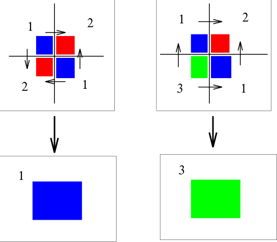
FIG. 5.: Examples of motion of pairs of inclined fronts separating domains with equivalent steady states of the forced Ginzburg-Landau equation for $\gamma>\gamma_{c}$.

$\mu$	$\alpha$	$\beta$	$\gamma_{c}$	Phase approx. valid?	$1+\alpha\beta$	Regime ($\gamma=0$)	Figure
$1.0$	$2.0$	$-0.20$	$0.20$	Yes	$>0$	Frozen states	6, 7
$1.0$	$5.5$	$-0.20$	$0.20$	Yes	$<0$	Frozen states	8
$1.0$	$2.0$	$-0.76$	$0.72$	No	$<0$	Phase turbulence	9
$1.0$	$0.0$	$-1.80$	$1.45$	No	$>0$	Defect turbulence	10, 11

TABLE I.: Parameters of the various cases discussed in section V.

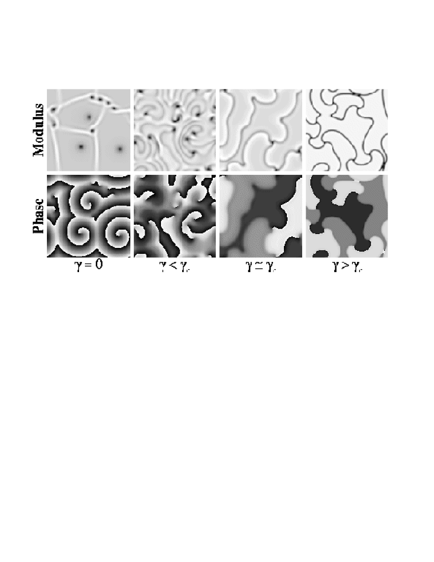
FIG. 6.: Modulus and phase of the complex field $A$ in the cases $\gamma=0$ (no forcing), $\gamma<\gamma_{c}$ (oscillatory), $\gamma\simeq\gamma_{c}$ and $\gamma>\gamma_{c}$ (excitable). Parameter values are $\mu=1$, $\alpha=2$, $\beta=-0.2$ (so that $\gamma_{c}\simeq 0.2$), and $\gamma=0.1\ (0.25)$ for the oscillatory (excitable) case.

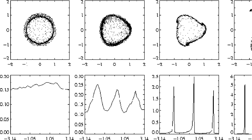
FIG. 7.: Phase portrait (upper row) in the complex plane of the field $A$ and corresponding histograms (lower row) of the phase field. Plots have been made from the snapshots of figure 6.

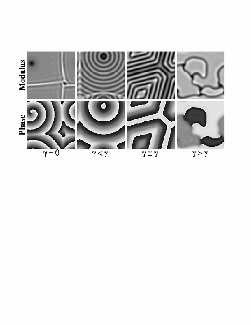
FIG. 8.: Same as in figure 6. Parameter values are $\mu=1$, $\alpha=5.5$, $\beta=-0.2$ ($\gamma_{c}\simeq 0.2$), and $\gamma=0.1\ (0.25)$ for the oscillatory (excitable) case.

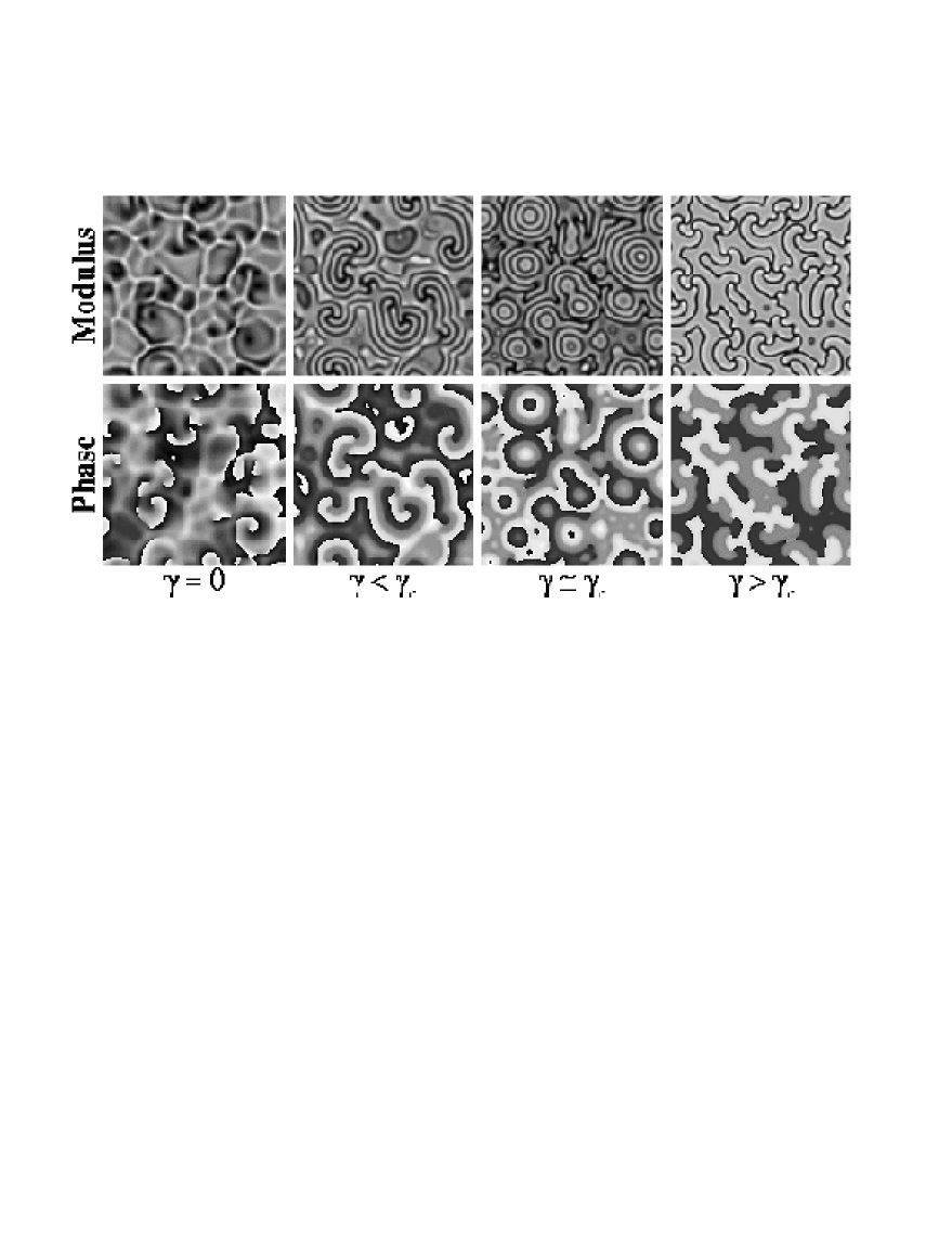
FIG. 9.: Same as in figure 6. Parameter values are $\mu=1$, $\alpha=2$, $\beta=-0.76$ ($\gamma_{c}\simeq 0.72$), and $\gamma=0.5\ (1.5)$ for the oscillatory (excitable) case.

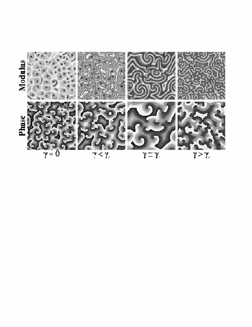
FIG. 10.: Same as in figure 6. Parameter values are $\mu=1$, $\alpha=0$, $\beta=-1.8$ ($\gamma_{c}\simeq 1.45$), and $\gamma=1\ (1.6)$ for the oscillatory (excitable) case.

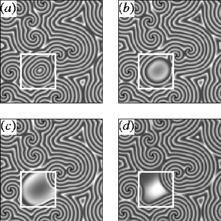
FIG. 11.: Snapshots of the modulus of the field in a regime of parameters where an oscillatory instability at zero wave number occurs. The square encloses an oscillating region. Time increases when going from (a) to (d).

REFERENCES

- [1] J. Guckenheimer and P. Holmes in Nonlinear Oscillations, Dynamical Systems and Bifurcations of Vector Fields, Springer-Verlag, New York (1983).
- [2] H. Bai-Lin in Chaos, World Scientific, Singapore (1983).
- [3] P. Bak and J. von Boehm, Phys. Rev. B 21, 5297 (1980).
- [4] L. N. Bulaevskii and D. I. Khomskii, Sov. Phys. JETP 47, 971 (1978).
- [5] M. Lowe and J. P. Gollub, Phys. Rev. A 31, 3893 (1985).
- [6] T. C. Lubensky and K. Ingersent in Patterns, Defects and Microstructures in Nonequilibrium Systems, NATO ASI Series E121, D. Walgraef ed., Martinus Nijhoff, Dordrecht (1987), p. 48.
- [7] P. Coullet, Phys. Rev. Lett. 56, 724 (1986).
- [8] H. Riecke, J. D. Crawford, and E. Knobloch, Phys. Rev. Lett. 61, 1942 (1988).
- [9] D. Walgraef, Europhys. Lett. 7, 485 (1988).
- [10] I. Rehberg, S. Rasenat, J. Fineberg, M. De La Torre Juárez, and V. Steinberg, Phys. Rev. Lett. 61, 2449 (1988).
- [11] P. Coullet and D. Walgraef, Europhys. Lett. 10, 525 (1989).
- [12] R. Montagne, E. Hernández–García and M. San Miguel, Physica D 96, 47 (1996); M. San Miguel and R. Toral, Stochastic Effects in Physical Systems, in Instabilities and Nonequilibrium Structures VI, Eds. E. Tirapegui, J. Martínez and R. Tiemann, Kluwer Academic Publishers, 35 (2000).
- [13] P. Coullet and K. Emilsson, Physica D 61, 119 (1992).
- [14] C. Elphick, A. Hagberg, and E. Meron, Phys. Rev. Lett. 80, 5007 (1998); Phys. Rev. E 59, 5285 (1999).
- [15] V. Petrov, Q. Ouyang, and H. L. Swinney, Nature 388, 655 (1997).
- [16] A. L. Lin, V. Petrov, H. L. Swinney, A. Ardelea, and G. F. Carey,Resonant pattern formation in a spatially extended chemical system, in Pattern Formation in Continuous and Coupled Systems”, volume 115 in the IMA Volumes in Mathematics and its Applications, edited by M. Golubitsky, D. Luss, and S. H. Strogatz (Springer-Verlag, 1999), pp. 193-202.
- [17] A. L. Lin, M. Bertram, K. Martinez, H. L. Swinney, A. Ardelea, and G. F. Carey, Phys. Rev. Lett. 84, 4240 (2000).
- [18] A. L. Lin, A. Hagberg, A. Ardela, M. Bertram, H. L. Swinney, and E. Meron, Four-phase patterns in forced oscillatory systems, nlin/0003047.
- [19] J. M. Gambaudo, J. Diff. Eq. 57, 172 (1985).
- [20] A. Lin and H. L. Swinney (unpublished).
- [21] F. H. Busse and K. E. Heikes, Science 208, 173 (1980).
- [22] Y. Tu and M. C. Cross, Phys. Rev. Lett. 69, 2515 (1992).
- [23] R. Gallego, M. San Miguel, and R. Toral, Phys. Rev. E 58, 3125 (1998); R. Gallego, M. San Miguel, and R. Toral, Physica A 257, 207 (1998).
- [24] D. Walgraef, Spatio-Temporal Pattern Formation, Springer-Verlag, New York, 1996.
- [25] A. A. Andronov, A. A. Vitt, and S. E. Khaikin, Theory of Oscillators, Pergamon Press, Oxford (1996).
- [26] S. C. Mueller, P. Coullet, and D. Walgraef, Chaos 4, 439 (1994).
- [27] P. S. Hagan, SIAM J. Appl. Math. 42, 762 (1982).
- [28] T. Yamada and Y. Kuramoto, Prog. Theor. Phys. 55, 2035 (1976).
- [29] S. Rica and E. Tirapegui, Physica D 48, 396 (1991).
- [30] L. Kramer, I. Aranson, and A. Weber, Physica D 53, 376 (1991).
- [31] L. M. Pismen and A. A. Nepomnyashchy, Physica D 54, 183 (1992).
- [32] P. Coullet, L. Gil, and J. Lega, Phys. Rev. Lett. 62, 1619 (1989).
- [33] H. Chaté and P. Manneville, Physica A 224, 348 (1996).