Generalizations of the Störmer Problem for
Dust Grain Orbits

H.R. Dullin
Department of Mathematical Sciences, Loughborough University
Leicestershire, LE11 3TU, United Kingdom

M. Horányi and J. E. Howard
Laboratory for Atmospheric and Space Plasmas
University of Colorado, Boulder, CO 80309-0392

Abstract: We consider the generalized Störmer Problem that includes the electromagnetic and gravitational forces on a charged dust grain near a planet. For dust grains a typical charge to mass ratio is such that neither force can be neglected. Including the gravitational force gives rise to stable circular orbits that encircle that plane entirely above/below the equatorial plane. The effects of the different forces are discussed in detail. A modified 3rd Kepler’s law is found and analyzed for dust grains.

PACS: 96.30.Wr, 45.50.Jf, 96.35.Kx

Keywords: Stormer Problem, Dust Grains, Halo Orbits, Stability

1 Introduction

One of the early milestones of space physics was Störmer’s theoretical analysis of charged particle motion in a purely magnetic dipole field [1,2]. This seminal study provided the basic physical framework that led to the understanding of the radiation belts surrounding the Earth and other magnetized planets. The radiation belts are now known to be composed of individual ions and electrons whose motion is often well described by magnetic forces alone. These classical results are also relevant to the dynamics of charged dust grains in planetary magnetospheres. However, the much smaller charge-to-mass ratios produce a more complex dynamics, as planetary gravity and the corotational electric field must also be taken into account [3-6].

In a series of recent papers [7-10] equilibrium and stability conditions were derived for charged dust grains orbiting about Saturn. These orbits can be highly non-Keplerian and include both positively and negatively charged grains, in prograde or retrograde orbits. The first article was restricted to equatorial orbits, while the second treated nonequatorial “halo” orbits, i.e. orbits which do not cross the equatorial plane. Both assumed Keplerian gravity, an ideal aligned and centered magnetic dipole rotating with the planet, and concomitant corotational electric field. The third paper dealt with the effects of planetary oblateness ($J_{2}$), magnetic quadrupole field, and radiation pressure. While the first two forces were found to have a negligible effect on particle confinement, the effects of radiation pressure could be large for distant orbits. Interestingly, $J_{2}$ and radiation pressure can act synergistically to select out one-micron grains in the E-Ring [11]. The final paper in this series allowed the surface potential of a grain, and hence its charge, to adjust to local photoelectric and magnetospheric charging currents. It was concluded that stable halo orbits were mostly likely to be composed of rather small $(\approx 100nm)$ positively charged grains in retrograde orbits. A dust grain “road map” was drawn for the Cassini spacecraft now en route to Saturn, showing where to expect dust grains of a given composition and radius.

This paper presents a more comprehensive treatment of dust grain dynamics, but under the simplified assumptions of Keplerian gravity, pure dipole magnetic field, and no radiation pressure. Some of the results were already presented in the letters [7,8], here we fill in the details of the necessary calculation and also present new results. Our goals are a mathematically rigorous yet simplified derivation of equilibrium and stability conditions which highlights the relative importance of the several different forces acting on an individual grain.

As is well known, there are no stable equilibrium circular orbits for the pure Störmer problem of charged particle motion in a pure dipole magnetic field. It is the addition of planetary gravity and spin that gives rise to stable families of equatorial and nonequatorial orbits. We begin with a general discussion of charged particle motion in axisymmetric geometry, which is then specialized to the motion of charged grains in a planetary magnetosphere. Equilibrium conditions are derived first for equatorial orbits, then for halo orbits. Next we take up the issue of stability for each family of equilibrium orbits. Results are presented for four distinct problems: the Classical Störmer Problem (CSP) in which a charged particle moves in a pure dipole magnetic field, the Rotational Störmer Problem (RSP), with the electric field due to planetary rotation included, the Gravitational Störmer Problem (GSP), with Keplerian gravity included but not the corotational electric field, and the full system (RGSP) including both fields. For each case one must also consider each charge sign in prograde or retrograde orbits. Our results may be summarized as follows:

CSP:

As is well known, no stable circular orbits, equatorial or nonequatorial exist. However, under adiabatic conditions important families of guiding center orbits confined to a potential trough called the Thalweg exist. Such trajectories lie outside the scope of the present paper.

RSP:

Stable equatorial equilibria exist for both charge signs. There are no halo orbits.

GSP:

Stable equatorial equilibria exist for both charge signs. Positive halos are retrograde and negative halos are prograde. Both types are stable wherever they exist.

RGSP:

Stable equatorial equilibria exist for both charge signs. There is a range of positive charge-to-mass ratios without stable equatorial equilibria. Negative halos are prograde, while positive halos can be pro- or retrograde. For stability the frequency must be sufficiently different from twice the rotation rate of the planet.

Therefore halo orbits do exist with and without the corotational electric field. However, the corotational electric field is required in order to sustain stable positive prograde halos.

2 Charged particle dynamics in axisymmetric geometry

The equations of motion of a particle of mass $m$ and charge $q$ in ${\mathbb{R}}^{3}$, ${\bf r}=(x,y,z)^{t}$, are

$$m\ddot{\bf r}=\frac{q}{c}{\bf B}\times{\dot{\bf r}}-\nabla U({\bf r})\,,$$

where the potential $U(\bf r)$ generates the forces of gravity and perhaps corotational electric field. Denote by $R$ a rotation around the $z$ axis and assume that the magnetic field ${\bf B}$ and the potential $U$ are symmetric with respect to this rotation:

$${\bf B}(R{\bf r})=R{\bf B(r)},\quad\nabla U(R{\bf r})=R\nabla U({\bf r})\,.$$

In particular this is true for the field ${\bf B=\nabla\times A}$ of a centered magnetic dipole of strength ${\cal M}$ and dipole axis the $z$ axis, for which the vector potential is, in the Coulomb gauge,

$${\bf A(r)}={\cal M}(y,-x,0)^{t}/r^{3},\quad r^{2}=x^{2}+y^{2}+z^{2}\,.$$

The equations of motion can be transformed to a rotating coordinate system using a rotation matrix $R$ corresponding to the angular velocity ${\bf\Omega}=(0,0,\Omega)^{t}$ which rotates around the $z$-axis with with angular speed $\Omega$. For given angular velocity $\bf\Omega$ the $z$ axis is chosen in the same direction, so that $\Omega$ is positive. Note that the magnetic moment $\cal M$ can be positive or negative. Direct differentiation then gives

$${\bf r}=R{\bf q},\quad\dot{\bf r}=R({\bf\dot{q}+\Omega\times q}),\quad\ddot{\bf r}=R({\bf\ddot{q}}+2{\bf\Omega\times\dot{q}+\Omega\times(\Omega\times q)})\,.$$

so that

$$m\ddot{\bf q}=(\frac{q}{c}{\bf B}-2m{\bf\Omega})\times\dot{\bf q}-m{\bf\Omega\times(\Omega\times q)}+\frac{q}{c}{\bf B\times(\Omega\times q)}-\nabla U({\bf q})\,,$$

where $-2m{\bf\Omega}\times\dot{\bf q}$ is the Coriolis force and $-m{\bf\Omega\times(\Omega\times q)}$ is the centrifugal force. Following the standard argument the term $\frac{q}{c}{\bf B\times(\Omega\times q)}$ is not present in a frame rotating with the planet, because there is no additional electric field. Therefore there must be the same term in $\nabla U$ in order to cancel it. In particular we model the situation inside the corotating plasma, for which this assumptions is reasonable. Transforming back to the rest frame this addition to the potential gives the corotational electric field observed in the rest frame. The corresponding potential is obtained from

$${\bf E}=\frac{q}{c}{\bf B\times(\Omega\times r)}=\gamma\Omega\nabla\Psi,\quad\Psi=\frac{x^{2}+y^{2}}{r^{3}}\,,$$

where $\gamma=q{\cal M}/c$. The electric field ${\bf E}$ is unipolar, i.e. its curl is zero, and therefore it is not induced by a changing magnetic field. Moreover, it is perpendicular to the magnetic field, ${\bf E\cdot B}=0$. The divergence of this field is not zero; instead we find $\nabla\cdot{\bf E}=2\gamma\Omega(2z^{2}-x^{2}-y^{2})/r^{5}$, so that there is a space charge distribution originating from the rotation of the plasma.

In an inertial frame the potential now reads

$$U({\bf r})=-\sigma_{g}\frac{\mu m}{r}+\sigma_{r}\gamma\Omega\Psi\,,$$

where the parameters $\sigma_{g}$ and $\sigma_{r}$ serve as markers of the gravitational and electric forces in order to track the origin of the various terms after scaling away excess parameters. Usually we consider $\sigma_{r}=\sigma_{g}=1$; the classical Störmer problem [1] has $\sigma_{r}=\sigma_{g}=0$. The case $\sigma_{r}=0$ and $\sigma_{g}=1$ has also been studied by Störmer [1,2]; we shall refer to it as the “Gravitational Störmer Problem.” While it is simpler than our case, it will turn out that the most important physical effects can already be seen in this subcase. Another interesting special case is $\sigma_{g}=0$ and $\sigma_{r}=1$. This takes into account the effect of the electric field in the rotating plasma, but the particle is still massless. We call this case the “Rotational Störmer Problem.” It will turn out that in this case halo orbits do not exist.

The Hamiltonian of the above equations of motion is

$$H=\frac{1}{2m}\left({\bf p}-\frac{q}{c}{\bf A(r)}\right)^{2}+U({\bf r})\,.$$ (1)

Owing to the symmetry of the problem the $z$ axis is an invariant set. Because it is singular in coordinates adapted to the symmetry of the problem it is best analyzed in cartesian coordinates. The magnetic field is parallel to this axis, so that for motion on this axis there is no Lorentz force. For initial conditions in the set $x=y=p_{x}=p_{y}=0$ the equations of motion in cartesian coordinates show that the derivatives of $x,y,p_{x},p_{y}$ are zero; hence it is an invariant set, on which the Hamiltonian is purely gravitational, $H_{z}=p_{z}^{2}/2m-\mu m/z$. Depending on the initial conditions in the invariant set a particle either collides with the planet or escapes to infinity; there are no stationary points on this axis.

In cylindrical coordinates $(\rho=\sqrt{x^{2}+y^{2}},\phi=\arctan(y,x),z)$ $H$ becomes

$$H=\frac{1}{2m}\left(p_{\rho}^{2}+p_{z}^{2}+\frac{1}{\rho^{2}}(p_{\phi}-\gamma\Psi)^{2}\right)-\sigma_{g}\frac{\mu m}{r}+\sigma_{r}\gamma\Omega\Psi\,,$$ (2)

with the dipole stream function $\Psi=\rho^{2}/r^{3}$. For systems with $S^{1}$ symmetry a stream function $\Psi$ independent of $\phi$ can always be introduced. The corresponding vector potential is $(\sin\phi,-\cos\phi,0)^{t}\Psi/\rho$, the magnetic field is $(x\Psi_{z},y\Psi_{z},-\rho\Psi_{\rho})^{t}/\rho^{2}$, and the electric field is $\Omega(x\Psi_{\rho},y\Psi_{\rho},\rho\Psi_{z})^{t}/\rho$.

We may distinguish three types of constants in the problem:

• Parameters describing the planet’s mass $\mu=GM$ and spin rate $\Omega$. They are the most fixed parameters.

• Parameters describing the dust particle’s mass $m$ and charge, measured by $\gamma=q{\cal M}/c$.

• The angular momentum $p_{\phi}$ and total energy $h=H$ are constants of the motion determined by the initial conditions. Fixing both $h$ and $p_{\phi}$ defines a region of possible motion in configuration space.

We now introduce a convenient scaling to reduce the number of parameters. Time is measured by the inverse frequency of the planetary spin rate $\Omega$. Distances are measured in terms of the radius of the Keplerian synchronous orbit

$$R=(\mu/\Omega^{2})^{1/3}\,$$

while mass is measured in units of the particle mass $m$. The scaled Hamiltonian is then

$$\hat{H}=\frac{1}{2}\left(\hat{p}_{\rho}^{2}+\hat{p}_{z}^{2}+\left(\frac{\hat{p}}{\hat{\rho}}-\delta\frac{\hat{\rho}}{\hat{r}^{3}}\right)^{2}\right)-\frac{\sigma_{g}}{\hat{r}}+\sigma_{r}\delta\frac{\hat{\rho}^{2}}{\hat{r}^{3}}\,,$$ (3)

where the variables with hat are measured in the new scale. From now on we drop all hats. The essential dimensionless parameters are

$$p=p_{\phi}\frac{R\delta}{\gamma}\qquad\text{and}\qquad\delta=\frac{\Omega\gamma}{m\mu}=\frac{q}{m}\frac{\cal M}{c}\frac{\Omega}{GM}={{\omega_{c}\Omega}\over{\omega_{k}^{2}}}$$

where $\omega_{c}=qB_{0}/mc$ is the cyclotron frequency, $B_{0}$ is the planetary magnetic field on the equator, $\omega_{k}=\sqrt{GM/R_{s}^{3}}$ is the Kepler frequency, with $R_{s}$ the planetary radius, and the parameter $p$ is just the angular momentum $p_{\phi}$ measured in the new units. The single parameter for the dust grain is $\delta$, which is essentially the charge-to-mass ratio. Recall that the $z$ axis is oriented so that $\Omega>0$. In the following we will loosely talk about positive/negative charge when we mean positive/negative $\delta$. This correspondence is correct if the magnetic dipole moment $\cal M$ is positive, i.e. the spin and the field are aligned. This is true for Saturn, the main application that we have in mind. Our results are valid in both cases.

3 Equilibria

3.1 Equatorial Orbits

Here we shall find it advantageous to work in spherical coordinates $(r=\sqrt{\rho^{2}+z^{2}},\theta=\arccos(z/r),\phi)$, rather than the cylindrical coordinates of Ref [7,8]. The Hamiltonian becomes

$$H=\frac{1}{2}\left(p_{r}^{2}+\frac{p_{\theta}^{2}}{r^{2}}\right)+U_{\rm eff}\,,$$ (4)

where the effective potential $U_{\rm eff}$ is the part of the Hamiltonian independent of the non-constant momenta $p_{r}$ and $p_{\theta}$:

$$U_{\rm eff}(r,\theta,p)=\frac{(pr-\delta\sin^{2}\theta)^{2}}{2r^{4}\sin^{2}\theta}-\frac{\sigma_{g}-\sigma_{r}\delta\sin^{2}\theta}{r}\,.$$ (5)

The equations of motion are then

$$\dot{r}=p_{r},\quad\dot{\theta}=p_{\theta},\quad\dot{\phi}=\partial_{p}U_{\rm eff},$$ (6)

$$\dot{p}_{r}=-\partial_{r}U_{\rm eff},\quad\dot{p}_{\theta}=-\partial_{\theta}U_{\rm eff},\quad\dot{p}_{\phi}=0\,.$$ (7)

In order to facilitate the calculation of the partial derivatives of $U_{\rm eff}$ we introduce the frequency

$$\omega(r,\theta)=\dot{\phi}=\partial_{p}U_{\rm eff}=\frac{p}{r^{2}\sin^{2}\theta}-\frac{\delta}{r^{3}}\,.$$ (8)

In analyzing circular equilibrium orbits it is preferable to employ $\omega$ rather than $p_{\phi}$ as parameter, as it is the sign of $\omega$ that determines whether the orbit is rotating in the same direction as the planet (prograde) or opposite to it (retrograde). Recall that in the scaled variables frequencies are measured in terms of $\Omega$; hence $\omega=1$ means synchronous motion. From now on we will eliminate $p$ in favour of $\omega=\omega(r,\theta)$ in the potential to get

$$U_{\rm eff}=\frac{1}{2}\omega^{2}r^{2}\sin^{2}\theta-\frac{\sigma_{g}}{r}+\frac{\sigma_{r}\delta\sin^{2}\theta}{r}\,.$$ (9)

It is important to notice that when calculating derivatives of $U_{\rm eff}$ with respect to $r$ and $\theta$ we have to treat $\omega$ as a function of $r$ and $\theta$. The derivatives of $\omega$ (re-expressed in terms of $\omega$) are

$$\partial_{r}\omega = -2\frac{\omega}{r}+\frac{\delta}{r^{4}}$$

$$\partial_{\theta}\omega = -2\cot\theta\left(\omega+\frac{\delta}{r^{3}}\right)\,,$$

so that

$$\partial_{r}U_{\rm eff} = -\omega^{2}r\sin^{2}\theta+\frac{1}{r^{2}}(\delta(\omega-\sigma_{r})\sin^{2}\theta+\sigma_{g})$$ (10)

$$\partial_{\theta}U_{\rm eff} = -\frac{1}{r}\cos\theta\sin\theta(\omega^{2}r^{3}+2\omega\delta-2\sigma_{r}\delta)\,.$$ (11)

If all partial derivatives with respect to $r$, $\theta$, and $p$ are zero there is no motion at all. The latter is just $\omega$, which we set to zero. Then (11) requires $\theta=\pi/2$. The other possibility $\theta=0,\pi$ is the coordinate singularity, and it has already been treated using $H_{z}$. The uncharged case $\delta=0$ is not of interest here. For $\theta=\pi/2$ and $\omega=0$ (10) reduces to $\sigma_{g}=\sigma_{r}\delta$. Therefore particles at rest can occur anywhere in the equatorial plane but only when $\delta=\sigma_{g}/\sigma_{r}$. Therefore $\delta=1$ can be considered as the case where electrical and gravitational forces are balanced. In the classical Störmer problem $\sigma_{r}=\sigma_{g}=0$ both equations are automatically satisfied once $\omega=0$. In this case we can place a particle at rest anywhere in space; since there is no potential there are no forces if there is no motion. In any case it is true that for these trivial solutions at rest the angular momentum $p$ is nonzero; from $\omega=0$ and (8) we find $p=\delta/r$. The energy is zero for all these equilibrium points.

The system has a discrete symmetry: the equations of motion are invariant under the map $(\theta,p_{\theta})\to(\pi-\theta,-p_{\theta})$. The set that is invariant under this map is the equatorial plane with no transverse momentum, $(\theta,p_{\theta})=(\pi/2,0)$. As always this is also an invariant set for the dynamics. The physical reason for this is that ${\bf B(r)}$ is parallel to the $z$ axis if ${\bf r}=(x,y,0)$, so that for motion within the equatorial plane there is a Lorentz force, however, with direction in the plane. Moreover, ${\bf E(r)}$ is perpendicular to ${\bf B(r)}$, and therefore ${\bf E(r)}$ lies in the equatorial plane if ${\bf r}=(x,y,0)$. The Hamiltonian restricted to the equatorial plane reads

$$H_{xy}=\frac{1}{2}\left(p_{r}^{2}+\frac{1}{r^{2}}\left(p-\frac{\delta}{r}\right)^{2}\right)-\frac{\sigma_{g}-\sigma_{r}\delta}{r}\,.$$

This is an integrable system with one effective degree of freedom that can be solved in terms of elliptic functions. The effective potential in the equatorial plane is

$$U_{xy}(r)=\frac{1}{2}\left(\frac{p}{r}-\frac{\delta}{r^{2}}\right)^{2}-\frac{\sigma_{g}-\sigma_{r}\delta}{r}=\frac{1}{2}\omega^{2}r^{2}-\frac{\sigma_{g}-\sigma_{r}\delta}{r}\,.$$

The minima $r_{e}$ of $U_{xy}(r)$ correspond to circular orbits in the equatorial plane because the right hand sides of all the equations of motion except $\dot{\phi}=\omega$ are zero. The calculation of critical points of $U_{xy}(r)$ leads to the solution of a cubic polynomial in $r$ given by $r^{2}\partial_{r}U_{xy}$. If instead we eliminate $p$ in favour of $\omega$ we obtain a much simpler polynomial

$$P(r,\omega)=\omega^{2}r^{3}-\omega\delta+\sigma_{r}\delta-\sigma_{g}\,.$$ (12)

Figure 1: Existence of equatorial orbits

Solving $P=0$ for $r$ yields a generalization of Kepler’s 3rd law for equatorial orbits:

$$r_{e}(\omega)^{3}=\frac{\sigma_{g}+\delta(\omega-\sigma_{r})}{\omega^{2}}\,.$$ (13)

which for $\delta\to 0$ reduces to the ordinary Kepler’s law. The corresponding angular momentum $p$ can be calculated from (8) and is $p_{e}=\omega r_{e}^{2}-\delta/r_{e}$. The radius $r_{e}$ is positive if

$$\omega\leq\sigma_{r}-\frac{\sigma_{g}}{\delta} \delta\leq 0,\qquad\text{or}$$ and (14)

$$\omega\geq\sigma_{r}-\frac{\sigma_{g}}{\delta} \delta\geq 0\,.$$ and (15)

For negative $\delta$ there are always pro- and retrograde orbits. For positive $\delta$ this is only true for $\delta<\sigma_{g}/\sigma_{r}$, while for $\delta>\sigma_{g}/\sigma_{r}$ all orbits are prograde. In Fig. 1 the possible combinations of $\omega$ and $\delta$ for which circular equatorial orbits exist are shaded grey. The horizontal asymptotes have $\omega=\sigma_{r}$. The hyperboloidal boundaries and the limit $\omega\to\infty$ correspond to zero radius. In the Störmer case $\sigma_{r}=\sigma_{g}=0$ all equatorial circular orbits of negatively charged particles ($\delta<0$) are retrograde ($\omega<0$), while positively charged particles have prograde orbits. The gravitational and/or electric field perturbations create small regions of the opposite behaviour for some $\delta$. In addition some motions for large positive $\delta$ and small positive $\omega$ are made impossible by switching on the additional fields.

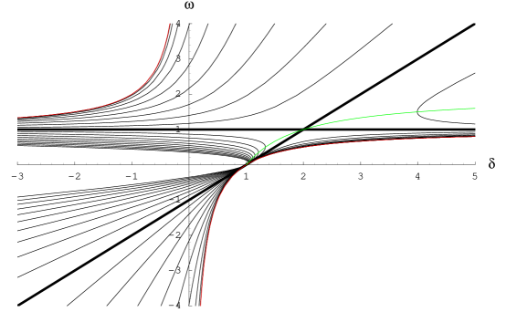
Figure 2: Curves of constant radius $r=0.1i$, $i=1,\dots,20$ for equatorial orbits. The thick lines have $r=1$.

The equation for equatorial orbits, $P=0$, can be solved for $\delta$ in order to give $\delta$ as a function of $\omega$ for given $r$:

$$\delta=\frac{r^{3}\omega^{2}-\sigma_{g}}{\omega-\sigma_{r}}\,.$$

These curves are shown in Fig. 2 and 3. Note the two straight lines with $r=1$, which in our scaling is the radius of the synchronous orbit in the Kepler problem. The horizontal one corresponds to the synchronous orbits ($\omega=1$) which exist for any $\delta$. Hence the synchronous Kepler orbit is not affected by the addition of both fields. This is not true for the three Störmer cases, see below. Another prominent feature is the point $(\delta,\omega)=(1,0)$, which is intersected by hyperbolas with all $r$. It corresponds to the equilibrium points discussed above.

       

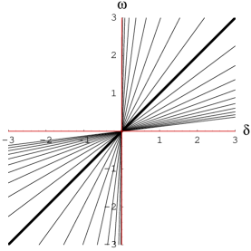
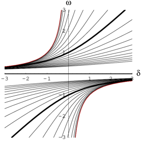
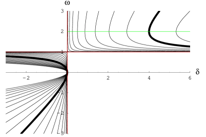
Figure 3: Curves of constant radius for equatorial orbits of the a) classical ($\sigma_{r}=\sigma_{g}=0$), b) gravitational ($\sigma_{r}=0,\sigma_{g}=1$), and c) rotational ($\sigma_{r}=1,\sigma_{g}=0$) Störmer problem. Thick lines have $r=1$.

Let us briefly discuss the corresponding diagrams for the three Störmer cases shown in Fig. 3. In the classical case $\omega$ and $\delta$ are proportional. Small slope means large $r$. The relation breaks down for the line $\omega=0$ for which all radii are possible. There are only two other types of equatorial orbits: positively charged prograde and negatively charged retrograde. In the gravitational Störmer case the relation between $\omega$ and $\delta$ is quite similar, but now there are also small regions of the two types of motions: positively charged retrograde and negatively charged prograde. In the rotating Störmer case the positive retrograde orbits have disappeared again. The main new feature is the appearance of orbits of small negative charge with small $\omega$ and small radius.

3.2 Halo Orbits

Our goal is the calculation of periodic orbits that encircle the planet in a plane parallel to the equatorial plane but entirely above/below it. Circular orbits correspond to critical points of $U_{\rm eff}$, i.e. points $(r_{0},\theta_{0})$ at which both derivatives of $U_{\rm eff}$ vanish. This is so because at $(r,\theta,p_{r},p_{\theta})=(r_{0},\theta_{0},0,0)$ the right hand sides of Hamilton’s equations are zero, except for $\dot{\phi}$. They are given by the minima of $U_{\rm eff}$. Their stability will be calculated in the next section.

Circular orbits are given by the solution of $\partial_{r}U=0$ and $\partial_{\theta}U=0$ for arbitrary $\omega$, see (10,11). The second equation has the solution $\theta=\pi/2$, which gives the equatorial orbits we already analyzed. Also the solutions with $\theta=0,\pi$ have already been described using the reduced Hamiltonian $H_{z}$. The remaining solutions are given by $Q=0$ with

$$Q(r,\omega)=\omega^{2}r^{3}+2\omega\delta-2\sigma_{r}\delta\,,$$ (16)

which describe the nonequatorial (or halo) orbits. The equation $Q=0$ can be solved for $r^{3}$, which can then be eliminated from (11) resulting in an angular equation $A=0$ with

$$A(\theta,\omega)=\sigma_{g}+3\delta(\omega-\sigma_{r})\sin^{2}\theta\,.$$ (17)

The functions $Q$ and $A$ completely describe the halo orbits. In particular these equations can easily be solved for $r$ and $\theta$, so that all circular orbits are obtained in parametric form, with $\omega$ as a parameter. Explicitly we find

$$r_{h}(\omega)^{3} = 2\delta\frac{\sigma_{r}-\omega}{\omega^{2}}$$ (18)

$$\sin^{2}\theta_{h}(\omega) = \frac{\sigma_{g}}{3\delta(\sigma_{r}-\omega)}\,.$$ (19)

grains [4]. The second equation clearly shows that without the gravitational forces ($\sigma_{g}=0$) there are no halo orbits. In particular in the classical Störmer problem there are no halo orbits (except for the trivial equilibrium points discussed above). Adding the electric field alone there still are no halo orbits. In both equations it is obvious that the electric field merely shifts the frequency $\omega$ of circular halo orbits. We conclude that the electric field is not essential for the existence of halo orbits.

Figure 4: Existence of halo orbits

For halo orbits the essential condition for their existence is that $\sin^{2}\theta\leq 1$, which implies

$$\omega\geq\sigma_{r}-\frac{\sigma_{g}}{3\delta} \delta\leq 0,\qquad\text{or}$$ and (20)

$$\omega\leq\sigma_{r}-\frac{\sigma_{g}}{3\delta} \delta\geq 0\,.$$ and (21)

These conditions automatically imply that the corresponding radius $r_{h}$ is positive. Note that the ordering of the $\omega$ inequalities is reversed compared with the equatorial case (14,15). Hence for negative charge only prograde orbits exist while for small positive charge only retrograde orbits exist. Only if $\sigma_{r}\not=0$ and for $\delta>\sigma_{g}/3\sigma_{r}$ can both types of orbits exist. The electric field does make a difference for the existence of synchronous halo orbits: If $\sigma_{r}=1$ then $\omega=1$ is impossible for finite $\delta$. If $\sigma_{r}=0$ synchronous halo orbits exist for $\delta<-\sigma_{g}/3$. Note that $\omega=\sigma_{r}$ (in particular a synchronous orbit if $\sigma_{r}=1$) is impossible for finite $\delta$. Without the electric field there do exist synchronous halo orbits with negative charge. In order for $(q/c){\bf B}\times\dot{\bf r}$ to balance gravitation for positive charge we have to reverse $\dot{\bf r}$, hence $\omega=-1$.

To get an overview of all possible halo orbits we plot curves of constant $r$ and $\theta$ in the $\delta$-$\omega$ plane. The family of curves of constant radius is given by

$$\delta=\frac{r^{3}\omega^{2}}{2(\sigma_{r}-\omega)}.$$

The family of curves of constant azimuth $\theta$ is given by

$$\delta=\frac{\sigma_{g}}{3(\sigma_{r}-\omega)\sin^{2}\theta}.$$

Both families are shown in Fig. 5 for $\sigma_{r}=\sigma_{g}=1$ and in Fig. 6 for the Störmer problem with gravitation.

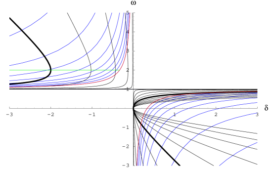
Figure 5: Curves of constant $r$ and $\theta$ for halo orbits. Thick lines have $r=1$. $r=0.2i$, $\sin\theta=0.1i$, $i=1,\dots,10$

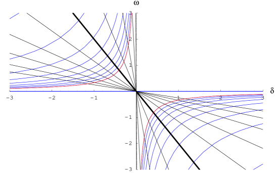
Figure 6: Curves of constant $r$ and $\theta$ for halo orbits in the gravitational Störmer problem. Thick lines have $r=1$. $r=0.2i$, $\sin\theta=0.1i$, $i=1,\dots,10$

The regions of existence in the $\delta$-$\omega$-plane for equatorial and halo orbits only overlap in a small region bounded by hyperbolae. They are in a sense connected at the hyperboloidal boundary of the halo orbits, because in the next section we will find that this line marks a pitchfork bifurcation of an equatorial orbit changing its stability and creating halo orbits.

4 Stability

In Ref [7-8] explicit stability boundaries for both equatorial and halo orbits were calculated. Here we obtain these boundaries more directly using the fact that all circular orbits may be parameterized by $\omega$. A circular orbit is stable if it corresponds to a local minimum of $U$, for which we need the second derivatives of $U$. Using the chain rule gives

$$\partial_{r}^{2}U = \left(3\,{\omega}^{2}-2\delta{\frac{3\,\omega-\sigma_{r}}{{r}^{3}}}+{\frac{{\delta}^{2}}{{r}^{6}}}\right)\sin^{2}\theta-\frac{2\sigma_{g}}{r^{3}}$$

$$\partial_{\theta}^{2}U = \left(2\,{r}^{2}{\omega}^{2}+4\delta{\frac{\omega+\sigma_{r}}{r}}+4\,{\frac{{\delta}^{2}}{{r}^{4}}}\right)\cos^{2}\theta+{r}^{2}{\omega}^{2}+2\delta{\frac{\omega-\sigma_{r}}{r}}$$

$$\partial_{r}\partial_{\theta}U = 2\,\left(r{\omega}^{2}+\delta{\frac{2\omega-\sigma_{r}}{{r}^{2}}}-{\frac{{\delta}^{2}}{{r}^{5}}}\right)\cos\theta\sin\theta.$$

4.1 Equatorial Orbits

For equatorial orbits we insert $\theta=\pi/2$ and $r=r_{e}(\omega)$ as given above. The mixed derivative vanishes and the other two are

$$\partial_{r}^{2}U|_{e} = -\frac{1}{2}\left(\frac{\omega}{\sigma_{g}+\delta(\omega-\sigma_{r})}\right)^{2}((2\omega\delta-\sigma_{r}\delta+\sigma_{g})^{2}-3(\sigma_{r}\delta-\sigma_{g})^{2})$$

$$\partial_{\theta}^{2}U|_{e} = \sigma_{g}+3\delta(\omega-\sigma_{r})\,.$$

The radial derivative diverges for those $\omega$ that correspond to $r=0$. It vanishes for $\omega=0$; however, the corresponding radius $r_{e}$ is not finite (except for $\delta=\sigma_{g}/\sigma_{r}$, the case of equilibrium points). There are two nontrivial factors that correspond to tangent bifurcations of equatorial orbits with

$$\omega_{e}^{\pm}=\frac{1\pm\sqrt{3}}{2}\left(\sigma_{r}-\frac{\sigma_{g}}{\delta}\right)\,.$$

The vanishing of the second $\theta$ derivative indicates the loss of transverse stability. Because of reflection symmetry $\theta\to-\theta$ this results in a pitchfork bifurcation with

$$\omega_{PF}=\sigma_{r}-\frac{\sigma_{g}}{3\delta}.\qquad$$

All three curves are hyperbolas in the space of $(\delta,\omega)$ shown in Fig. 7. The intersection of the curves $\omega_{PF}$ and $\omega_{e}^{\pm}$ occurs at

$$\delta_{e}^{\pm}=\frac{\sigma_{g}}{\sigma_{r}}\frac{5\pm 2\sqrt{3}}{3}\,.$$

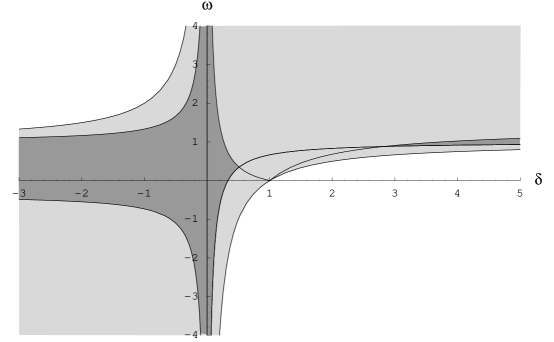
Figure 7: Regions of stability for equatorial orbits are dark. Overlay Fig. 2

Using the above formulas for the second derivatives it is easy to check that stability only holds in the following $\omega$ ranges (compare Fig. 7).

$$\delta<0 : \omega_{e}^{-}<\omega<\omega_{PF}$$

$$0<\delta<\delta_{e}^{-} : \omega_{PF}<\omega<\omega_{e}^{-}$$

$$\delta>\delta_{e}^{+} : \omega_{PF}<\omega<\omega_{e}^{+}\,.$$

For the first two ranges $\omega=0$ is (partially) included, which means that the corresponding family of orbits exists for arbitrary large radius. The radius $r_{e}$ as given by (13) as a function of $\omega$ is a monotone function for most of these orbits except for unstable orbits with $\delta>1$. This gives the additional curve in the diagram. The fact that the radius is not monotonic can already be seen in Fig. 2, where the turning points are marked by a gray line.

   

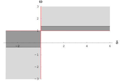
Figure 8: Regions of stability for equatorial orbits of the a) gravitational, and b) rotating Störmer problem are dark. Overlay Fig. 3

For comparison we also show the diagrams in the two nonclassical Störmer cases, see Fig. 8. In the classical Störmer problem with $\sigma_{r}=\sigma_{g}=0$ the derivative $\partial_{r}^{2}U_{\rm eff}|_{e}$ is always negative, hence there are no stable equatorial orbits. In the purely gravitational case stable orbits exist between the pitchfork curve and the tangent bifurcation corresponding to $\omega_{e}^{-}$. The curve $\omega_{e}^{+}$ always is outside the region of existence. In the rotational Störmer problem the pitchfork curves and the existence curves coincide at $\omega=1$. The stable region for $\delta<0$ is between $\omega_{e}^{-}$ and 1, while for $\delta>0$ it is between 1 and $\omega_{e}^{+}$. Comparing these pictures with Fig. 7 one clearly observes that for large $|\delta|$ (i.e. small mass) the systems behaves like the rotating case, while for small $|\delta|$ (i.e. large mass) the behaviour is dominated by gravity and looks like the gravitational case. In the gravitational case there exist stable pro- and retrograde orbits for any $\delta$; the system is symmetric with respect to change of sign of $\omega$ and $\delta$. In the rotational case this symmetry is broken and both pro- and retrograde orbits only exist for negative charge. Trying to interpolate between the large and small $\delta$ behaviour the full system creates an interval $[\delta_{e}^{-},\delta_{e}^{+}]$ of charge-to-mass ratios for which no stable equatorial circular orbits exist.

4.2 Nonequatorial Orbits

In Ref [8] the stability of halo orbits was analyzed by examining the zeros of a quintic in $\rho$. Here we obtain similar results more directly. For nonequatorial orbits the calculation is essentially the same as for their equatorial cousins, except that all three second derivatives are nonzero and we have to calculate the determinant and the trace of the Hessian, which turn out to be

$$\text{det}D^{2}U_{\rm eff}|_{h} = \sigma_{g}\frac{2\omega^{2}(\omega^{2}-4\omega\sigma_{r}+\sigma_{r}^{2})(\sigma_{g}+3\delta(\omega-\sigma_{r}))}{3\delta(\omega-1)^{3}}$$

$$\text{tr}D^{2}U_{\rm eff}|_{h} = -\sigma_{g}\frac{\omega^{2}(13\omega^{2}-16\omega\sigma_{r}+4\sigma_{r}^{2})}{12\delta(\omega-\sigma_{r})^{3}}-\frac{2(\omega-2\sigma_{r})^{2}(\sigma_{g}+3\delta(\omega-\sigma_{r}))}{3r_{h}(\omega)(\omega-\sigma_{r})^{2}}\,.$$

The determinant vanishes in three cases: 1) For $\omega=0$, which again for $\delta\not=1$ does not correspond to finite orbits. Since $\omega$ appears squared there is no change in stability when orbits go through infinity. 2) In the case that the last factor is zero, which reproduces the condition $\omega=\omega_{PF}$. 3) There are two new critical $\omega$ given by the remaining factor as

$$\omega_{h}^{\pm}=\sigma_{r}(2\pm\sqrt{3})\,.$$

These frequency values correspond to tangent bifurcations of halo orbits. The corresponding horizontal lines are also shown in Fig. 7. A pair of stable and unstable orbits is created for this frequency. The lines only extend up to the intersection with the pitch fork curve, which occurs at

$$\delta_{h}^{\pm}=\frac{\sigma_{g}}{\sigma_{r}}\frac{1\pm\sqrt{3}}{6}\,.$$

For $\delta<0$ the upper curve extends up to $\delta_{h}^{-}$, the lower curve is valid for $\delta>0$ and extends from $\delta_{h}^{+}$ to infinity. For $\delta<0$ halo orbits have to be above the pitchfork line. Inserting into the invariants of the Hessian we find that they are stable if they are above $\omega=\omega_{h}^{+}$ and unstable otherwise. In the unstable family there occurs a maximum in radius at $\omega=2$. Otherwise the radius is a monotonous function of $\omega$. For $\delta>0$ stability is reversed: orbits exist below the pitchfork line and are stable if $\omega<\omega_{h}^{-}$. At passage through $\omega=0$ the radius goes to infinity, so that (sufficiently) positively charged retrograde halo orbits exist for all large radii. Hence we obtain the following $\omega$ ranges of existence of stable halo orbits:

$$\delta<\delta_{-} : \omega>\omega_{+}$$

$$\delta_{-}<\delta<0 : \omega>\omega_{PF}$$

$$0<\delta<\delta_{+} : \omega<\omega_{PF}$$

$$\delta>\delta_{+} : \omega<\omega_{-}$$

A simple way to characterize Fig. 9 is to say that halo orbits with frequencies too close to synchronous are unstable. However, the range of unstable frequencies is centered around orbits with $\omega=2$, i.e. orbits that go around twice for one revolution of the planet. Halo orbits with frequencies further away than $\sqrt{3}$ from this are stable. Note that the equatorial orbits behave approximately in the opposite way. For them only orbits with small $\omega$ are stable (except for small $\delta$). This can also be interpreted in terms of the pitchfork bifurcation: once equatorial orbits become too fast, they become unstable and create stable nonequatorial orbits. The corresponding picture for the gravitational Störmer problem is not shown, because it is trivial: in this case every halo orbit is stable, as can be seen from the above expressions for determinant and trace of the Hessian.

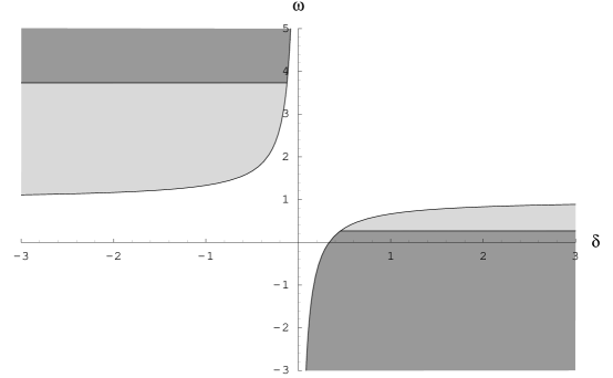
Figure 9: Regions of stable halo orbits are dark. Overlay Fig. 5

5 Stable Halo Orbits in Space

Considering Fig. 5 we see that the curves of constant $r$ and $\theta$ transversely intersect each other in the regions of existence. This means that the transformation from $(r,\theta)$ to $(\delta,\omega)$ is invertible, which we will now show. Instead of transforming to spherical coordinates $(r,\theta)$ we directly transform to cylindrical coordinates. Equations (18) and (19) can be considered as a transformation from $(z,\rho)=(r\cos\theta,r\sin\theta)$ to $(\delta,\omega)$. For each of the four types of orbits distinguished by pro/retrograde and positive/negative charge this is a global transformation because the Jacobian is

$$\det\frac{\partial(z,\rho)}{\partial(\delta,\omega)}=\frac{2}{9\delta\omega^{3}r\sin\theta\cos\theta}\,,$$

which is only singular when $\omega$, $\delta$, $r$, or $\sin 2\theta$ is zero. We already know that the latter two are only zero at the boundaries of the valid region in $(\delta,\omega)$ space. The inverse of the transformation is given by

$$\omega^{2} = \frac{2}{3}\frac{1}{r^{3}\sin^{2}\theta}$$ (22)

$$\delta = \frac{1}{3}\frac{1}{(\sigma_{r}-\omega)\sin^{2}\theta}\,.$$ (23)

The first is a generalization of Kepler’s 3rd law for halo orbits, which surprisingly is independent of the electric field. Compared to the usual law it has effective frequency $\sqrt{3/2}\omega\sin\theta$. From the second equation the corresponding charge to mass ratio can be calculated. These two equations give a precise prediction about what dust particles with what velocities should be observable at a given nonequatorial position $(r,\theta)$.

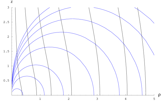
Figure 10: $(\delta,\omega)$ grid in $(\rho,z)$ space for halo orbits in the gravitational Störmer problem. (top left to right $\pm\omega=-2-\sqrt{3},-1,-0.5,-2+\sqrt{3},-0.15,-0.1,-0.08$, bottom $\pm\delta=0.1,0.5,1,2,3,4,5,6$)

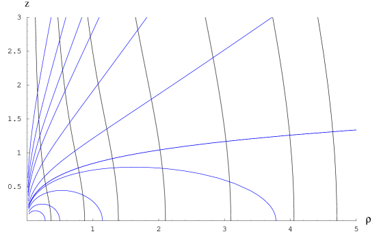
Figure 11: $(\delta,\omega)$ grid in $(\rho,z)$ space for retrograde positive halo orbits. ($\omega$ as in Fig. 10, bottom left to right, then up $\delta=0.05,0.1,0.2,0.3,\frac{1}{3},0.5,1,2,3,5,10$)

   

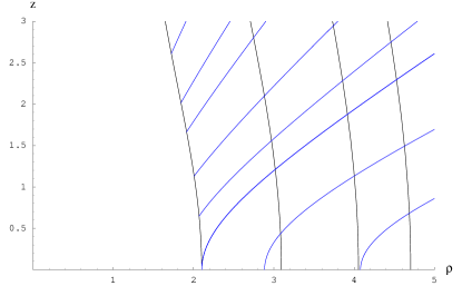
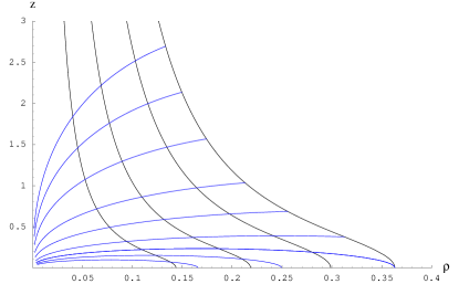
Figure 12: $(\delta,\omega)$ grid in $(\rho,z)$ space for a) prograde positive ($\omega=2-\sqrt{3},0.15,0.1,0.08$, left top to bottom $\delta=1.5,1,0.8,0.6,0.5,(1+\sqrt{3})/6,0.4,0.37$), and b) prograde negative ($\omega=15,8,5,2+\sqrt{3}$, right top to bottom $\delta=-50,-25,-10,-3,-1,-0.3,(1-\sqrt{3})/6,-0.06,-0.03$) halo orbits.

To get an idea about what particles to expect at what position we now plot the curves of constant $\omega$ and $\delta$ on the $\rho$-$z$ plane. The simplest way to do this is to use (18,19) to generate a parametric form of these curves in the $\rho$-$z$ plane:

$$(\rho,z)=(r_{h}\sin\theta_{h},r_{h}\cos\theta_{h}).$$

In the gravitational Störmer case the formulas are

$$(\rho,z)=\left(-\frac{2\delta}{\omega}\right)^{1/3}\left(\sqrt{-1/(3\delta\omega)},\sqrt{1+1/(3\delta\omega)}\right).$$

$\delta$ and $\omega$ have to be restricted to the range of existence, respectively stability, which is the same in the present case. The resulting diagram is shown in Fig. 10. Because there is no coupling to the rotation, prograde and retrograde orbits are the same up to the sign of $\omega$.

For the full system there is an additional region of prograde orbits with $\delta>0$, see Fig. 12. In this case only $(\delta,\omega)$ values from the stable regions are taken to draw the grids. This is the reason for the cutoffs in the prograde case. Note that all the retrograde halo orbits are stable, and therefore for every point in the $(\rho,z)$ plane there exists a unique halo orbit.

Note that all four figures share the same set of lines $\omega={\rm const}$. This is a result of the fact that the generalized 3rd Kepler’s law (22) is independent of $\sigma_{r}$, $\delta$, and independent of the sign of $\omega$. Using the transformation from $(r,\theta)$ to $(\rho,z)$ we can convert this equation into

$$z^{2}=\frac{9}{4}\left(\frac{\omega}{\rho}\right)^{4}-\rho^{2}\,,$$

which is the explicit form of the curves $\omega={\rm const}$ in all four figures. A similar explicit form for the curves $\delta={\rm const}$ can only be obtained with $\sigma_{r}=0$. Then we find $z^{2}=(-\sqrt{6}\delta\rho)^{4/5}-\rho^{2}$. With $\sigma_{r}=1$ the curves in $(\rho,z)$ are described by a polynomial of degree 5 in $z^{2}$ and $\rho^{2}$, so that the above parametric form is the most convenient representation.

Our most important conclusion is that the dependence on $\omega$ is the same with or without the electric field. The distribution of grain sizes as given by the curves of constant $\delta$ is significantly changed. The changes are fairly small for stable retrograde positive orbits. In both cases they exist at any point in space. The prograde negative orbits need quite high angular velocity and only survive close to the $z$ axis. Stable prograde positive halo orbits do not exist at all without an electric field. With the field they need to have a minimal distance of a little more then twice the synchronous radius, and $\delta$ must be around $(1+\sqrt{3})/6$ in order to be able to be close to the planet. It follows that retrograde positive orbits are the most likely candidates for halo orbits.

6 Discussion

We have calculated explicit equilibrium and stability conditions for arbitrary circular orbits in an axisymmetric combination of gravitational, magnetic and corotational electric fields. The equilibrium and stability boundaries were conveniently parametrized by the charge-to-mass ratio $\delta$ and the orbital frequency $\omega$. The individual effects of planetary gravitational field, magnetic field and corotational electric field on the existence and stability of charged dust grain orbits were elucidated.

Our principal result is that halo orbits cannot exist without inclusion of gravitational forces. Without the corotational electric field all halo orbits are stable. The distribution of orbital frequencies of stable halo orbits in space is the same with- and without the corotational electric field, which is the content of a generalized Kepler’s 3rd law (22). The inclusion of the corotational electric field alone does not give halo orbits at all. Adding it to the gravitational field does not have a strong effect on positive retrograde orbits, which are still all stable. It destabilizes negative prograde orbits with small frequencies. Adding the corotational electric field has a surprisingly strong effect on the character of both equatorial and nonequatorial (halo) orbits. In particular, prograde positively charged halos require a corotational electric field for their very existence.

For halo orbits lying several Saturn radii above the equatorial plane the typical surface potential of a dust grain is expected to be around $+5V$, due to the low plasma density there and resultant dominant photoelectric charging. If stable retrograde grains are present, even the very small grains predicted by our theory should be detected by the CDA experiment on board the Cassini orbiter due to arrive in 2004.

References

- [1]
- [2] C. Störmer, The Polar Aurora, (Clarendon Press, Oxford, 1955).
- [3] A. Dragt and J. Finn, J. Geophys. Res. 81, 2327 (1971).
- [4] T. G. Northrop and J. A. Hill, J. Geophys. Res. 87, 6045 (1982).
- [5] D. A. Mendis, J. R. Hill, and H. L. F. Houpis, J. Geophys. Res. 88, A929 (1983).
- [6] D. Hamilton, Icarus 101, 244 (1993).
- [7] R.-L Xu and L. F. Houpis, J. Geophys. Res. 90, 1375 (1985).
- [8] J. E. Howard, M. Horányi, and G. A. Stewart, Phys. Rev. Lett. 83, 3993 (1999).
- [9] J. E. Howard, H. R. Dullin, and M. Horányi, Phys. Rev. Lett. 84, 3993 (2000).
- [10] J. E. Howard and M. Horányi, to be published in Adv. Space. Res..
- [11] J. E. Howard and M. Horányi, to be published in Geophys. Res. Lett..
- [12] M. Horányi, J. A. Burns, and D. P. Hamilton, Icarus 97, 248 (1992).