Freak Waves in Random Oceanic Sea States

Abstract

Freak waves are very large, rare events in a random ocean wave train. Here we study the numerical generation of freak waves in a random sea state characterized by the JONSWAP power spectrum. We assume, to cubic order in nonlinearity, that the wave dynamics are governed by the nonlinear Schroedinger (NLS) equation. We identify two parameters in the power spectrum that control the nonlinear dynamics: the Phillips parameter $\alpha$ and the enhancement coefficient $\gamma$. We discuss how freak waves in a random sea state are more likely to occur for large values of $\alpha$ and $\gamma$. Our results are supported by extensive numerical simulations of the NLS equation with random initial conditions. Comparison with linear simulations are also reported.

Freak waves are extraordinarily large water waves whose heights exceed by a factor of 2.2 the significant wave height of a measured wave train [1]. The mechanism of freak wave generation has become an issue of principal interest due to their potentially devastating effects on offshore structures and ships. In addition to the formation of such waves in the presence of strong currents [2] or as a result of a simple chance superposition of Fourier modes with coherent phases, it has recently been established that the nonlinear Schroedinger (NLS) equation can describe many of the features of the dynamics of freak waves which are found to arise as a result of the nonlinear self-focusing phenomena [3, 4, 5]. The self-focusing effect arises from the Benjamin-Feir instability [7]: a monochromatic wave of amplitude, $a_{0}$, and wave number, $k_{0}$, modulationally perturbed on a wavelength $L=2\pi/\Delta k$, is unstable whenever $\Delta k/(k_{0}\varepsilon)<2\sqrt{2}$, where $\varepsilon$ is the steepness of the carrier wave defined as $\varepsilon$=$k_{0}a_{0}$. The instability causes a local exponential growth in the amplitude of the wave train. This result is established from a linear stability analysis of the NLS equation [8] and has been confirmed, for small values of the steepness, by numerical simulations of the fully nonlinear water wave equations [5, 6] (for high values of steepness wave breaking, which is clearly not included in the NLS model, can occur). Moreover, it is known that small-amplitude instabilities are but a particular case of the much more complicated and general analytical solutions of the NLS equation obtained by exploiting its integrability properties via Inverse Scattering theory in the $\theta$-function representation [11, 12].

Even though the above results are well understood and robust from a physical and mathematical point of view, it is still unclear how freak waves are generated via the Benjamin-Feir instability in more realistic oceanic conditions, i.e. in those characterized not by a simple monochromatic wave perturbed by two small side-bands, but instead by a complex spectrum whose perturbation of the carrier wave cannot be viewed as being small. Furthermore, the focus herein is not to attempt to model ocean waves but instead to study leading order effects using the nonlinear Schroedinger equation, as suggested by [3, 4, 5]. Research at higher order suggests that the results given herein are indicative of many physical phenomena in the primitive equations [5, 6].

In this Letter our attention is focused on freak wave generation in numerical simulations of the NLS equation where we assume initial conditions typical of oceanic sea states described by the JONSWAP power spectrum (see, e.g. [13]):

$${P(f)=\frac{\alpha}{f^{5}}\exp\bigg{[}-\frac{5}{4}\bigg{(}\frac{f_{0}}{f}\bigg{)}^{4}\bigg{]}\gamma^{\exp\bigg{[}-\frac{(f-f_{0})^{2}}{2\sigma_{0}^{2}f_{0}^{2}}\bigg{]}}}$$ (1)

where $\sigma_{0}$=0.07 if $f\leq f_{0}$ and $\sigma_{0}$=0.09 if $f>f_{0}$. Our use of the JONSWAP formula is based upon the established result that developing storm dynamics are governed by this spectrum for a range of the parameters [13]. The constants $\alpha$, $\gamma$ and $\sigma_{0}$ were originally obtained by fitting experimental data from the international JONSWAP experiment conducted during 1968-69 in the North Sea. Here $f_{0}$ is the dominant frequency, $\gamma$ is the “enhancement” coefficient and $\alpha$ is the Phillips parameter. For $\gamma$=1 and $\alpha$=0.0081 the spectrum reduces identically to that of Pierson and Moskowitz [13] which describes a fully developed sea state, i.e. one which has evolved over infinite time and space. For $f=f_{0}$, the expression $E$ = $\gamma^{\exp[...]}$ is effectively equal to the value of $\gamma$ and, as $f$ moves away from $f_{0}$ in either direction, $E$ tends rapidly to unity. Therefore as $\gamma$ increases, the spectrum becomes higher and narrower around the spectral peak. In Fig. 1 we show the JONSWAP spectrum for different values of $\gamma$ ($\gamma$=1, 5, 10) for $f_{0}$=0.1 $Hz$ and $\alpha$=0.0081.

The major finding we would like to discuss herein is that as $\gamma$ and $\alpha$ grow, the nonlinearity becomes more important and the probability of the formation of freak waves increases. Our results have been achieved by considering the NLS equation as the $simplest$ nonlinear evolution equation for describing deep-water wave trains. We have performed numerical simulations using the JONSWAP spectrum to determine the initial conditions. Since the analytical form of the spectrum is given as a function of frequency, the analysis is carried out by considering the so called time-like NLS equation (TNLS) (for the use of time-like equations in water waves see, e.g., [14, 15, 16]) which describes the evolution of the complex envelope $A$ in deep water waves:

$${A_{x}+i\bigg{(}\frac{\Delta\omega}{\omega_{0}}\bigg{)}^{2}A_{tt}+i\varepsilon^{2}\mid A\mid^{2}A=0,}$$ (2)

where dimensional quantities denoted with primes have been scaled according to: $A=a_{0}A^{\prime}$, $x=x^{\prime}/k_{0}$ and $t=t^{\prime}/\Delta\omega$ with $1/\Delta\omega$ a characteristic time scale of the envelope which corresponds to the width of the frequency spectrum. Eq. (2) solves a boundary value problem: given the temporal evolution $A(0,t)$ at some location $x=0$, eq. (2) determines the wave motion over all space, $A(x,t)$.

At this point, it is instructive to introduce a parameter that estimates the influence of the nonlinearity in deep water waves. This parameter, which is a kind of “Ursell” number [16], can be obtained as the ratio of the nonlinear and dispersive terms in the TNLS equation:

$${Ur=\bigg{(}\frac{\varepsilon}{\Delta\omega/\omega_{0}}\bigg{)}^{2}.}$$ (3)

When $Ur<<1$ waves are essentially linear and their dynamics can be expressed as a simple superposition of sinusoidal waves. For $Ur\geq 1$, the dynamics become nonlinear and the evolution of the wave train is likely dominated by envelope solitons or unstable mode solutions such as those studied by Yuen and coworkers [8].

Many aspects of the importance of the nonlinearity can be addressed by computing $Ur$ from the spectrum (1). In Fig. 2 we show the Ursell number as a function of the parameter $\gamma$ for $\alpha$=0.0081 and $\alpha$=0.0162. In the construction of the plot an estimation of $\varepsilon$ and $\Delta\omega/\omega_{0}$ needs to be given. The steepness $\varepsilon$ has been estimated as the product of the wave number, $k_{0}$, of the carrier wave with a characteristic wave amplitude which we compute as the significant wave height (the mean of the highest 1/3 wave heights in a wave train), $H_{s}$, divided by 2. $\Delta\omega$ is a measure of the width of the spectrum and it has been estimated as the half-width at half-maximum. From the plot it is evident that for the Pierson-Moskowitz spectrum ($\gamma=1$) the Ursell number is quite small: this indicates that dispersion dominates nonlinearity. Formally, the NLS equation is derived assuming that the spectrum is narrow banded and the steepness is small. It has to be pointed out that for small values of $\gamma$ ($\gamma=1,2$) the spectrum is not narrow banded; as $\gamma$ increases the spectrum becomes narrower ($\Delta\omega/\omega_{0}$ $\simeq$0.2 or less), suggesting that the NLS equation is more appropriate. For large values of $\gamma$ the mean steepness increases; for $\gamma=8$, $\alpha=0.01$ the steepness is equal to 0.16, therefore the equation is no longer valid and higher order terms in steepness are required. In Fig. 2 we have placed vertical lines at $\gamma=2.5$ and $\gamma=8$ to indicate the region in which the NLS equation is applicable.

When the spectral width becomes large, one expects results which are somewhat out of the range of applicability of the NLS equation. As pointed out in a number of papers [9, 10] the main defect in the NLS equation concerning the narrow-band approximation, arises from the fact that linear dispersion is not at high enough order. Reference [10] proposes an equation that includes all the terms in the linear dispersion relation. The equation (eq. (1) in their paper), which is basically the NLS equation with the full linear dispersion relation of the primitive equations, “reproduces exactly the conditions for nonlinear four-wave resonance even for bandwidth greater than unity”. In the linear limit the equation is exact. In our numerical simulations with the Pierson Moskowitz spectrum ($\gamma=1$, $\alpha=0.0081$ ) we have used both the NLS equation and its modified form (eq. (1) in [10]). In this specific case the two equations give basically the same results: nonlinearities are weak (Ursell number=0.03, see Fig. 2) and the dynamics are basically linear: the correction in the linear dispersion relation does not essentially alter the value of the maximum simulated wave amplitudes. The results of these tests have convinced us that, for the important range $\gamma=2.5-8$, the simpler NLS eqution is a valid approach for studying many of the properties of rogue waves.

The influence of the parameter $\alpha$ consists in increasing the energy content of the time series and, therefore as $\alpha$ increases, the wave amplitude and consequently the wave steepness also increase. If $\alpha$ doubles, the steepness increases by a factor of $\sqrt{2}$ and the Ursell number by a factor of 2 since the spectral width remains constant. From this analysis we expect that large amplitude freak waves (large with respect to their significant height) are more likely to occur when $\gamma$ and $\alpha$ are both large.

We now consider numerical simulations of eq. (2) which have been computed using a standard split-step, pseudo-spectral Fourier method [14]. Initial conditions for the free surface elevation $\zeta(0,t)$ have been constructed as the following random process [17]:

$${\zeta(0,t)=\sum_{n=1}^{N}C_{n}\cos(2\pi f_{n}t-\phi_{n}),}$$ (4)

where $\phi_{n}$ are uniformly distributed random numbers on the interval $(0,2\pi)$, and $C_{n}=\sqrt{2P(f_{n})\Delta f_{n}}$, where $P(f)$ is the JONSWAP spectrum given in (1). For the computational domain considered, it was checked that the shape of the JONSWAP spectrum has been not altered during the evolution of the NLS equation. It was found that during the evolution there is a continuos exchange of energy among the frequencies around the peak. If the numerical time series at a fixed spatial location is split into shorter time series in order to compute an average spectrum (this procedure is usually adopted when dealing with experimental time series), the shape of the spectrum is preserved with high accuracy, at least for $\gamma<8$. In Fig. 3 we show an image of smoothed contours of a space-time field of $|A|$ from a numerical simulation of TNLS obtained with $\gamma$=4. The dominant frequency and the Phillips parameter of the initial wave train were set respectively to 0.1 Hz and $\alpha$=0.02. A large amplitude wave appears in the simulation and in order to better visualize it, in Fig. 4 we show a time series of the free surface $\zeta(t)$ at $x=1550$ m obtained using the following relation:

$${\zeta(t)=(A(t)e^{i2\pi f_{0}t}+c.c.)/2.}$$ (5)

where $c.c.$ denotes complex conjugate. A freak wave of about $18.5$ m in a random wave train with significant wave height of $H_{s}=6.9$ m is evident at time $t=140$ s. We point out that the same simulation, not reported here for brevity, with exactly the same initial conditions, has been performed after deleting the nonlinear term in the TNLS equation, i.e. the term $\mid A\mid^{2}A$ was set identically to zero. No waves fulfilling the freak wave threshold ($H>2.2Hs$) were found. In this linear simulation, the Benjamin-Feir instability cannot occur and ”freak” waves can occur only via a simple superposition of Fourier modes. This result indicates that, in our simulations, nonlinearity plays an important role in the dynamics of freak wave generation.

In order to give additional quantitative results we have performed more that 300 simulations of the TNLS equation. The simulations have been performed in dimensional units in the following way. An initial time series of 250 seconds has been computed from the JONSWAP spectrum for different values of $\alpha$ (from $\alpha$=0.0081 to $\alpha$=0.02) and $\gamma$ ($\gamma$=1, $\gamma$=4 and $\gamma$=10 ). To increase the number of statistical events we made computer runs with 10 different sets of random phases, $\phi_{n}$. The time series were then evolved according to the TNLS for a distance of 10 km, saving the output every 10 m. From an experimental point of view this approach corresponds to setting 1000 probes along the wave propagation direction (one every 10 m) and measuring each time series for 250 s at a sampling frequency of 2.05 Hz. The significant wave height, $H_{s}$, of each realization has been computed; the highest wave, $H_{max}$, has been found and the ratio $H_{max}/H_{s}$ has been determined. In order to verify that, in all the simulations performed, our findings are really a consequence of the nonlinear dynamics, we have also computed exactly the same simulations using the linear version of the TNLS equation. The results are summarized in Fig. 5, 6. Fig. 5 corresponds to $\gamma=1$. A horizontal line at $H_{max}/H_{s}=2.2$ indicates the threshold that arbitrarily discriminates the height of rogue waves. For the Pierson Moskowitz spectrum ($\gamma=1$ and $\alpha=0.0081$) only one realization of the 10 considered shows a ”rogue” wave with $H_{max}/H_{s}=2.25$. For higher values of $\alpha$ only a few of the realizations show waves with $H_{max}/H_{s}$ slightly greater than 2.2. From the plot it is clear that the effects of nonlinearities are rather small for this case ($\gamma=1$). Among all the 50 linear simulations performed with $\gamma=1$, we have encoutered a number of large amplitude waves but none exceeds 2.2 $H_{s}$.

For $\gamma$=4, see Fig. (6), the physical picture becomes much more interesting: while in the linear simulations there are no freak waves, 50$\%$ of the nonlinear simulations performed show at least one freak wave.

For $\gamma$=10 the picture is qualitatively the same and therefore the graphs are not reported. There is clear evidence that increasing $\gamma$ increases the probability of freak wave occurrences; high values of $\gamma$ do not, however, guarantee the presence of a giant wave. The local properties of the wave trains are presumably of fundamental importance for understanding the formation of freak waves: it may happen that the Benjamin-Feir instability mechanism is satisfied only in a small temporal portion of the full wave train, giving rise to a local instability and therefore to the formation of a freak wave.

From a physical point of view, we are aware of the fact that the NLS equation overestimates the region of instability and the maximum wave amplitude with respect to higher order models [18], especially for $\varepsilon$ greater than 0.1. Furthermore it is well known that the NLS equation is formally derived from the Euler equations under the assumption of a narrow-banded process. Nevertheless, in spite of these deficiencies in the NLS equation, we believe that our results provide new important physical insight into the generation of freak waves. Simulations with higher order models [18] or directly with the fully nonlinear equations of motion will be required in order to confirm these results. Wave tank experiments will also be very useful in this regard.

Another issue that has to be taken into account for future work is directional spreading: it is well known that sea states are not fully unidirectional and directionality can play an important role in the dynamics of ocean waves. In a recent paper [19] we have considered simple initial conditions using the NLS equation in 2+1 dimensions and we have found the ubiquitous occurrence of freak waves. Whether the additional directionality in the JONSWAP spectrum changes our statistics is still an open question; at the same time we are confident that our results can apply to the case in which the spectrum is quasi-unidirectional. In particular, as recently suggested [20], the so called “energetic swells”, which correspond to the early stage of swell development (still characterized by a highly nonlinear regime), are described by high values of $\gamma$ and $\alpha$. Therefore, these sea states are candidates for the occurrence of freak waves. In such conditions 1+1 NLS represents a good evolution equation.

M. O. was supported by a Research Contract from the Universitá di Torino. This work was supported by the Office of Naval Research of the United States of America (T. F. Swean, Jr. and T. Kinder) and by the Mobile Offshore Base Program of ONR (G. Remmers). Consortium funds and Torino University funds (60 %) are also acknowledged.

FIG. 1.: The JONSWAP spectrum for $\gamma$=1 (dashed line), $\gamma$=5 (dotted line), $\gamma$=10 (solid line) with $f_{0}$=0.1 Hz and $\alpha$=0.0081.

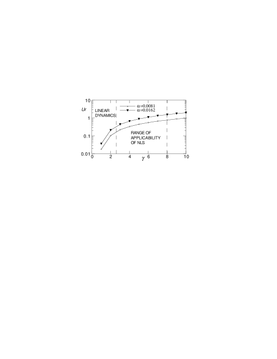
FIG. 2.: The Ursell number as a function of $\gamma$ for the JONSWAP spectrum.

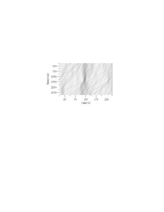
FIG. 3.: Nonlinear Schroedinger space-time evolution of a random wave field using the JONSWAP spectrum with $\gamma$=4, $\alpha$=0.0081. For details refer to the text. Gray scale ranges from 0 m (white) to 12.8 m (dark).

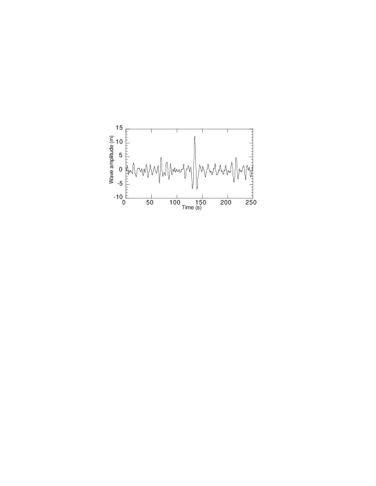
FIG. 4.: Free surface elevation $\zeta(t)$ at $x=1550$ m obtained from Fig. 3.

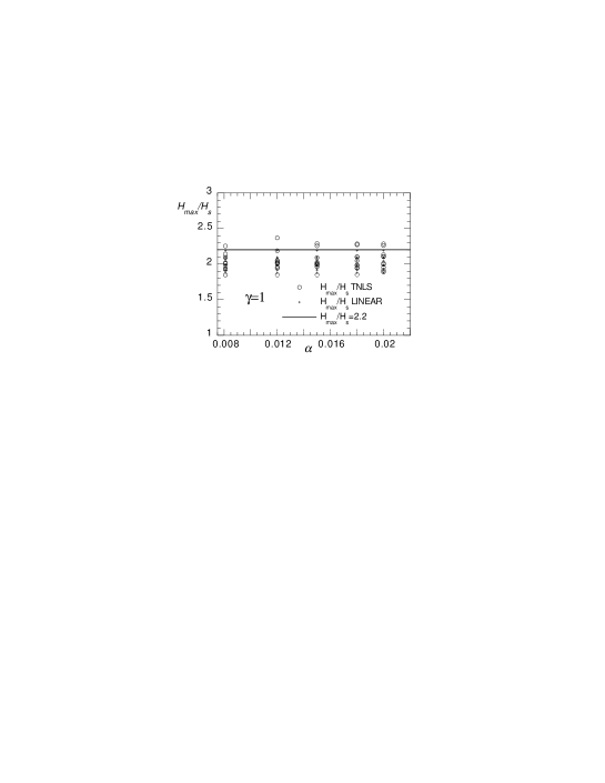
FIG. 5.: $H_{max}/H_{s}$ as a function of $\alpha$ for $\gamma=1$. Circles and crosses corresponds respectively to the nonlinear (TNLS) and linear simulations. For each value of $\alpha$, 10 different realizations corresponding to 10 different sets of random numbers have been performed.

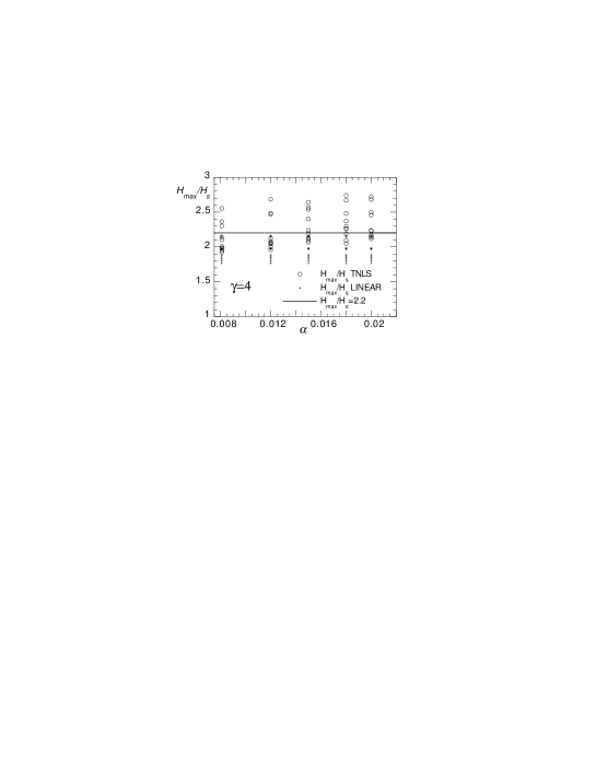
FIG. 6.: $H_{max}/H_{s}$ as a function of $\alpha$ for $\gamma=4$. Circles and crosses corresponds respectively to the nonlinear (TNLS) and linear simulations. For each value of $\alpha$, 10 different realizations corresponding to 10 different sets of random numbers have been performed.

REFERENCES

- [1] R. G. Dean, Water Wave Kinematics, 609-612, Kluwer, Amsterdam (1990).
- [2] B. S. White and B. Fornberg, J. Fluid Mech. 335, 113-138, (1998).
- [3] K. Trulsen and K. B. Dysthe, Proc. 21st Symp. on Naval Hydrodynamics, National Academy Press, 550-560, (1997).
- [4] K. B. Dysthe and K. Trulsen, Physica Sripta, T82, 48-52, (1999).
- [5] K. L. Henderson, D. H. Peregrine and J. W. Dold, Wave Motion 29 , 341-361, (1999).
- [6] M. P. Tulin and T. Waseda, J. Fluid Mech. 378, 197-232, (1999).
- [7] T. B. Benjamin and J. E. Feir, J. Fluid Mech. 27, 417-430, (1967).
- [8] H. Yuen, in Nonlinear Topics in Ocean Physics ed. A. R. Osborne, North Holland, Amsterdam, 461-498, (1991).
- [9] K. Trulsen and K. B. Dysthe, Wave Motion 24, 281-289 (1996).
- [10] K. Trulsen, I. Kliakhandler, K. Dysthe and M. Velarde, Phys. of Fluids 12, 2432-2437 (2000).
- [11] A. R. Its and V. P. Kotljarov, Dokl. Akad. Nauk. Ukrain SSR Ser. A 11, 965, (1976).
- [12] E. R. Tracy, Topics in nonlinear wave theory with applications, Ph.D. Thesis, University of Maryland (1984); E. R. Tracy and H. H. Chen, Phys. Rev. A 37, 815-839, (1988).
- [13] G. J. Komen, L. Cavaleri, M. Donelan, K. Hasselman, S. Hasselman and P. A. E. M. Janssen Dynamics and modelling of ocean waves, Cambridge University Press, (1994).
- [14] E. Lo and C. C. Mei, J. Fluid. Mech. 150, 395-416, (1985).
- [15] C. C. Mei, The Applied Dynamics of Ocean Surface Waves, Wiley and Sons, (1983).
- [16] A. R. Osborne and M. Petti, Phys. of Fluids 6, 1727-1744, (1994).
- [17] A. R. Osborne, inTopics in Ocean Physics, Proceedings of the Int. School E. Fermi, 515-550, (1982).
- [18] K. B. Dysthe, Proc. R. Soc. Lond. A 369, 105-114, (1979).
- [19] A. R. Osborne, M. Onorato and M. Serio, Phys. Lett. A 275, 386-393, (2000)
- [20] D. Resio, Private communication, Torino, October 2000.