Effect of External Noise Correlation in Optical Coherence Resonance

Abstract

Coherence resonance occurring in semiconductor lasers with optical feedback is studied via the Lang-Kobayashi model with external non-white noise in the pumping current. The temporal correlation and the amplitude of the noise have a highly relevant influence in the system, leading to an optimal coherent response for suitable values of both the noise amplitude and correlation time. This phenomenon is quantitatively characterized by means of several statistical measures.

PACS numbers: 05.40.–a, 42.65.Sf, 42.55.Px

Despite random fluctuations usually constitute a source of disorder in dynamical systems, many examples exist in which they lead instead to an increase of order in the system behavior. Among these examples, stochastic resonance stands out for its implications in many different areas of science [1]. In the conventional situation, stochastic resonance consists of an optimization due to noise of the response of a nonlinear system to a weak periodic driving [2]. But even in the absence of external periodic forcing, noise can be helpful in sustaining a coherent oscillatory response in the system, provided the operation point is close to a limit cycle [3] or within an excitable regime [4]. This phenomenon has been called coherence resonance (CR), and has been recently found also in bistable [5] and chaotic [6] systems.

One of the earliest and most influential experimental observations of stochastic resonance was made in a laser system [7]. Similarly, optical systems have also provided in recent years clear-cut examples of excitable behavior, including observations in semiconductor lasers subject to optical feedback [8, 9], lasers with saturable absorber [10], passive nonlinear ring cavities [11], lasers with injected signal [12], and self-pulsing lasers [13]. Following these studies, optical CR was predicted theoretically in the self-pulsing laser [14] and observed experimentally in the semiconductor laser with optical feedback [15]. In this latter case, noise is added to the driving current of the laser, and gives rise to a pulsed behavior in the system, in the form of sudden drop-outs in the evolution of the light intensity. The regularity of the drop-out series initially increases with increasing fluctuations, and peaks for an optimal amount of noise. The present Communication is devoted to the theoretical modeling of this situation, making use of a rate equation system including a delay term, i.e. the well-know Lang-Kobayashi (LK) model [16] generalized to take into account the insertion of external noise into the system through the laser’s pumping current.

Our results show that a white-noise assumption is not adequate to account for the observed resonant behavior. In fact, such a supposition is not realistic, due to the fast time scales in which this system evolves ($\sim$ tens of ps), smaller than or on the order of the characteristic time scales of the fastest fluctuations that can be experimentally introduced, which are restricted by 0 limitations of the electronics involved ($\sim\,$GHz). Following these considerations, we have considered a time-correlated external noise, and found that coherence is maximal not only for an optimal noise amplitude, but also for an optimal noise correlation time. In what follows, such a double coherence resonance is described in detail and characterized by suitable statistical measures.

The LK model describes the temporal evolution of the slowly varying complex envelope of the electric field $E(t)$ inside the laser and the excess carrier number $N(t)$, considering only one longitudinal mode of the solitary laser, and one single reflection from the external feedback mirror (i.e. multiple reflections are neglected, which is valid for not too large reflectivities). In dimensionless form the model reads [9, 16]:

$$\frac{dE}{dt} = \frac{1+i\alpha}{2}(G(E,N)-\gamma)\,E(t)$$ (2)

$$\qquad\qquad+\kappa e^{-i\omega\tau_{f}}E(t-\tau_{f})+\sqrt{2\beta N}\zeta(t)$$

$$\frac{dN}{dt} = \gamma_{e}\left\{C[1+\xi(t)]N_{\rm th}-N(t)\right\}-G(E,N)\,|E(t)|^{2}\,,$$ (3)

where $\gamma$ and $\gamma_{e}$ are the inverse lifetimes of photons and carriers, respectively, $C$ is the pumping rate (directly related to the driving current; $C=1$ is the solitary-laser threshold), $\alpha$ is the linewidth enhancement factor, and $\omega$ is the solitary-laser frequency. The last term in the electric-field equation represents spontaneous emission fluctuations, with $\zeta(t)$ a Gaussian white noise of zero mean and unity intensity, and $\beta$ measuring the internal noise strength. The material-gain function $G(E,N)$ is given by

$$G(E,N)=\frac{g(N(t)-N_{0})}{1+s|E(t)|^{2}}\,,$$ (4)

where $g$ is the differential gain coefficient and $s$ the saturation coefficient. The threshold carrier number is $N_{\rm th}=\gamma/g+N_{0}$. The optical feedback is described by two parameters: the feedback strength $\kappa$ and the external round–trip time $\tau_{f}$. Finally, the external noise is represented by the term $\xi(t)$, which according to the discussion made above, is taken to be a time-correlated noise of the Ornstein-Uhlenbeck type, gaussianly distributed with zero mean and correlation

$$\langle\xi(t)\xi(t^{\prime})\rangle=\frac{D}{\tau_{c}}\,e^{-(t-t^{\prime})/\tau_{c}}$$ (5)

This external noise is characterized by two parameters, its intensity $D$ and its correlation time $\tau_{c}$. The variance of the noise is given by $D/\tau_{c}$, and hence we will measure its amplitude as $\sigma=\sqrt{D/\tau_{c}}$.

The LK model with no external noise has been profusely used in the past to model the dynamics of semiconductor lasers subject to optical feedback. In particular, it satisfactorily describes the appearance of drop-outs when the system is perturbed with electrical pulses over a threshold value, with the feature that the shape of the generated (inverted) pulses is basically independent of the perturbation [9]. This behavior, which is characteristic of excitable systems and appears when the laser is operated close to the solitary laser threshold, agrees with experimental observations [8]. For larger pumping rates (but still close to the laser threshold) the intensity dropouts appear spontaneously, i.e. no external excitation is needed to produce them. Figure 1 displays an example of this behavior, in terms of the evolution of both the intensity $I(t)$ and phase difference between consecutive round-trips $\eta(t)=\phi(t)-\phi(t-\tau_{f})$, with $E(t)=\sqrt{I}\exp(i\phi)$. The occurrence of pulses in the form of power drop-outs in the intensity time series can be clearly identified, and they are seen to correspond with well-defined pulses in the electric-field phase difference.

FIG. 1.: Time evolution exhibiting drop-outs of the intensity $I$ and the corresponding pulses in the phase difference $\eta$. Parameters of the LK model are: $C=1.03$, $\gamma_{e}=6\cdot 10^{-4}$ ps^-1, $\gamma=0.158$ ps^-1, $g=2.79\cdot 10^{-9}$ ps^-1, $s=3\cdot 10^{-7}$, $\alpha=3.5$, $N_{0}=1.51\cdot 10^{8}$, $\beta=5\cdot 10^{-10}$ ps^-1, $\kappa=0.025$ ps^-1, $\tau_{f}=2.4$ ns, $\omega\tau_{f}=2$, and $D=0$.

It should be noted that the intensity time trace shown in Fig. 1(a) has been filtered to $100$ MHz, in order to mimic the bandwidth effect of typical photodetectors. For large enough filtering bandwidth (or for no filtering at all), the corresponding evolution takes the form of ultrashort intensity pulses (with durations on the order of tens of ps) [17], whose envelope exhibits the low-frequency drop-outs shown in Fig. 1(a).

Since the internal spontaneous-emission noise $\zeta(t)$ cannot be experimentally controlled, we now turn our attention to the effect of the external noise $\eta(t)$ upon the system. This effect can be understood by examining the mechanism behind the above-mentioned power drop-outs, which is well understood in the framework of the LK model (i.e. under the assumption of single-mode operation of the laser). This model exhibits multiple coexisting fixed points, which appear in pairs of solutions called modes and antimodes. The antimodes are saddle points, and most of the modes are also unstable due to a Hopf bifurcation [18]. However, at least one of the modes (the one with maximum power) is stable. In this complex phase-space landscape, a large enough fluctuation may be able to take the system away from the basin of attraction of the stable fixed point and, upon collision with a neighboring antimode, produce a sudden increase in the phase difference [see Fig. 1(b)] which corresponds to a power drop-out. The corresponding escape time, also called activation time $t_{a}$, is a random variable whose average decreases with the intensity of the external noise according to Kramers’ law [19]. Following the drop-out, a build-up process begins in which the system undergoes a chaotic itinerancy around the Hopf-unstable modes, jumping consecutively from one to the next while being drifted back towards the stable maximum-gain mode [20]. For small intensities of the external noise, the excursion time $t_{e}$ required by this process is basically independent of noise, and has the role of a refractory time during which no drop-outs can be induced. As noise intensity increases the escape events become more frequent, reducing the standard deviation of the interspike intervals accordingly. A minimum of variability occurs for an optimal amount of noise when the drop-out separation is of the order of $t_{e}$. Beyond that point, noise intensity is large enough to produce escapes before the build-up process is finished (i.e. before the stable mode is reached), which leads to an irregular series of pulses. This sequence of events is depicted in Fig. 2, which shows three time traces of the phase difference $\eta(t)$ for increasing amplitudes of the external noise, keeping its correlation time constant. In this case, the semiconductor laser is biased at $1\%$ above the solitary-laser threshold, a situation for which the system is stable in the absence of external noise. A small amount of noise produces infrequent drop-outs [Fig. 2(a)], which become more numerous and regular as the noise amplitude increases [Fig. 2(b)]. For large noise strengths the pulses become increasingly irregular, both in separation and in amplitude [Fig. 2(c)]. Hence, an optimal amplitude of the external noise exists for which the coherence of the pulsed output of the laser is optimal.

In order to quantitatively characterize this effect, we compute the standard deviations $R_{\theta}$ and $R_{\mu}$ of the normalized drop-out separation $\theta=T/\langle T\rangle$ and normalized drop-out amplitude $\mu=A/\langle A\rangle$, respectively [15], where the statistical averages are performed over both time and different realizations of the noise. Numerically, to detect a drop-out we study the behavior of the phase difference $\eta(t)$, since its variation is smoother than that of the intensity, and easier to characterize. A drop-out occurrence is recorded when the phase difference $\eta$ suddenly increases in a fixed large amount (e.g. $12\pi$ in our case) [9]. The drop-out amplitude $A$ is a measure of the total height of the phase pulse.

FIG. 2.: Temporal behavior of the phase difference $\eta$ for increasing noise amplitude: (a) $\sigma=7.36\cdot 10^{-2}$, (b) $\sigma=9.35\cdot 10^{-2}$, and (c) $\sigma=1.60\cdot 10^{-1}$. In all cases we have kept the correlation time constant, $\tau_{c}=24$ ps. Other parameters are those of Fig. 1, except $C=1.01$.

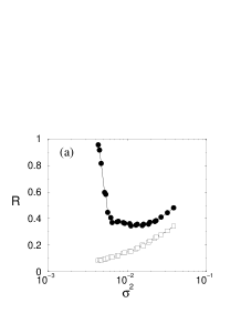
FIG. 3.: Statistical characterization of the noise-amplitude coherence resonance. (a) Standard deviations $R_{\theta}$ (full circles) and $R_{\mu}$ (empty squares), and (b) joint entropy $H(\theta,\mu)$ as a function of the external noise amplitude. The time correlation of the noise is fixed to $\tau_{c}=24$ ps. Other parameters are those of Fig. 2.

We have computed the standard deviations $R_{\theta}$ and $R_{\mu}$ for increasing noise amplitude, averaging up to 20,000 drop-outs in each measure. The result is plotted in Fig. 3(a), and confirms the qualitative conclusions that have been drawn above from Fig. 2, at least as far as the variability of the pulse separation, $R_{\theta}$, is concerned. This quantity is a non-monotonic function of the noise amplitude, being minimal for an optimal amount of noise. The irregularity of the drop-out amplitudes, on the other hand, increases monotonically with noise. This result coincides with experimental observations [15], and reflects the fact that the frequency with which noise breaks up the build-up process increases steadily with the amount of noise added.

In order to take into account both the drop-out separation and amplitude simultaneously in the determination of the signal’s regularity, it is useful to define a joint entropy $H(\theta,\mu)$ of the two quantities, where $H=-\sum P\log P$, with $P$ the joint probability density of the two random variables [21]. For the case of two Gaussian independent random variables the following relation holds [15]: $\exp(H(\theta,\mu))=2\pi eR_{\theta}R_{\mu}$. We will assume that this result is approximately valid in our case, and compute the joint entropy accordingly. The result is given in Fig. 3(b), which shows again a maximum regularity of the drop-out series for an optimal noise amplitude, this time taking into account both the pulse separation and amplitude. In fact, the minimum is in this case more clearly defined.

We note that all results presented so far have been computed for a fixed correlation time of the noise $\tau_{c}=24$ ps, on the order of the fast time scale of the deterministic dynamics. In fact, as the white-noise limit is approached the amount of noise necessary to obtain similar effects climbs up to unreasonably high values. The reason is that the carrier dynamics acts as a frequency filter for the external noise [see equation for $N(t)$ in (2)], which also prevents the system from responding to high-frequency modulations of the pump current. Therefore, most of the power of a white noise has no effect upon the system dynamics, and the noise intensity needs to be very large in order to have a noticeable influence (a similar effect has been observed in periodic-modulation studies [22]). In the opposite frequency limit a similar situation occurs: for low-frequency forcing the carrier dynamics has enough time to follow the modulation, and the system responds simply with a modulated output. Only for intermediate frequencies will the external forcing be able to influence the drop-out statistics and enhance the coherent response of the system. In order to verify this conjecture, we now fix the amplitude $\sigma=\sqrt{D/\tau_{c}}$ of the external noise and analyze the behavior of the system for an increasing correlation time of the Ornstein-Uhlenbeck noise defined by Eq. (5). The result is shown in Fig. 4 for three different values of $\tau_{c}$. It can be seen that the regularity of the pulsed time series is maximal for intermediate values of the noise correlation time.

We quantify again the qualitative observation made in the previous paragraph by computing the standard deviations $R_{\theta}$ and $R_{\mu}$, and the joint entropy $H(\theta,\mu)$ of the normalized drop-out separation and amplitude. The results, shown in Fig. (5), exhibit the same behavior as in the case of an increasing noise amplitude. Coherence of the pulsed behavior is in this case maximal for a correlation time of the noise $\tau_{c}\sim 30$ ps. This behavior can be interpreted as a resonance with the fast deterministic dynamics of the system. A similar resonance has been recently observed experimentally in a chemical excitable medium [23].

FIG. 4.: Temporal behavior of the phase difference $\eta$ for increasing noise correlation time: (a) $\tau_{c}=15.8$ ps, (b) $\tau_{c}=57.6$ ps, and (c) $\tau_{c}=153.2$ ps. In all cases we have kept the noise amplitude constant, $\sigma=0.079$. Other parameters are those of Fig. 2.

  

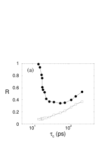
FIG. 5.: Statistical characterization of the noise-correlation coherence resonance. (a) Standard deviations $R_{\theta}$ (full circles) and $R_{\mu}$ (empty squares), and (b) joint entropy $H(\theta,\mu)$ as a function of the noise correlation time. The noise amplitude is fixed to $\sigma=0.079$. Other parameters are those of Fig. 4.

In conclusion, we have shown the existence of double coherence resonance in an excitable optical system (a semiconductor laser with optical feedback) driven by an external correlated noise. The assumption of a non-delta temporal correlation of the noise is fully meaningful, given the fast characteristic time scale of the deterministic dynamics of the system. The pulsed response of the laser, which takes the form of intensity drop-outs, exhibits a maximal coherence for optimal values of both the amplitude and correlation time of the external noise. These results agree satisfactorily with previous experimental observations. Other recent investigations have analyzed the influence of correlated noise in model systems exhibiting coherence resonance [24], but in those cases the corresponding deterministic system lacked a natural second time scale (different from the optimal pulse separation) which could account for the resonance with respect to the noise correlation time. In the present case, however, such a time scale does exist naturally in the system.

We acknowledge financial support from MCyT (Spain), under projects BFM2000-1108 and BFM2000-0624, and from DGES (Spain), under projects PB98-0935 and PB97-0141.

REFERENCES

- [1] K. Wiesenfeld and F. Moss, Nature 373, 33 (1995).
- [2] L. Gammaitoni, P. Hänggi, P. Jung, and F. Marchesoni, Rev. Mod. Phys. 70, 223 (1998).
- [3] H. Gang, T. Ditzinger, C.Z. Ning, and H. Haken, Phys. Rev. Lett. 71, 807 (1993); W.J. Rappel and S.H. Strogatz, Phys. Rev. E 50, 3249 (1994).
- [4] A. Pikovsky and J. Kurths, Phys. Rev. Lett. 78, 775 (1997).
- [5] B. Lindner and L. Schimansky-Geier, Phys. Rev. E 61, 6103 (2000).
- [6] C. Palenzuela, R. Toral, C.R. Mirasso, O. Calvo, and J.D. Gunton, preprint cond-mat/0007371.
- [7] B. McNamara, K. Wiesenfeld, and R. Roy, Phys. Rev. Lett. 60, 2626 (1988).
- [8] M. Giudici, C. Green, G. Giacommelli, U. Nespolo, and J.R. Tredicce, Phys. Rev. E 55, 6414 (1997).
- [9] J. Mulet and C.R. Mirasso, Phys. Rev. E 59, 5400 (1999).
- [10] F. Plaza, M.G. Velarde, F.T. Arecchi, S. Boccaletti, and M. Ciofini, Europhys. Lett. 38, 85 (1997).
- [11] W. Lu, D. Yu, and R.G. Harrison, Phys. Rev. A 58, R809 (1998).
- [12] P. Coullet, O. Daboussy, and J.R. Tredicce, Phys. Rev. E 58, 5347 (1998).
- [13] J.L.A. Dubbeldam, and B. Krauskopf, Opt. Commun. 159, 325 (1999).
- [14] J.L.A. Dubbeldam, B. Krauskopf, and D. Lenstra, Phys. Rev. E 60, 6580 (1999).
- [15] G. Giacomelli, M. Giudici, S. Balle, and J.R. Tredicce, Phys. Rev. Lett. 84, 3298 (2000).
- [16] R. Lang and K. Kobayashi, IEEE J. Quantum Electron. 16, 347 (1980).
- [17] I. Fischer, G.H.M. van Tartwijk, A.M. Levine, W. Elsäßer, E. Göbel, and D. Lenstra, Phys. Rev. Lett. 76, 220 (1996); D.W. Sukow, T. Heil, I. Fischer, A. Gavrielides, A. Hohl-AbiChedid, and W. Elsäßer, Phys. Rev. A 60, 667 (1999).
- [18] A.M. Levine, G.H.M. van Tartwijk, D. Lenstra, and T. Erneux, Phys. Rev. A 52, R3436 (1995).
- [19] P. Hänggi, P. Talkner, and M. Borkovec, Rev. Mod. Phys. 62, 251 (1990).
- [20] T. Sano, Phys. Rev. A 50, 2719 (1994).
- [21] R. Badii and P. Politi, Complexity: hierarchical structures and scaling in physics (Cambridge University Press, Cambridge, 1997).
- [22] D.W. Sukow and D.J. Gauthier, IEEE J. Quantum Electron. 36, 175 (2000).
- [23] I. Sendiña-Nadal, S. Alonso, V. Pérez-Muñuzuri, M. Gómez-Gesteira, V. Pérez-Villar, L. Ramírez-Piscina, J. Casademunt, J. M. Sancho, and F. Sagués, Phys. Rev. Lett. 84, 2734 (2000).
- [24] J.M. Casado, Phys. Lett. A 235, 489 (1997); S. Zhong and H.W. Xin, Chem. Phys. Lett. 333, 133 (2001).