Wavy stripes and squares in zero Prandtl number convection

Abstract

A simple model to explain numerically observed behaviour of chaotically varying stripes and square patterns in zero Prandtl number convection in Boussinesq fluid is presented. The nonlinear interaction of mutually perpendicular sets of wavy rolls, via higher order modes, may lead to a competition between the two sets of rolls. The appearance of square patterns is due to secondary forward Hopf bifurcation of a set of wavy rolls.

The study of low Prandtl number thermal convection [1-13] has been long motivated by its importance in geophysical and astrophysical problems. The hydrodynamical equations of thermal convection in Boussinesq fluids involve two types of nonlinearity. The first describes self-interaction ${\bf v.\nabla v}$ of the velocity field ${\bf v}$, and the second nonlinearity ${\bf v.\nabla}\theta$ results from the advection of the temperature fluctuation $\theta$ by the velocity field. The nonlinearity ${\bf v.\nabla}\theta$ may be neglected in the asymptotic limit of zero Prandtl number spiegel . The linearly growing two-dimensional (2D) rolls then become exact solutions of nonlinear equations, if stress-free boundary conditions are considered. This makes this limit interesting even from purely theoretical point. Thual thual recently showed by a most general 3D direct numerical simulations (DNS) of zero $P$ asymptotic equations that the solutions do not blow up. The comparison with full Boussinesq equations with both nonlinearities also reproduced zero P results. This DNS showed many interesting patterns including the possibility of square patterns in zero $P$ Boussinesq fluids with stress-free boundaries for $1.05<r(=R/R_{c})<1.7$, where the critical Rayleigh number $R_{c}=27\pi^{4}/4$. However, the mechanism of generation of square patterns in zero $P$ convection remains unexplained. A nonlinear interaction between 2D rolls cannot generate either square or hexagonal patterns kumar for zero $P$ asymptotic equations as growing straight 2D rolls are their exact solutions. The streamlines in DNS thual support this view. On the other hand, the mechanism of prevention of continuous growth of 2D rolls approximately $0.5\%$ above the onset of convection was captured in a simple dynamical system kft , which agreed well with the results of DNS in its validity range. This model suggested that 2D rolls undergo self-tuned nonlocal wavy instability kft , which prevents their further growth. The nonlinear superposition of two sets of wavy rolls may result in the form of square patterns. However, this proposition is not analyzed so far.

We present in this article a simple dynamical system, which describes nonlinear interaction between mutually perpendicular sets of wavy rolls, and captures the mechanism of selection of square patterns in zero Prandtl number Boussinesq fluid. We show that the generation of vertical vorticity is important in addition to higher order modes to provide nonlinear coupling among mutually perpendicular sets of rolls. This is qualitatively different from the case of high Prandtl number convection das where nonlinear interaction of two sets of straight rolls may give rise to square patterns even in absence of vertical vorticity. The mutually perpendicular sets of wavy rolls interact through distortions in the vertical velocity as well as the vertical vorticity. The nonlinear interaction give rise to complex convective patterns. The sequence of wavy stripe along $x-$axis, square patterns, and $y-$ axis is chaotic. The generation of square patterns from wavy rolls is via forward Hopf bifurcation.

We consider a thin horizontal layer of fluid of thickness $d$, confined between two conducting boundaries, and heated underneath. The fluid motion is assumed to be governed by zero Prandtl number Boussinesq equations spiegel ; thual , which may be put in the following dimensionless form:

$$\partial_{t}{\nabla^{2}v_{3}} = {\nabla}^{4}v_{3}+R{{\nabla}_{H}}^{2}\theta$$ (1)

$$- {\bf{e_{3}}}.{\bf{\nabla}}\times[({\bf{\omega}}.{\bf{\nabla}}){\bf v}-({\bf v}.{\bf{\nabla}}){\bf{\omega}}]$$

$$\partial_{t}{\omega_{3}} = {\nabla}^{2}{\omega_{3}}+[({\bf{\omega}}.{\bf{\nabla}}){v_{3}}-({\bf v}.{\bf{\nabla}}){\omega_{3}}]$$ (2)

$${\nabla}^{2}\theta = -{v_{3}}$$ (3)

where ${\bf v}\equiv(v_{1},v_{2},v_{3})$ is the velocity field, $\theta$ the deviation from the conductive temperature profile, and $\omega={\nabla}\times{\bf v}\equiv(\omega_{1},\omega_{2},\omega_{3})$ the vorticity field. The Rayleigh number R is defined as $R=\frac{\alpha(\Delta T)g{d}^{3}}{\nu\kappa}$, where $\alpha$ is the coefficient of thermal expansion of the fluid, g the acceleration due to gravity. The unit vector ${\bf e_{3}}$ is directed vertically upward, which is assumed to be the positive direction of $x_{3}$-axis. The boundary conditions at the stress-free conducting flat surfaces imply $\theta=v_{3}=\partial_{33}{v_{3}}=0$ at $x_{3}=0,1$. and ${{\nabla}_{H}}^{2}=\partial_{11}+\partial_{22}$ is the horizontal Laplacian.

We employ the standard Galerkin procedure to describe the convection patterns in the form two sets mutually perpendicular sets of wavy rolls, and the patterns resulting due to their nonlinear superposition. The spatial dependence of the vertical velocity and the vertical vorticity are expanded in Fourier series, which is compatible with the stress-free flat conducting boundaries and periodic boundary conditions in the horizontal plane. As DNS shows either standing waves or stationary patterns, all time-dependent Fourier amplitudes are set to be real. The expansion for all the fields are truncated to describe convective structures in the form of straight cylindrical (2D) rolls, wavy (3D) rolls, and patterns arising due to their nonlinear superposition. The vertical velocity $v_{3}$ and the vertical vorticity $\omega_{3}$ then read as

$$v_{3} = [W_{101}(t)\cos{(kx_{1})}+W_{011}(t)\cos{(kx_{2})}]\sin{(\pi x_{3})}$$ (4)

$$+ W_{211}(t)\cos{(2kx_{1})}\cos{(kx_{2})}\sin{(\pi x_{3})}$$

$$+ W_{121}(t)\cos{(kx_{1})}\cos{(2kx_{2})}\sin{(\pi x_{3})}$$

$$+ W_{111}(t)\sin{(kx_{1})}\sin{(kx_{2})}\sin{(\pi x_{3})}$$

$$+ W_{112}(t)\cos{(kx_{1})}\cos{(kx_{2})}\sin{(2\pi x_{3})}+....$$

$$\omega_{3} = Z_{010}(t)\cos{(kx_{2})}+Z_{100}(t)\cos{(kx_{1})}$$ (5)

$$+ Z_{111}(t)\cos{(kx_{1})}\cos{(kx_{2})}\cos{(\pi x_{3})}$$

$$+ [Z_{201}(t)\cos{(2kx_{1})}+Z_{021}(t)\cos{(2kx_{2})}]\cos{(\pi x_{3})}$$

$$+ [Z_{102}(t)\cos{(kx_{1})}+Z_{012}(t)\cos{(kx_{2})}]\cos{(2\pi x_{3})}$$

$$+ Z_{210}(t)\cos{(2kx_{1})}\cos{(kx_{2})}$$

$$+ Z_{120}(t)\cos{(kx_{1})}\cos{(2kx_{2})}+....$$

The temperature field is slaved in the limit of zero Prandtl number, and it can be computed from Eq. 3. The horizontal components $v_{1},v_{2}$ of the velocity field and the same ($\omega_{1},\omega_{2}$) of the vorticity field are then computed by their solenoidal character. We now project the hydrodynamical equations $1-3$ into these modes to get the following dynamical system

$$\dot{\vec{X}} = \frac{3\pi^{2}}{2}(r-1){\vec{X}}+\frac{1}{6}\left(\begin{array}[]{c}{S\zeta_{1}}\\ -{S\zeta_{2}}\end{array}\right)+\frac{1}{4}\left(\begin{array}[]{c}{S\phi_{1}}\\ -{S\phi_{2}}\end{array}\right)+\frac{1}{20}\left(\begin{array}[]{c}{S\psi_{1}}\\ -{S\psi_{2}}\end{array}\right)$$ (12)

$$- \frac{1}{3\pi}{\eta}{\vec{\zeta}}-\frac{1}{6\pi}{\eta}{\vec{\phi}}-\frac{1}{30\pi}{\eta}{\vec{\psi}}-\frac{2}{15\pi}\left(\begin{array}[]{c}{\chi_{2}}{\psi_{2}}\\ {\chi_{1}}{\psi_{1}}\end{array}\right)-\frac{\pi}{24}T{\vec{Y}}+\frac{\pi}{4}\left(\begin{array}[]{c}{TX_{2}}\\ {TX_{1}}\end{array}\right)$$ (17)

$$\dot{S} = \frac{\pi^{2}}{16}(27r-32)S-{\zeta_{1}}{X_{1}}+{\zeta_{2}}{X_{2}}+\frac{1}{10}(-{X_{1}}{\psi_{1}}+{X_{2}}{\psi_{2}})+\frac{1}{2}(-{X_{1}}{\phi_{1}}+{X_{2}}{\phi_{2}})$$ (18)

$$+ \frac{3}{100}({\psi_{1}}{Y_{2}}-{\psi_{2}}{Y_{1}})+\frac{3}{20}({\phi_{1}}{Y_{2}}-{\phi_{2}}{Y_{1}})+\frac{3}{10}({\zeta_{1}}{Y_{2}}-{\zeta_{2}}{Y_{1}})$$

$$\dot{T} = \frac{\pi^{2}}{100}(27r-500)T-\frac{3\pi}{5}{X_{1}}{X_{2}}-\frac{13\pi}{50}\vec{X}.\vec{Y}+\frac{3}{40}S({\chi_{1}}-{\chi_{2}})-\frac{63\pi}{500}{Y_{1}}{Y_{2}}$$ (19)

$$- \frac{1}{10\pi}\eta({\chi_{1}}+{\chi_{2}})-\frac{2}{25\pi}({\psi_{1}}{\phi_{2}}+{\psi_{2}}{\phi_{1}})-\frac{4}{5\pi}({\zeta_{2}}{\phi_{1}}+{\zeta_{1}}{\phi_{2}})$$

$$\dot{\vec{Y}} = \frac{\pi^{2}}{98}(135r-343)\vec{Y}+\frac{31\pi}{28}T\vec{X}+\frac{3}{28}\left(\begin{array}[]{c}{S\phi_{2}}\\ -{S\phi_{1}}\end{array}\right)+\frac{9\pi}{40}\left(\begin{array}[]{c}T{Y_{2}}\\ T{Y_{1}}\end{array}\right)$$ (24)

$$- \frac{1}{14\pi}\left(\begin{array}[]{c}{\eta}{\phi_{2}}\\ {\eta}{\phi_{1}}\end{array}\right)+\frac{3}{28}\left(\begin{array}[]{c}{S\psi_{2}}\\ -{S\psi_{1}}\end{array}\right)-\frac{9}{70\pi}\left(\begin{array}[]{c}{\eta}{\psi_{2}}\\ {\eta}{\psi_{1}}\end{array}\right)-\frac{8}{35\pi}\left(\begin{array}[]{c}{\chi_{2}}{\psi_{1}}\\ {\chi_{1}}{\psi_{2}}\end{array}\right)$$ (33)

$$+ \frac{9}{14}\left(\begin{array}[]{c}{S\zeta_{2}}\\ -{S\zeta_{1}}\end{array}\right)-\frac{1}{7\pi}\left(\begin{array}[]{c}{\eta}{\zeta_{2}}\\ {\eta}{\zeta_{1}}\end{array}\right)-\frac{2}{7\pi}\left(\begin{array}[]{c}{\chi_{1}}{\phi_{1}}\\ {\chi_{2}}{\phi_{2}}\end{array}\right)-\frac{4}{7\pi}\left(\begin{array}[]{c}{\zeta_{1}}{\chi_{1}}\\ {\zeta_{2}}{\chi_{2}}\end{array}\right)$$ (42)

$$\dot{\vec{\zeta}} = -\frac{\pi^{2}}{2}\vec{\zeta}+\frac{\pi^{2}}{8}\left(\begin{array}[]{c}SX_{1}\\ -SX_{2}\end{array}\right)+\frac{3\pi^{2}}{80}\left(\begin{array}[]{c}SY_{2}\\ -SY_{1}\end{array}\right)+\frac{\pi}{8}{\eta}{\vec{X}}-\frac{\pi}{8}\left(\begin{array}[]{c}{\chi_{2}}{X_{2}}\\ {\chi_{1}}{X_{1}}\end{array}\right)$$ (49)

$$- \frac{\pi}{80}\left(\begin{array}[]{c}{\eta}{Y_{2}}\\ {\eta}{Y_{1}}\end{array}\right)+\frac{\pi}{4}\left(\begin{array}[]{c}T{\phi_{2}}\\ T{\phi_{1}}\end{array}\right)+\frac{\pi}{20}\left(\begin{array}[]{c}{\chi}_{1}Y_{1}\\ {\chi}_{2}X_{2}\end{array}\right)$$ (56)

$$\dot{\eta} = -2{\pi^{2}}{\eta}+\pi{\vec{\zeta}}.{\vec{X}}+\frac{3\pi}{2}\vec{\phi}.\vec{X}-\frac{\pi}{2}{\vec{\psi}}.{\vec{X}}+\frac{\pi}{8}T({\chi_{1}}+{\chi_{2}})-\frac{7\pi}{20}({\phi_{2}}{Y_{1}}+{\phi_{1}}{Y_{2}})$$ (57)

$$+ \frac{3\pi}{10}({\zeta_{2}}{Y_{1}}+{\zeta_{1}}{Y_{2}})+\frac{\pi}{20}({\psi_{1}}{Y_{2}}+{\psi_{2}}{Y_{1}})$$

$$\dot{\vec{\psi}} = -\frac{5\pi^{2}}{2}{\vec{\psi}}+\frac{\pi^{2}}{8}\left(\begin{array}[]{c}-SX_{1}\\ SX_{2}\end{array}\right)+\frac{7\pi}{8}{\eta}{\vec{X}}+{\pi}\left(\begin{array}[]{c}{\chi_{1}}X_{2}\\ {\chi_{2}}X_{1}\end{array}\right)+\frac{9\pi_{2}}{80}\left(\begin{array}[]{c}S{Y_{2}}\\ {-SY_{1}}\end{array}\right)$$ (64)

$$+ \frac{5\pi}{4}\left(\begin{array}[]{c}T{\phi_{2}}\\ T{\phi_{1}}\end{array}\right)+\frac{13\pi}{80}\left(\begin{array}[]{c}{\eta}{Y_{2}}\\ {\eta}{Y_{1}}\end{array}\right)+\frac{11\pi}{40}\left(\begin{array}[]{c}{\chi_{2}}{Y_{1}}\\ {\chi_{1}}{Y_{2}}\end{array}\right)$$ (71)

$$\dot{\vec{\phi}} = -\frac{9\pi^{2}}{2}{\vec{\phi}}+\frac{\pi^{2}}{8}\left(\begin{array}[]{c}{-SX_{1}}\\ {SX_{2}}\end{array}\right)-\frac{3\pi}{8}\left(\begin{array}[]{c}{\chi_{2}}{X_{2}}\\ {\chi_{1}}{X_{1}}\end{array}\right)-\frac{\pi}{8}\eta{\vec{X}}+\frac{\pi}{2}\left(\begin{array}[]{c}{T\zeta_{2}}\\ {T\zeta_{1}}\end{array}\right)$$ (78)

$$- \frac{\pi}{4}\left(\begin{array}[]{c}T{\psi_{2}}\\ T{\psi_{1}}\end{array}\right)+\frac{3\pi_{2}}{80}\left(\begin{array}[]{c}{-SY_{2}}\\ {SY_{1}}\end{array}\right)+\frac{9\pi}{80}\left(\begin{array}[]{c}\eta{Y_{2}}\\ \eta{Y_{1}}\end{array}\right)+\frac{\pi}{20}\left(\begin{array}[]{c}{\chi_{1}}{Y_{1}}\\ {\chi_{2}}{Y_{2}}\end{array}\right)$$ (87)

$$\dot{\vec{\chi}} = -3{\pi^{2}}{\vec{\chi}}+\frac{3\pi}{2}\left(\begin{array}[]{c}{\phi_{2}}{X_{1}}\\ {\phi_{1}}{X_{2}}\end{array}\right)+\frac{3\pi^{2}}{8}\left(\begin{array}[]{c}{-ST}\\ {ST}\end{array}\right)+\frac{3\pi}{8}\left(\begin{array}[]{c}{\eta T}\\ {\eta T}\end{array}\right)$$ (94)

$$+ \pi\left(\begin{array}[]{c}{\zeta_{2}}{X_{1}}\\ {\zeta_{1}}{X_{2}}\end{array}\right)+\frac{\pi}{5}\left(\begin{array}[]{c}{\phi_{1}}{Y_{1}}\\ {\phi_{2}}{Y_{2}}\end{array}\right)+\frac{2\pi}{5}\left(\begin{array}[]{c}{\zeta_{1}}{Y_{1}}\\ {\zeta_{2}}{Y_{2}}\end{array}\right)+\frac{\pi}{10}\left(\begin{array}[]{c}{\psi_{2}}{Y_{2}}\\ {\psi_{1}}{Y_{1}}\end{array}\right)$$ (103)

where ${\vec{X}}$ $\equiv$ $\left(\begin{array}[]{c}X_{1}\\ X_{2}\end{array}\right)$ $=$ $\left(\begin{array}[]{c}{W_{101}}\\ {W_{011}}\end{array}\right)$, ${\vec{Y}}$ $\equiv$ $\left(\begin{array}[]{c}Y_{1}\\ Y_{2}\end{array}\right)$ $=$ $\left(\begin{array}[]{c}{W_{211}}\\ {W_{121}}\end{array}\right)$, $S=W_{111}$, $T=W_{112}$ , ${\vec{\zeta}}$ $\equiv$ $\left(\begin{array}[]{c}{\zeta_{1}}\\ {\zeta_{2}}\end{array}\right)$ $=$ $\left(\begin{array}[]{c}{Z_{010}}\\ {Z_{100}}\end{array}\right)$, ${\vec{\phi}}\equiv\left(\begin{array}[]{c}{\phi_{1}}\\ {\phi_{2}}\end{array}\right)$ $=$ $\left(\begin{array}[]{c}{Z_{012}}\\ {Z_{102}}\end{array}\right)$, ${\vec{\psi}}$ $\equiv$ $\left(\begin{array}[]{c}{\psi_{1}}\\ {\psi_{2}}\end{array}\right)$ $=$ $\left(\begin{array}[]{c}{Z_{210}}\\ {Z_{120}}\end{array}\right)$, ${\vec{\chi}}$ $\equiv$ $\left(\begin{array}[]{c}{\chi_{1}}\\ {\chi_{2}}\end{array}\right)$ $=$ $\left(\begin{array}[]{c}{Z_{201}}\\ {Z_{021}}\end{array}\right),$ and ${\eta}={Z_{111}}$. All roman characters stand for velocity modes, and greek letters stand for vorticity modes.

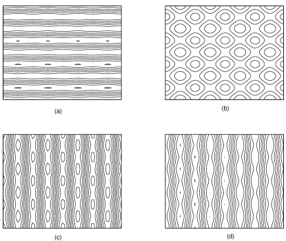
Figure 1: Four different patterns varying chaotically in time for $r=1.11$: (a) wavy rolls along x-axis, (b) square pattern, (c) patchwork quilt pattern , and (d) wavy rolls along y-axis.

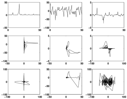
Figure 2: The top row (starting from left) shows chaotic evolution of $W_{101}$, $W_{011}$, and $W_{112}$ for $r=1.11$. The second row shows projections of phase space plot in $W_{011}-W_{101}$, $W_{112}-W_{101}$, and $W_{112}-W_{011}$ planes respectively. The third row contains projections of phase space plot in $Z_{100}-Z_{010}$, $Z_{010}-W_{101}$, and $W_{011}-Z_{100}$ planes respectively.

There is no fixed points in this model as growing straight rolls are exact solutions of the problem. We now numerically integrate this dynamical system to investigate time dependent solutions. For each value of $r$, we start integration with randomly chosen initial conditions. We integrate for long periods ($\approx 100-200$ times the viscous diffusive time scale) to ignore the transient effects. We increase $r$ in small steps $\Delta r$ ($=0.01$) and repeat the above mentioned procedure. We get chaotic solutions for $1.11\leq r\leq 1.42$ for $k_{x}=k_{y}=k_{c}=\pi/\sqrt{2}$, which is in qualitative agreement with the DNS of Thual thual . For $r<1.11$ we observe wavy rolls oscillating chaotically, and for $r\geq 1.11$ we observe chaotic sequence of wavy rolls, squares, and asymmetric squares. For $r>1.42$ and $k_{x}=k_{y}=k_{c}$, the model is not good enough as the anharmonicity in various fields is very high in the limit of zero Prandtl number. This is natural as there is no additional heat flux across the fluid layer due to convective motion. The extra energy is consumed by the internal dynamics.

Figure 1 shows competition of various patterns for $r=1.11$. Two mutually perpendicular sets of wavy rolls compete with each other. This leads to square as well as patchwork quilt patterns. The sequence of occurrence of these patterns is not periodic but chaotic. Notice that the square pattern (see Fig. 1) consists of two sets of squares. A small (big) square has four big (small) squares as its nearest neighbors (Fig. 1 b). This feature of the square pattern is qualitatively new for convection in Boussinesq fluid.

The top row of Fig. 2 (starting from left) shows time evolution of velocity modes $W_{101}$, $W_{011}$ and $W_{112}$ respectively after integration of the model for a period more than $200\times$ viscous time scale. The signal is chaotic. The second and third rows of Fig. 2 show various projections of the phase plots in fifteen dimensional phase space. Figure 3 shows time variation of the spatially average energy $E_{av}=\frac{1}{2}<v_{1}^{2}+v_{2}^{2}+v_{3}^{2}>_{x_{1}x_{2}x_{3}}.$ The averaged energy shows relaxation oscillation in irregular way. This is also a common feature of DNS thual .

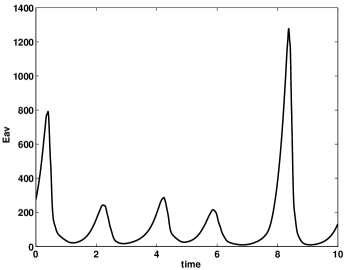
Figure 3: Time variation of spatially averaged energy in a unit cell.

We have presented in this paper a simple model which explains the mechanism responsible for generation of square patterns in zero Prandtl number limit in Boussinesq fluids. As the Rayleigh number is increased, one set of wavy rolls oscillating chaotically become unstable. Another set of wavy rolls are generated in a direction perpendicular to the former one. The nonlinear superposition of these wavy rolls give rise to squares and other complex patterns. The vertical vorticity modes with nonzero mean in vertical direction are responsible for the wavy nature of rolls at very close to the instability onset in case of stress-free bounding surfaces. These modes stop the unlimited growth of the $2D$ rolls. The DNS thual also showed wavy rolls rather than straight rolls. The nonlinear modes depending on both the horizontal coordinates facilitate the exchange of energy between two sets of wavy rolls.

Acknowledgements: Pinaki Pal acknowledges support from CSIR, India through its grants.

References

• (1) E. A. Spiegel, J. Geophys. Research 67, 3063 (1962).
• (2) R. H. Karaichnan and E. A. Spiegel, Phys. Fluids 5, 583 (1962).
• (3) J. R. Herring, Woods Hole Oceanogr. Inst. Tech. Rep., WHOI-70-01 (1970).
• (4) M. R. Proctor, J. Fluid Mech. 82, 97 (1977).
• (5) R. M. Clever and F. H. Busse, J. Fluid Mech. 102, 63 (1981).
• (6) F. H. Busse and R. M. Clever, J. Fluid Mech. 102, 75 (1981).
• (7) P. Sulem, C. Sulem, and O. Thual, Prog. Astro. Aeronaut. 100, 125 (1985).
• (8) A. Chiffaudel, S. Fauve, and B. Perrin, Europhys. Lett. 4, 555 (1987).
• (9) M. Meneguizzi, C. Sulem, P. L. Sulem, and O. Thual, J. Fluid Mech. 182, 169 (1987).
• (10) V. Croquette, Contem. Phys. 30, 113 (1989); 30 153 (1989).
• (11) K. Kumar, Woods Hole Oceanogr. Inst. Tech. Rep., WHOI-90-01 (1990).
• (12) O. Thual, J. Fluid Mech. 240, 229 (1992).
• (13) K. Kumar, S. Fauve, and O. Thual, J. Phys. II France 6, 945 (1996).
• (14) A. Das, U. Ghosal, and K. Kumar, Phys. Rev. E (2000).