Dissipation induced Instabilities and the Mechanical Laser

Abstract

We study the 1:1 resonance for perturbed Hamiltonian systems with small dissipative and energy injection terms. These perturbations of the 1:1 resonance exhibit dissipation induced instabilities. This mechanism allow us to show that a slightly pumping optical cavity is unstable when one takes into account the dissipative effects. The Maxwell-Bloch equations are the asymptotic normal form that describe this instability when energy is injected through forcing at zero frequency. We display a simple mechanical system, close to the 1:1 resonance, which is a mechanical analog of the Laser.

A fundamental problem in mechanics is the determination of the stability of equilibria. Hamiltonian vector fields can undergo a variety of instabilities as a single bifurcation parameter is varied Abraham . There are two fundamental codimension-one bifurcations of Hamiltonian systems. The first is the stationary or steady state bifurcation, which is characterized by two eigenvalues merging at zero with multiplicity two Marsden . The second is the 1:1 resonance, which is the collision of two pure imaginary eigenvalues (and their complex conjugates) at finite frequencies with multiplicity two LordKelvin . This latter instability has been called by different names depending on the field where it has appeared; for instance, ‘confusion of frequencies’ in mechanical or electrical oscillators Rocard , ‘dispersive instability’ Gibbon and ‘Hamiltonian Krein-Hopf bifurcation’ Marsden . These instabilities are a consequence of the fact that in the Hamiltonian case, if $\lambda$ is an eigenvalue, then LordKelvin so is $-\lambda$. The same property is present in time reversible systems, i.e., they exhibit identical generic instabilities. Recently, the instabilities of quasi-reversible systems have also been characterized Clerc1999 ; Clerc1999b , in which the irreversible effects are small and can be considered as perturbative terms close to the instability. In particular, systems close to the quasi-reversible 1:1 resonance are described by the Maxwell-Bloch equations when the energy is injected through a forcing at zero frequency Clerc1999b . The Maxwell-Bloch equations describe the interaction of an electromagnetic field and a collection of two level atoms at an optical cavity Lamb .

The aim of this letter is to study the 1:1 resonance for systems in the neighborhood of a Hamiltonian one; that is, we shall consider perturbed Hamiltonian systems with dissipative and energy injection terms. Near this instability, the dissipative terms are responsible for a spectral bifurcation, i.e., the dissipation induces an instability Marsden1994 . This mechanism allows us to show that a slightly pumping optical cavity is unstable when one takes into account the dissipative effects. The Maxwell-Bloch equations are the asymptotic normal form that describes this instability in the presence of a conserved quantity.We shall display a simple mechanical system, which we call the Mechanical laser, which, close to the 1:1 resonance, is a mechanical analog of the Laser.

For the sake of simplicity, we first consider a Hamiltonian system with two degrees of freedom $H\left(p^{i},q_{i},\left\{\lambda\right\}\right)$, where $p^{i}$ and $q_{i}$ are canonically conjugate variables, $\left(i=1,2\right)$, and $\left\{\lambda\right\}$ is a set of parameters. Assume there is a 1:1 resonance for an equilibrium at $\lambda=\lambda_{c}$, i.e., the spectrum at the equilibrium has a pair of pure imaginary eigenvalues of multiplicity two, say at $\pm i\Omega$. Nearby, the instability the system is governed by the normal form Elphick

$$\partial_{t}A = i\Omega A+B$$

$$\partial_{t}B = i\Omega B+f\left(|A|^{2},i\left(AB^{\ast}-BA^{\ast}\right),\left\{\lambda-\lambda_{c}\right\}\right)A+$$ (1)

$$ig\left(|A|^{2},i\left(AB^{\ast}-BA^{\ast}\right),\left\{\lambda-\lambda_{c}\right\}\right)B,$$

where $f$ and $g$ are complex polynomial functions. There is a change of variables from the given ones $\left\{p^{1},q_{1},p^{2},q_{2}\right\}$ to the new ones (the complex variables $A,B$) of the form $\left\{p^{1},q_{1},p^{2},q_{2}\right\}=A\vec{\Psi}+B\vec{\chi}+\vec{N}\left(A,B,A^{\ast},B^{\ast}\right)$, where $\vec{\Psi}$ is the eigenvector of the linearized system corresponding to $i\Omega$ and $\vec{\chi}$ is a generalized eigenvector in the Jordan sense, and $\vec{N}\left(A,B,A^{\ast},B^{\ast}\right)$ is a nonlinear vector. This change of variables is not canonical in general. When one considers rotated variables $\left(A=e^{i\Omega t}A^{\prime},B=e^{i\Omega t}\partial_{t}A^{\prime}\right)$ and the dominant terms, the normal form reads (omitting the primes)

$$\partial_{tt}A=\varepsilon A+i\delta\partial_{t}A-\alpha|A|^{2}A$$ (2)

where $\varepsilon$ is the bifurcation parameter, which is proportional to $\lambda-\lambda_{c}$; henceforth we assume $\varepsilon\ll 1$, $\delta$ is the gyroscopic term LordKelvin or detuning term Lamb and $\alpha$ is an order one parameter. The variables and parameters scale as $A\sim\varepsilon^{1/2}$, $\partial_{t}A\sim\varepsilon$, $\partial_{tt}A\sim\varepsilon^{3/2}$, and $\delta\sim\varepsilon^{1/2}$. All terms in this equation are of order $\varepsilon^{3/2}$, while the higher order terms are $\varepsilon^{2}$.

When equation (1) is written as a second order system, it has an imaginary term linear in $A$, but such a term is not present in (2) because it breaks the eigenvalue symmetry ($\lambda\rightarrow-\lambda$). The asymptotic normal form (2) has the following Hamiltonian

$$H=\partial_{t}A\partial_{t}A^{\ast}-\varepsilon|A|^{2}+\frac{\alpha}{2}|A|^{4},$$ (3)

with the Poisson-Bracket ($F$ and $G$ are real)

$$\left\{F,G\right\}=\frac{\partial F}{\partial A}\frac{\partial G}{\partial A_{t}^{\ast}}-\frac{\partial G}{\partial A}\frac{\partial F}{\partial A_{t}^{\ast}}+i\delta\frac{\partial F}{\partial A_{t}}\frac{\partial G}{\partial A_{t}^{\ast}}+{\rm c.c.}$$

Thus, to cubic order, the nonlinear change of variables is canonical. The eigenvalues of the zero solution ($A=0$) are $\pm i\left(\delta/2\pm 1/2\sqrt{\delta^{2}-4\varepsilon}\right)$. When $\varepsilon-\delta^{2}/4$ is negative, the initial Hamiltonian system has four distinct pure imaginary eigenvalues; $\varepsilon-\delta^{2}/4$ equal to zero is the 1:1 resonance at $\pm\Omega$ frequencies and when it is positive, the eigenvalues have nonzero real part. Note that the gyroscopic term is a stabilizing effect LordKelvin .

We now consider this Hamiltonian system under the influence of small dissipative terms. This leads to a new term in the asymptotic normal form as follows:

$$\partial_{tt}A=\varepsilon A-\left(\mu-i\delta\right)\partial_{t}A-\alpha|A|^{2}A,$$ (4)

where $\mu$ is positive and order $\varepsilon^{1/2}$.

To study the effects of dissipative terms in (4 ), we consider its characteristic polynomial, which has the form $\lambda^{4}+2\mu\lambda^{3}+\left(2\varepsilon-\mu^{2}+\delta^{2}\right)\lambda^{2}-\lambda 2\varepsilon\mu+\varepsilon^{2}$. Looking for roots of the form $\lambda=a\pm ib$ and $\lambda=c\pm id$, one recognizes that $\mu=-\left(a+c\right)$ and $\varepsilon\mu=\left(c\left(a^{2}+b^{2}\right)+a\left(c^{2}+d^{2}\right)\right)$. Hence, when $\varepsilon$ is negative, $a$ and $c$ are negative, i.e., all eigenvalues are to the left of the imaginary axis. For $\varepsilon$ positive and $\varepsilon-\delta^{2}/4$ negative, the unperturbed system is marginal, but the perturbed one satisfies $ac<0$; in addition, the eigenvalues with larger frequency move to the left of the imaginary axis (stable modes) and the others to the right (unstable modes), but the eigenvalues that move furthest away from the axis are stable. Finally, when $\varepsilon>\delta^{2}/4$, the eigenvalues have nonzero real part, and again the stable modes are the furthest from the imaginary axis. Therefore, we are led to consider dissipation induced instabilities Marsden1994 . The destabilizing effects through positive or negative total dissipative perturbation was known a long time ago by Lord Kelvin et al. LordKelvin From the physical point of view, one can understand this phenomena as follows: when $\varepsilon$ is negative, the energy (3) has a minimum at the origin, hence when dissipation is added, the solutions near the origin move towards it. By contrast, if $\varepsilon$ is positive, the energy has a saddle point at the origin and when $\varepsilon<\delta^{2}/4$, this is unstable with an algebraic evolution in time, so when one adds dissipation, this is consistent with the conclusion that the solutions near the origin move away from it, exponentially in time.

Using the preceding analysis, we infer that close to the 1:1 resonance, generically the dissipative terms induce an instability. In the case that the instability happens with null detuning ($\delta=0$), the normal form has only a real coefficient and so the dissipative terms do not induce instability. A physical example of this last situation is the weakly dissipative baroclinic instability when the effect of earth’s sphericity is ignored Pedlosky and another is the Kelvin-Helmholz instability Weissman .

As we shall see in detail later, the Laser is a system that shows dissipation induced instability, but firstly, we need to discuss how the energy is injected to the system, so that the solution that becomes unstable is persistent when the dissipative terms are added. There are two natural ways to inject energy to the modes, namely through forcing at finite frequency or at zero. The latter situation is common in physical systems. In a Hamiltonian system this is only possible if there is a conserved quantity, that is, a zero eigenvalue whose mode is nonlinearly coupled with the other ones. For instance, when there is a cyclic variable, the respective momentum $Z$ is conserved. A Hamiltonian system that has a 1:1 resonance in the presence of conserved quantity, leads us to consider an extra equation of the form $\partial_{t}Z=0$ and an additional term $-ZA$ in the equation ( 4). The system presents different behaviors depending on the value of $\epsilon-Z$. When one includes dissipative terms and forcing, the asymptotic normal form reads

$$\partial_{tt}A = \left(\varepsilon-Z\right)A-\left(\mu-i\delta\right)\partial_{t}A-\alpha|A|^{2}A$$

$$\partial_{t}Z = \nu Z+\eta|A|^{2}$$ (5)

where $Z\sim\varepsilon$, $\nu\sim\varepsilon^{1/2}$ and $\eta\sim\varepsilon^{1/2}$. The term $\eta|A|^{2}$ permits a non trivial coupling between the variables. When the unperturbed Hamiltonian system has more modes without resonances between them, the perturbed system is governed by the above equations, since the intensities of the other modes decreases in time. Through a nonlinear change of variables, the previous equations are equivalent to the Maxwell-Bloch equations Clerc1999b . Using a multiscaling method, the dispersive instability with small dissipation is also described by the previous equations Gibbon .

To illustrate how dissipation induced instabilities enter, we consider the semiclassical description of the Laser. This is based on the self-consistent interaction of the electromagnetic field with an active medium within an optical cavity. The electric field is described classically (by the Maxwell equations) and the matter as ensemble of atoms possessing two quantized energy levels; phenomenological terms are added to complete the description. Thus, the system is described by Lamb ; Seigman

$$\frac{\partial^{2}E}{\partial t^{2}} =\frac{\partial^{2}E}{\partial x^{2}}-\frac{\partial^{2}P}{\partial t^{2}}-\kappa\frac{\partial E}{\partial t},$$

$$\frac{\partial^{2}P}{\partial t^{2}} =-\gamma_{\perp}\frac{\partial P}{\partial t}-(\gamma_{\perp}^{2}+(1+\delta)^{2})P-gNE,$$

$$\frac{\partial N}{\partial t} =-\gamma_{\parallel}(N-N_{0})+E\left(\frac{\partial P}{\partial t}+\gamma_{\perp}P\right),$$ (6)

with periodic boundary condition at the cavity length ($L$, $E\left(0,t\right)=E\left(L,t\right)$). Here $E$,$\;P$ and $N$ are dimensionless quantities, which correspond to linearly polarized electric field, the dipole polarization field and the population inversion. $\gamma_{\parallel}$, $\gamma_{\perp}$ are the decay rate associated to spontaneous emission and interaction between the atoms, $\kappa$ is a damping related to the mirror losses, $\delta$ is the detuning, $g$ is a coupling constant which characterizes the atoms and $N_{0}$ the pump parameter. In the time reversible limit of the above equations, i.e., $\gamma_{\perp}=\gamma_{\parallel}=\kappa=0$, the system has Hamiltonian density Holm

$${\cal H}=\left(\frac{D}{4}-\frac{1}{\omega}Re\left(a_{+}a_{-}^{\ast}\right)\right)^{2}+\frac{\left(\partial_{x}A\right)^{2}}{2}+|a_{+}|^{2}-|a_{-}|^{2},$$

with the Poisson-bracket

$$\left\{F,G\right\} = \int\frac{dx}{2}\left(\frac{\partial F}{\partial A}\frac{\partial G}{\partial D}-\frac{\partial G}{\partial D}\frac{\partial F}{\partial A}\right)+$$

$$i\frac{\omega}{2}\left(\frac{\partial F}{\partial a_{+}}\frac{\partial G}{\partial a_{+}^{\ast}}+\frac{\partial F}{\partial a_{-}}\frac{\partial G}{\partial a_{-}^{\ast}}\right)+{\rm c.c.}$$

Where $N\equiv|a_{+}|^{2}-|a_{-}|^{2}$, $P\equiv\frac{4}{\omega}\mathop{\rm Re}\left(a_{+}a_{-}^{\ast}\right)$, $E\equiv A_{t}$, and $\omega=1+\delta$. The Hamiltonian is just the sum of the electromagnetic energy and the atomic excitation energy Holm .

Changing the cavity length in the time reversible limit of equation (6), leads to a 1:1 resonance for the non-lasing solution ($E=P=0,$ $N=D_{0}$), which gives rise to an electromagnetic wave with $\pm\omega$ frequencies. Using the slowly varying envelope (WKB) approximation leads to the Maxwell-Bloch equations Lamb .

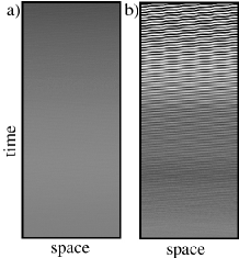
Figure 1: Spatio-temporal diagram of the electric field of the semiclassical model (equation (6)) with $L=120$, $\delta=0.94$, $g=0.6$, $D_{o}=0.0338$ a) without dissipation $\kappa=\gamma_{\perp}=\gamma_{\parallel}=0$, b) with dissipation $\kappa=0.03$, $\gamma_{\perp}=0.01$, $\gamma_{\parallel}=0.03$ and $N_{o}=0.0338$.

Figure 1 shows the space-time diagram of the electric field of a numerical simulation of the semiclassical model, plus noise with small intensity, close to the 1:1 resonance without dissipative terms (see fig. 1a) and with dissipative ones (see Fig. 1b). The numerical simulations start with the same initial condition, namely, the no-lasing solution with excited atoms ($D_{0}>0$). It is clear from these pictures that the inclusion of dissipation induces the Laser to respond. One can physically understand what happens, since without dissipation the atoms excited decay through the stimulated emission, i.e., the non-lasing solution becomes unstable very slowly (nonlinear mechanism). Instead, when one takes into account the dissipative terms, the excited atoms decay, for instance through stimulated emission and collisions, i.e., exponentially in time. Note that, one must to pump to $N_{0}=D_{0}$ in order that the non-lasing solution persists. In brief, with nonzero detuning and slight pumping, the dissipation induces the Laser to respond.

To illustrate the 1:1 resonance in a simple Hamiltonian system, we consider a mechanical system, that we call the Mechanical Laser, which consists of two coupled spherical pendula in a gravitational field, with a support, which can rotate around a vertical axis. The lower pendulum is constrained to move in a plane that is orthogonal to the plane of the upper pendulum (see Fig. 2).

The system rotates with angular velocity $\dot{\varphi}$ with respect to the vertical. The quantities $m_{1}$, $m_{2}$, $l_{1}$ and $l_{2}$ are the mass and length of the upper and lower pendula respectively, and $I$ is the dimensionless moment of inertia of the support. The system will dissipate energy because of friction at the contacts and the motion of the pendulum masses in a fluid (for example, the air) via Stokes’ law. Energy is injected through a constant torque at the upper pendulum pivot point. The governing equations for the angles $\theta_{1}\left(t\right)$ and $\theta_{2}\left(t\right)$ and the vertical angular velocity $\dot{\varphi}$ read Clerc2001

$$\ddot{\theta}_{1}=-\sigma^{2}\sin\theta_{1}\sin\theta_{2}\ddot{\theta}_{2}-\sigma^{2}\sin\theta_{1}\cos\theta_{2}\dot{\theta}_{2}^{2}$$

$$-2\sigma^{2}\cos\theta_{1}\cos\theta_{2}\dot{\varphi}\dot{\theta}_{2}+\sin\theta_{1}\cos\theta_{1}\dot{\varphi}^{2}$$

$$-\sigma^{2}\cos\theta_{1}\sin\theta_{2}\ddot{\varphi}-\frac{g}{l}\sin\theta_{1}-\nu_{1}\dot{\theta}_{1},$$

$$\ddot{\theta}_{2}=-\sin\theta_{1}\sin\theta_{2}\ddot{\theta}_{1}-\cos\theta_{1}\sin\theta_{2}\dot{\theta}_{1}^{2}$$

$$+2\cos\theta_{1}\cos\theta_{2}\dot{\varphi}\dot{\theta}_{1}+\sin\theta_{2}\cos\theta_{2}\dot{\varphi}^{2}$$

$$+\sin\theta_{1}\cos\theta_{2}\ddot{\varphi}-\frac{g}{l}\sin\theta_{2}-\nu_{2}\dot{\theta}_{2},$$

$$\frac{d}{dt}\left\{\begin{array}[]{c}\left(\sin^{2}\theta_{1}+\sigma^{2}\sin^{2}\theta_{2}\right)\dot{\varphi}+\sigma^{2}\cos\theta_{1}\sin\theta_{2}\dot{\theta}_{1}\\ -\sigma^{2}\sin\theta_{1}\cos\theta_{2}\dot{\theta}_{2}+I\dot{\varphi}\end{array}\right\}$$

$$=-\nu_{\varphi}\left(\dot{\varphi}-\Omega\right)-\mu_{1}\sin^{2}\theta_{1}\dot{\varphi}-\mu_{2}\left(\sin^{2}\theta_{1}+\sin^{2}\theta_{2}\right)\dot{\varphi}.$$

where $\nu_{1}$, $\nu_{2}$, $\nu_{\varphi}$, $\mu_{1}$ and $\mu_{2}$ are damping coefficients, $\sigma=\sqrt{m_{2}/\left(m_{1}+m_{2}\right)}$ is the relative factor of the energy between the oscillators, and we have written the torque as $\nu_{\varphi}\Omega$. For the sake of simplicity, we have considered the case of pendula of equal lengths ($l_{1}=l_{2}=l$). When one regards the Hamiltonian limit of the previous equations, the vertical solution or non-lasing solution $\theta_{1}=\theta_{2}=0$, $\dot{\varphi}=\Omega_{0}$ has a 1:1 resonance when

$$\Omega_{0}=\Omega_{c}=\sqrt{\frac{g}{l}\frac{\left(m_{1}+m_{2}\right)}{m_{1}}}$$

with frequency $\omega_{c}=\pm\sqrt{gm_{2}/lm_{1}}$. The centripetal force is more intense than the gravitational force when $\Omega_{0}\geq\Omega_{g}\equiv\sqrt{g/l}$. As a consequence, the Coriolis force exerted by one pendulum on the other, the non-lasing solution is marginal when $\Omega_{g}\leq\Omega_{0}\leq\Omega_{c}$. In this region the system is nonlinearly unstable and the system becomes linearly unstable when $\Omega_{0}>\Omega_{c}$; this exhibits a coherence oscillation, which is the signatures of the laser instability.

Near the 1:1 resonance, the coupled pendulum is govern by (5), whereClerc2001

$$\varepsilon = 2\frac{g}{l}\frac{\left(\Omega-\Omega_{c}\right)}{\Omega_{c}},\text{\ }\alpha=\frac{g}{4l}\left(\frac{\sigma^{4}-2\sigma^{3}-2\sigma^{2}+3}{1-\sigma^{2}}\right),$$

$$\delta = 2\sigma\left(\Omega-\Omega_{c}\right),\text{\ }\nu=\frac{\nu_{\varphi}}{I},\text{ \ }\mu=\frac{1}{2l^{2}}\left(\nu_{1}+\nu_{2}\right),$$

$$\eta = \frac{1}{I}\left[\mu_{1}+\left(1+\frac{1}{\sigma^{2}}\right)\mu_{2}-2\frac{\nu_{\varphi}}{\sigma^{2}I}\left(\frac{\Omega}{\Omega_{c}}-1\right)\right];$$

where the variables are related to the dominate order by $A=\left(\sigma\theta_{1}+i\theta_{2}\right)\exp(i\omega_{c}t)/2$ and $Z=2\Omega_{c}\sigma^{2}\left(\Omega_{c}-\dot{\varphi}\right)$. Transforming equations (5) to the Maxwell-Bloch equations, one obtains the following analogy of the electric field, polarization and population inversion

$$E = \frac{\left\{\sigma\theta_{1}+i\theta_{2}\right\}}{2}e^{i\left(\Delta+\omega_{c}\right)t}+c.c.$$

$$P = \frac{\left\{\sigma\dot{\theta}_{1}+i\dot{\theta}_{2}+a\left(\sigma\theta_{1}+i\theta_{2}\right)\right\}}{2}e^{i\left(\Delta+\omega_{c}\right)t}+c.c.$$

$$N = \frac{2\Omega_{c}\sigma^{2}}{\alpha}\left(\dot{\varphi}-\Omega_{c}\right)+\varepsilon_{0}-\frac{\sigma^{2}\theta_{1}^{2}+\theta_{2}^{2}}{4}$$

where $\Delta=\delta\left(\nu\alpha+\eta\right)/\left(2\nu\alpha+2\eta-\mu\alpha\right),$ $a=\left(\nu\alpha+\eta\right)/\alpha+i2\Delta$ and $\varepsilon_{0}=\left(\varepsilon+\Delta^{2}-\delta\Delta\right)/\alpha+\left(\nu\alpha+\eta\right)(\mu\alpha-\nu\alpha-\eta)/\alpha^{3}.$ The mechanical analog of the electric field is a simple function of the pendulum displacements with respect to the vertical. In the Hamiltonian case the polarization is the slow time derivative of the electric field. The mechanical analogy of the stimulated emission mechanism (time reversal effect) is the vertical angular momentum conservation. Thus, when one increases the pendula tilt (the intensity of the electric field enlargement), the angular velocity decreases (the population inversion declines). This is a main ingredient of Laser theory. If the torque or pumping is bigger than the gravitational force ($\Omega_{0}>\Omega_{g}$), i.e., the system is excited in Laser terminology, then the torque that gives rise to an angular velocity slightly higher than $\Omega_{g}$ leads to a dissipation induced instability.

In summary, we have studied the 1:1 resonance for perturbed Hamiltonian systems with small dissipative and energy injection terms. Nearby, the 1:1 resonance exhibits dissipation induces instabilities. This allow us to show that a slightly pumping optical cavity is unstable when one takes into account the dissipative effects. The Maxwell-Bloch equations are the asymptotic normal form that describe this instability when energy is injected through forcing at zero frequency. We have displayed a simple mechanical system, the Mechanical laser or double spherical pendulum with a support, which, close to the 1:1 resonance, is a mechanical analog of the Laser.

We thank Richard Murray for his encouragement and help in making this work possible and CDS for its hospitality. JEM was partially supported by the National Science Foundation.

Figure 2: Schematic representation of the Mechanical Laser.

References

- (1) R. Abraham and J.E. Marsden, Foundations of mechanics. (Addison-Wesley, Massachusetts, 1978).
- (2) J.E. Marsden and T. S. Ratiu, Introduction to Mechanics and Symmetry (Springer-Verlag, New York, 1994).
- (3) W. Thomson and P.G. Tait, Principles of Mechanics and Dynamics, Cambridge University Press (1897). Reprinted by Dover Publications, New York1962).
- (4) Y. Rocard, L’instabilité en Mécanique (Masson et cie., Paris, 1954).
- (5) J.D. Gibbon and M. McGuinness, Phys. Lett. A 77, 295(1980).
- (6) M. Clerc, P. Coullet and E. Tirapegui, Phys. Rev. Lett. 83, 3820 (1999).
- (7) M. Clerc, P. Coullet and E. Tirapegui, Optical Communication 166, 159 (1999).
- (8) M. Sargent, M. O. Scully, and W. E. Lamb, Laser Physics (Addison-Wesley, Massachusetts, 1974).
- (9) A.M. Bloch, P.S. Krishnaprasad, J.E. Marsden and T. S. Ratiu, Ann. I.H. Poincaré-an 11, 37 (1994).
- (10) C. Elphick, E. Tirapegui , M. Brachet, P. Coullet, G. Iooss , Physica D 29, 95 (1987).
- (11) J. Pedlosky, J. Atmos.Sci. 28, 587 (1971).
- (12) M. Weissman, Phil. Trans. R. Soc. London A 290, 639 (1979).
- (13) A. E. Seigman, Laser (University Science books, Mill Valley,1986).
- (14) D.D Holm and G.Kovacic, Physica D 56, 270 (1992).
- (15) M. Clerc and J.E. Marsden, In preparation.