SUBMITTED TO: Journal of Physics A Variational Principles for Lagrangian Averaged Fluid Dynamics

Abstract

The Lagrangian average (LA) of the ideal fluid equations preserves their transport structure. This transport structure is responsible for the Kelvin circulation theorem of the LA flow and, hence, for its convection of potential vorticity and its conservation of helicity.

Lagrangian averaging also preserves the Euler-Poincaré (EP) variational framework that implies the LA fluid equations. This is expressed in the Lagrangian-averaged Euler-Poincaré (LAEP) theorem proven here and illustrated for the Lagrangian average Euler (LAE) equations.

PACS numbers: 02.40.-k, 11.10.Ef, 45.20.Jj, 47.10.+g

Keywords: Fluid dynamics, Variational principles, Lagrangian average

1 Introduction

Decomposition of multiscale problems and scale-up

In turbulence, in climate modeling and in other multiscale fluids problems, a major challenge is “scale-up.” This is the challenge of deriving models that correctly capture the mean, or large scale flow – including the influence on it of the rapid, or small scale dynamics.

In classical mechanics this sort of problem has been approached by choosing a proper “slow + fast” decomposition and deriving evolution equations for the slow mean quantities by using, say, the standard method of averages. For nondissipative systems in classical mechanics that arise from Hamilton’s variational principle, the method of averages may extend to the averaged Lagrangian method, under certain conditions.

Eulerian vs Lagrangian means

In meteorology and oceanography, the averaging approach has a venerable history and many facets. Often this averaging is applied in the geosciences in combination with additional approximations involving force balances (for example, geostrophic and hydrostatic balances). It is also sometimes discussed as an initialization procedure that seeks a nearby invariant “slow manifold.” Moreover, in meteorology and oceanography, the averaging may be performed in either the Eulerian, or the Lagrangian description. The relation between averaged quantities in the Eulerian and Lagrangian descriptions is one of the classical problems of fluid dynamics.

Generalized Lagrangian mean (GLM)

The GLM equations of Andrews and McIntyre [1978a] systematize the approach to Lagrangian fluid modeling by introducing a slow + fast decomposition of the Lagrangian particle trajectory in general form. In these equations, the Lagrangian mean of a fluid quantity evaluated at the mean particle position is related to its Eulerian mean, evaluated at the displaced fluctuating position. The GLM equations are expressed directly in the Eulerian representation. The Lagrangian mean has the advantage of preserving the fundamental transport structure of fluid dynamics. In particular, the Lagrangian mean commutes with the scalar advection operator and it preserves the Kelvin circulation property of the fluid motion equation.

Compatibility of averaging and reduction of Lagrangians for mechanics on Lie groups

In making slow + fast decompositions and constructing averaged Lagrangians for fluid dynamics, care must generally be taken to see that the averaging and reduction procedures do not interfere with each other. Reduction in the fluid context refers to symmetry reduction of the action principle by the subgroup of the diffeomorphisms that takes the Lagrangian representation to the Eulerian representation of the flow field. The theory for this yields the Euler-Poincaré (EP) equations, see Holm, Marsden and Ratiu [1998a,b] and Marsden and Ratiu [1999].

Lagrangian averaged Euler-Poincaré (LAEP) equations

The compatibility requirement between averaging and reduction is handled automatically in the Lagrangian averaging (LA) approach. The Lagrangian mean of the action principle for fluids does not interfere with its reduction to the Eulerian representation, since the averaging process is performed at fixed Lagrangian coordinate. Thus, the process of taking the Lagrangian mean is compatible with reduction by the particle-relabeling group of symmetries for Eulerian fluid dynamics.

In this paper, we perform this reduction of the action principle and thereby place the LA fluid equations such as GLM theory into the EP framework. In doing this, we demonstrate the variational reduction property of the Lagrangian mean. This is encapsulated in the LAEP Theorem proven here:

Theorem 1.1 (Lagrangian Averaged Euler-Poincaré Theorem)

The Lagrangian averaging process preserves the variational structure of the Euler-Poincaré framework.

According to this theorem, the Lagrangian mean’s preservation of the fundamental transport structure of fluid dynamics also extends to preserving the EP variational structure of these equations. This preservation of structure may be visualized as a cube in Figure 1. As we shall explain, the LAEP theorem produces a cube consisting of four equivalence relations on each of its left and right faces, and four commuting diagrams (one on each of its four remaining faces).

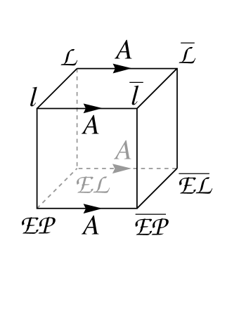
Figure 1: The Averaged EP theorem produces a cube consisting of four equivalence relations on each of its left and right faces, and four commuting diagrams (one on each of its four remaining faces).

Euler-Lagrange-Poincaré (ELP) cube

The front and back faces of the ELP cube live in the Eulerian (spatial) and Lagrangian (material) pictures of fluid dynamics, respectively. The top face contains four variational principles at its corners and the bottom face contains their corresponding equations of motion. The horizontal edges represent Lagrangian averaging and are directed from the left to the right. The left face contains the four equivalence relations of the Euler-Poincaré Theorem on its corners and the right face contains the corresponding averaged equivalence relations. Thus, the left and right faces of the ELP cube are equivalence relations, and its front, back, top and bottom faces are commuting diagrams.

The back face of the ELP cube displays the LA preservation of variational structure in the Lagrangian fluid picture. Hamilton’s principle with $L$ yields the Euler-Lagrange equations $EL$ in this picture, and Lagrangian averaging $A$ preserves this relation. Namely, Hamilton’s principle with the averaged Lagrangian $\bar{L}$ yields the averaged Euler-Lagrange equations $\overline{EL}$.

This pair of Hamilton’s principles and Euler-Lagrange equations has its counterpart in the Eulerian picture of fluid dynamics on the front face of the ELP cube – whose variational relations are also exactly preserved by the LA process.

The bottom front edge of the cube represents the GLM equations of Andrews and McIntyre [1978a]. Thus, the GLM equations represent a foundational result for the present theory.

The six faces of the ELP cube represent six interlocking equivalence relations and commutative diagrams that enable modeling and Lagrangian averaging to be performed equivalently either at the level of the equations, as in Andrews and McIntyre [1978a], or at the level of Hamilton’s principle. At the level of Hamilton’s principle, powerful theorems from other mean field theories are available. An example is Noether’s theorem, which relates symmetries of Hamilton’s principle to conservation laws of the equations of motion. Fluid conservation laws include mass, momentum and energy, as well as local conservation of potential vorticity. The latter yields the Casimirs of the corresponding Lie-Poisson Hamiltonian formulation of ideal fluid dynamics and is due to the symmetry of relabeling diffeomorphisms admitted by Hamilton’s principle for fluid dynamics, see Arnold [1966] and Holm, Marsden, Ratiu and Weinstein [1985]. In certain cases, the fluid vorticity winding number (called helicity – a topological quantity) is also conserved. Lagrangian averaging preserves all of these conservation laws. Thus, the LA Hamilton’s principle yields the LA fluid equations in either the Lagrangian, or the Eulerian fluid picture, and one may transform interchangeably along the edges of the cube in search of physical and mathematical insight.

Remark 1.2 (Eulerian mean)

Of course, the preservation of variational structure resulting in the interlocking commuting relationships and conservation laws of the LAEP Theorem is not possible with the Eulerian mean, because the Eulerian mean does not preserve the transport structure of fluid mechanics.

Remark 1.3 (Balanced approaches)

The LAEP Theorem puts the approach using averaged Hamilton’s principles and the method of Lagrangian averaged equations onto equal footing. This is quite a bonus for both approaches to modeling fluids. According to the LAEP Theorem, the averaged Hamilton’s principle produces dynamics that is guaranteed to be verified directly by averaging the original equations, and the Lagrangian averaged equations inherit the conservation laws that are available from the symmetries of Hamilton’s principle.

Outline of the paper

In section 2, we begin by briefly reviewing the mathematical setting of the EP theorem from Holm, Marsden and Ratiu [1998a,b]. We state the EP theorem and discuss a few of its implications for continuum mechanics in vector notation. We also sketch its proof, in preparation for proving the corresponding results for the Lagrangian Averaged Euler-Poincaré (LAEP) theorem presented in section 3. Finally, in section 4, we illustrate the LAEP theorem by applying it to incompressible ideal fluids. We also mention recent progress toward closure of these equations as models of fluid turbulence.

2 The Euler-Poincaré theorem for fluids with advected properties

2.1 Mathematical setting and statement of the EP theorem

The assumptions of the Euler-Poincaré theorem from Holm, Marsden and Ratiu [1998a] are briefly listed below.

$\quad\bullet$ There is a right representation of Lie group $G$ on the vector space $V$ and $G$ acts in the natural way on the right on $TG\times V^{\ast}$: $(v_{g},a)h=(v_{g}h,ah)$.

$\quad\bullet$ Assume that the function $L:TG\times V^{\ast}\rightarrow\mathbf{R}$ is right $G$–invariant.

$\quad\bullet$ In particular, if $a_{0}\in V^{\ast}$, define the Lagrangian $L_{a_{0}}:TG\rightarrow\mathbf{R}$ by $L_{a_{0}}(v_{g})=L(v_{g},a_{0})$. Then $L_{a_{0}}$ is right invariant under the lift to $TG$ of the right action of $G_{a_{0}}$ on $G$, where $G_{a_{0}}$ is the isotropy group of $a_{0}$.

$\quad\bullet$ Right $G$–invariance of $L$ permits one to define $\ell:{\mathbf{g}}\times V^{\ast}\rightarrow\mathbf{R}$ by

$$\ell(v_{g}g^{-1},a_{0}g^{-1})=L(v_{g},a_{0}).$$

Conversely, this relation defines for any $\ell:{\mathbf{g}}\times V^{\ast}\rightarrow\mathbf{R}$ a right $G$–invariant function $L:TG\times V^{\ast}\rightarrow\mathbf{R}$.

$\quad\bullet$ For a curve $g(t)\in G,$ let

$$u(t)\equiv\dot{g}(t)g(t)^{-1}\in TG/G\cong\mathbf{g}$$

and define the curve $a(t)$ as the unique solution of the linear differential equation with time dependent coefficients

$$\dot{a}(t)=-a(t)u(t)$$ (2.1)

where the action of $u\in\mathbf{g}$ on the initial condition $a(0)=a_{0}\in V^{*}$ is denoted by concatenation from the right. The solution of (2.1) can be written as the advective transport relation,

$$a(t)=a_{0}g(t)^{-1}\,.$$

Theorem 2.1 (EP Theorem)

The following are equivalent:

1. Hamilton’s variational principle

   $$\delta\int_{t_{1}}^{t_{2}}L_{a_{0}}(g(t),\dot{g}(t))dt=0$$ (2.2)

   holds, for variations $\delta g(t)$ of $g(t)$ vanishing at the endpoints.

2. $g(t)$ satisfies the Euler–Lagrange equations for $L_{a_{0}}$ on $G$.

3. The constrained variational principle

   $$\delta\int_{t_{1}}^{t_{2}}\ell\,(u(t),a(t))dt=0$$ (2.3)

   holds on $\mathbf{g}\times V^{\ast}$, using variations of the form

   $$\delta u=\frac{\partial\eta}{\partial t}+{\rm ad}_{u}\,\eta,\quad\delta a=-a\,\eta,$$ (2.4)

   where $\eta(t)\in\mathbf{g}$ vanishes at the endpoints.

4. The Euler–Poincaré equations hold on $\mathbf{g}\times V^{\ast}$

   $$\frac{\partial}{\partial t}\frac{\delta\ell}{\delta u}=-{\rm ad}_{u}^{\ast}\frac{\delta\ell}{\delta u}+\frac{\delta\ell}{\delta a}\diamond a.$$ (2.5)

2.2 Discussion of the EP equations in vector notation

When mass is the only advected quantity, the EP motion equation (2.5) and the advection relation (2.1) for mass conservation are written as

$$\Big{(}\frac{\partial}{\partial t}+{\rm ad}^{*}_{u}\Big{)}\frac{\delta\ell}{\delta{u}}-\frac{\delta\ell}{\delta{D}}\diamond D=0\,,\quad\hbox{and}\quad\frac{\partial D}{\partial t}=-\,\pounds_{u}D\,.$$

Here $\pounds_{u}$ denotes the Lie derivative with respect to velocity ${u}$, and the operations ad^∗ and $\diamond$ are defined using the $L_{2}$ pairing $\langle{f,g}\rangle=\int fg\,d^{3}x$. The ad^∗ operation is defined as (minus) the $L_{2}$ dual of the Lie algebra operation, ad, for vector fields, namely

$$-\,\Big{\langle}{\rm ad}^{*}_{u}\,\frac{\delta\ell}{\delta{u}},\eta\Big{\rangle}=\Big{\langle}\frac{\delta\ell}{\delta{u}},{\rm ad}_{u}\,\eta\Big{\rangle}\,.$$

In vector notation ad${}_{u}\,\eta$ is expressed as

$${\rm ad}_{u}\,\eta=\eta u-u\eta=-\,[u,\eta\,]=-\,{\rm ad}_{\eta}\,u=u\cdot\nabla\eta-\eta\cdot\nabla u\,.$$

The diamond operation $\diamond$ is defined as (minus) the $L_{2}$ dual of the Lie derivative, namely,

$$-\,\Big{\langle}\frac{\delta\ell}{\delta a}\diamond a,\eta\Big{\rangle}=\Big{\langle}\frac{\delta\ell}{\delta a},\pounds_{\eta}a\Big{\rangle}\,.$$

Here $a$ and $\delta\ell/\delta a$ are dual tensors and $(\delta\ell/\delta a)\diamond a$ is a one-form density (dual to vector fields under $L_{2}$ pairing). In vector notation the diamond operation $\diamond$ for the example of the density $D$ becomes

$$-\,\Big{\langle}\frac{\delta\ell}{\delta{D}}\diamond D,\eta\Big{\rangle}=\Big{\langle}\frac{\delta\ell}{\delta{D}},\pounds_{\eta}D\Big{\rangle}=\Big{\langle}\frac{\delta\ell}{\delta{D}},{\rm div}(D\eta)\Big{\rangle}=-\,\Big{\langle}D\nabla\frac{\delta\ell}{\delta{D}},\eta\Big{\rangle}\,.$$

Thus, the EP motion equation (2.5) may be written in Cartesian components as

$$\frac{\partial}{\partial t}\frac{\delta\ell}{\delta{u}^{i}}+\underbrace{\,\frac{\partial}{\partial{x}^{j}}\Big{(}\frac{\delta\ell}{\delta{u}^{i}}{u}^{j}\Big{)}+\frac{\delta\ell}{\delta u^{j}}\frac{\partial{u}^{j}}{\partial{x}^{i}}}_{\equiv\,\big{(}{\rm ad}^{*}_{u}\,\frac{\delta\ell}{\delta{u}}\big{)}_{i}\,}-\underbrace{\,D\frac{\partial}{\partial{x}^{i}}\Big{(}\frac{\delta\ell}{\delta{D}}\Big{)}\,}_{\equiv\,\big{(}\frac{\delta\ell}{\delta{D}}\,\diamond\,D\big{)}_{i}}=0\,,$$

and the advection relation for the mass density $D\in V^{*}$ satisfies,

$$\Big{(}\frac{\partial}{\partial t}+\pounds_{u}\Big{)}\Big{(}D\,d^{3}x\Big{)}=0\,,\quad\hbox{or}\quad\frac{\partial D}{\partial t}=-\,{\rm div}(D\mathbf{u})\,.$$

Remarks.

$\quad\bullet$ In passing from coordinate-free forms to their component expressions, we shall write tensors in a Cartesian basis. For example, we shall include the volume form in the mass density by denoting it as $Dd^{3}x$.

$\quad\bullet$ The EP motion equation and mass advection equation may also be written equivalently using Lie derivative notation as

$$\Big{(}\frac{\partial}{\partial t}+\pounds_{u}\Big{)}\frac{\delta\ell}{\delta{u}}-\frac{\delta\ell}{\delta{D}}\diamond D=0\,,\quad\hbox{and}\quad\Big{(}\frac{\partial}{\partial t}+\pounds_{u}\Big{)}D=0\,.$$

The equivalence here of $\pounds_{u}$ and ad${}^{*}_{u}$ arises because $\delta\ell/\delta u$ is a one-form density and the equality ad${}^{*}_{u}\mu=\pounds_{u}\mu$ holds for any one-form density $\mu$.

$\quad\bullet$ In the Lie derivative notation, one proves the Kelvin-Noether circulation theorem immediately as a corollary, by

$$\frac{d}{dt}\oint_{c(u)}\frac{1}{D}\ \frac{\delta\ell}{\delta{u}}=\oint_{c(u)}\!\!\Big{(}\frac{\partial}{\partial t}+\pounds_{u}\Big{)}\frac{1}{D}\ \frac{\delta\ell}{\delta{u}}=\oint_{c(u)}\frac{1}{D}\ \frac{\delta\ell}{\delta{D}}\diamond D\,,$$

for any closed curve $c(u)$ that moves with the fluid. In vector notation, this is seen as

$$\frac{d}{dt}\oint_{c(u)}\frac{1}{D}\ \frac{\delta\ell}{\delta\mathbf{u}}\cdot d\mathbf{x}=\oint_{c(u)}\nabla\frac{\delta\ell}{\delta{D}}\cdot d\mathbf{x}=0\,.$$ (2.6)

$\quad\bullet$ Helicity conservation. In Lie derivative notation, one may rewrite the Kelvin circulation theorem as

$$\Big{(}\frac{\partial}{\partial t}+\pounds_{u}\Big{)}v+dp=0\,,$$

where

$$v=\mathbf{v}\cdot d\mathbf{x}=\frac{1}{D}\ \frac{\delta\ell}{\delta\mathbf{u}}\cdot d\mathbf{x}\,,\quad\hbox{and}\quad p=-\,\frac{\delta\ell}{\delta{D}}\,.$$

Therefore,

$$\Big{(}\frac{\partial}{\partial t}+\pounds_{u}\Big{)}(v\wedge dv)=-d\,(p\,dv)\,,$$

where $\wedge$ is the exterior product of differential forms. In vector notation, this is the helicity equation,

$$\frac{\partial}{\partial t}(\mathbf{v}\cdot{\rm curl}\,\mathbf{v})+{\rm div}\,\big{(}\mathbf{u}\,(\mathbf{v}\cdot{\rm curl}\,\mathbf{v})+p\ {\rm curl}\,\mathbf{v}\big{)}=0\,.$$ (2.7)

Consequently, for homogeneous boundary conditions one finds conservation of helicity $\Lambda=\int v\wedge dv=\int\mathbf{v}\cdot{\rm curl}\,\mathbf{v}\,d^{3}x$. The helicity $\Lambda$ is a topological quantity that measures the linkage number of the lines of curl$\,\mathbf{v}$, the fluid vortex lines in this case.

2.3 Proof of the EP Theorem

The equivalence of i and ii holds for any configuration manifold and so, in particular, it holds in this case.

The following string of equalities shows that iii is equivalent to iv.

$$0 = \delta\int_{t_{1}}^{t_{2}}\!\!\ell(u,a)\,dt=\int_{t_{1}}^{t_{2}}\Big{\langle}\frac{\delta\ell}{\delta u}\,,\,\delta u\Big{\rangle}+\Big{\langle}\frac{\delta\ell}{\delta a}\,,\,\delta a\Big{\rangle}\,dt$$ (2.8)

$$= \int_{t_{1}}^{t_{2}}\left\langle\frac{\delta\ell}{\delta u}\,,\,\frac{\partial\eta}{\partial t}+{\rm ad}_{u}\,\eta\right\rangle-\left\langle\frac{\delta\ell}{\delta a}\,,\,\pounds_{\eta}\,a\right\rangle\,dt$$

$$= -\int_{t_{1}}^{t_{2}}\left\langle\frac{\partial}{\partial t}\frac{\delta\ell}{\delta u}+{\rm ad}^{*}_{u}\frac{\delta\ell}{\delta u}-\frac{\delta\ell}{\delta a}\diamond a\,,\,\eta\right\rangle dt\,.$$

Finally we show that i and iii are equivalent. First note that the $G$–invariance of $L:TG\times V^{\ast}\rightarrow\mathbf{R}$ and the definition of $a(t)=a_{0}g(t)^{-1}$ imply that the integrands in (2.2) and (2.3) are equal. Moreover, all variations $\delta g(t)\in TG$ of $g(t)$ with fixed endpoints induce and are induced by variations $\delta u(t)\in\mathbf{g}$ of $u(t)$ of the form $\delta u=\partial\eta/\partial t+{\rm ad}_{u}\,\eta$ with $\eta(t)\in\mathbf{g}$ vanishing at the endpoints. The relation between $\delta g(t)$ and $\eta(t)$ is given by $\eta(t)=\delta g(t)g(t)^{-1}$. This is the proof first given in Holm, Marsden and Ratiu [1998a].

QED

3 Lagrangian averaged Euler-Poincaré theory

We shall place the GLM (Generalized Lagrangian Mean) theory of Andrews and McIntyre [1978a] into the Euler-Poincaré framework discussed in the previous section.

3.1 GLM theory from a geometric viewpoint

The GLM theory of Andrews and McIntyre [1978a] begins by assuming the Lagrange-to-Euler map factorizes as a product of diffeomorphisms,

$$g(t)=\Xi\,(t)\cdot\tilde{g}(t)\,.$$

Moreover, the first factor $\tilde{g}(t)$ arises from an averaging process,

$$\bar{g}(t)=\overline{\Xi\,(t)\cdot\tilde{g}(t)}=\tilde{g}(t)\,,$$

that satisfies the projection property, so that $\bar{\tilde{g}}(t)=\tilde{g}(t)$. Thus, a fluid parcel labeled by $\mathbf{x}_{0}$ has current position,

$$\mathbf{x}^{\xi}(\mathbf{x}_{0},t)\equiv\Xi\,(t)\cdot(\tilde{g}(t)\cdot\mathbf{x}_{0})=\Xi\,(\mathbf{x}(\mathbf{x}_{0},t),t)\quad\hbox{(current position)}\,,$$

and it has mean position,

$$\mathbf{x}(\mathbf{x}_{0},t)=\tilde{g}(t)\cdot\mathbf{x}_{0}\quad\hbox{(mean position)}\,.$$

Remark 3.1

Thus, GLM theory first averages the action of the diffeomorphism group, while holding fixed the material objects on which the group acts. Then it restores the original action of the group by assuming that $g(t)\cdot\tilde{g}^{-1}(t)=\Xi\,(t)$ is also a diffeomorphism. This is illustrated in Figure 2.

Figure 2: GLM theory factorizes the Lagrange to Euler map at a given time by first mapping the reference configuration to the mean position, then mapping that to the current position.

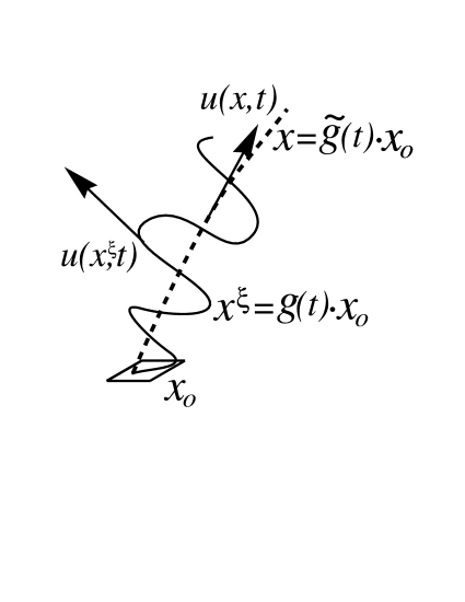
Figure 3: The GLM velocities $\mathbf{u}(\mathbf{x}^{\xi},t)$ and $\bar{\mathbf{u}}^{L}(\mathbf{x},t)$ are tangent to the current and mean trajectories, $\mathbf{x}^{\xi}$ and $\mathbf{x}$, respectively.

The composition of maps $g(t)=\Xi\,(t)\cdot\tilde{g}(t)$ yields via the chain rule the following velocity relation,

$$\dot{g}(t)\cdot\mathbf{x}_{0}=\dot{\Xi}\,(t)\cdot\mathbf{x}+T\Xi\cdot\!(\dot{\tilde{g}}(t)\cdot\mathbf{x}_{0})\,.$$ (3.1)

By invertibility, $\mathbf{x}_{0}=g^{-1}(t)\cdot\mathbf{x}^{\xi}=\tilde{g}^{-1}(t)\cdot\mathbf{x}$. Consequently, one may define the fluid parcel velocity at the current position in terms of a vector field evaluated at the mean position as,

$$\mathbf{u}(\mathbf{x}^{\xi},t)=\dot{g}\cdot g^{-1}(t)\cdot\mathbf{x}^{\xi}=\dot{g}\cdot\tilde{g}^{-1}(t)\cdot\mathbf{x}=\mathbf{u}^{\xi}(\mathbf{x},t)\,.$$

Hence, by using the velocity relation (3.1) one finds,

$$\mathbf{u}^{\xi}(\mathbf{x},t) = \dot{\Xi}\,(t)\cdot\mathbf{x}+T\Xi\cdot\!\big{(}\,\dot{\tilde{g}}\tilde{g}^{-1}(t)\cdot\mathbf{x}\,\big{)}$$ (3.2)

$$\equiv \frac{\partial\Xi}{\partial t}\,(\mathbf{x},t)+\frac{\partial\Xi}{\partial\mathbf{x}}\cdot\bar{\mathbf{u}}^{L}(\mathbf{x},t)\,.$$

Here the Lagrangian mean velocity $\bar{\mathbf{u}}^{L}$ is defined as

$$\bar{\mathbf{u}}^{L}(\mathbf{x},t)\equiv\overline{\mathbf{u}^{\xi}(\mathbf{x},t)}=\overline{\dot{g}\tilde{g}^{-1}(t)}\cdot\mathbf{x}=\dot{\tilde{g}}(t)\tilde{g}(t)^{-1}\cdot\mathbf{x}=\dot{\tilde{g}}(t)\cdot\mathbf{x}_{0}\,.$$ (3.3)

In the third equality we used the projection property of the averaging process and found $\overline{\dot{g}}=\dot{\overline{g}}=\dot{\tilde{g}}$ from equation (3.1), so that

$$\bar{\mathbf{u}}^{L}(\mathbf{x},t)=\dot{\tilde{g}}(t)\tilde{g}(t)^{-1}\cdot\mathbf{x}\equiv\tilde{\mathbf{u}}(\mathbf{x},t)\,.$$

Thus, the Lagrangian mean velocity vector satisfies $\bar{\mathbf{u}}^{L}=\tilde{\mathbf{u}}$, so $\bar{\mathbf{u}}^{L}$ is tangent to the mean motion associated with $\tilde{g}(t)$. Hence, one may write equation (3.2) in terms of the mean material time derivative $D^{L}/Dt$ as

$$\mathbf{u}^{\xi}(\mathbf{x},t)=\Big{(}\frac{\partial}{\partial t}+\bar{\mathbf{u}}^{L}\cdot\nabla\Big{)}\,\Xi(\mathbf{x},t)\equiv\frac{D^{L}}{Dt}\,\Xi\,(\mathbf{x},t)\,.$$ (3.4)

Likewise, for any fluid quantity $\chi$ one may define $\chi^{\xi}$ as the composition of functions

$$\chi^{\xi}(\mathbf{x},t)=\chi(\mathbf{x}^{\xi},t)=\chi(\Xi\,(\mathbf{x},t),t)\,.$$

Taking the mean material time derivative and using the definition of $D^{L}/Dt$ in equation (3.4) yields the advective derivative relation,

$$\frac{D^{L}}{Dt}\chi^{\xi} = \Big{(}\frac{\partial\chi}{\partial t}\Big{)}^{\xi}+T\chi\cdot\frac{D^{L}}{Dt}\Xi\,(\mathbf{x},t)$$ (3.5)

$$= \Big{(}\frac{\partial\chi}{\partial t}+T\chi\cdot\mathbf{u}\Big{)}^{\xi}\equiv\Big{(}\frac{D\chi}{Dt}\Big{)}^{\xi}\,.$$

As in equation (3.3) for the velocity, the Lagrangian mean $\bar{\chi}^{L}$ of any other fluid quantity $\chi$ is defined as

$$\bar{\chi}^{L}(\mathbf{x},t)\equiv\overline{\chi^{\xi}(\mathbf{x},t)}=\overline{\chi(\mathbf{x}^{\xi},t)}=\overline{\chi\big{(}\,\Xi\,(t)\cdot\mathbf{x},t\big{)}}=\overline{\chi\big{(}\,g(t)\cdot\mathbf{x}_{0},t\big{)}}\,.$$

Taking the Lagrangian mean of equation (3.5) and once again using its projection property yields

$$\dot{\bar{\chi}}^{L}=\frac{D^{L}}{Dt}\bar{\chi}^{L}=\overline{\Big{(}\frac{D\chi}{Dt}\Big{)}}^{L}=\bar{\dot{\chi}}^{L}\,,\quad\hbox{so that}\quad\frac{D^{L}}{Dt}\chi^{\ell}=\Big{(}\frac{D\chi}{Dt}\Big{)}^{\ell}\,,$$

where $\chi^{\ell}=\chi^{\xi}-\bar{\chi}^{L}$ is the Lagrangian disturbance of $\chi$ satisfying $\overline{\chi^{\ell}}=0$.

Remark 3.2

The Lagrangian mean commutes with the material derivative. Hence, the advective derivative relation (3.5) decomposes additively, as

$$\frac{D^{L}}{Dt}\Big{(}\chi^{L}+\chi^{\ell}\Big{)}=\overline{\Big{(}\frac{D\chi}{Dt}\Big{)}}^{L}+\Big{(}\frac{D\chi}{Dt}\Big{)}^{\ell}\,.$$ (3.6)

3.2 Mean advected quantities and their transformations

Advective transport by $g(t)$ and $\tilde{g}(t)$ is defined by

$$a(\mathbf{x}^{\xi},t)=a_{0}\cdot g^{-1}(t)\quad\hbox{and}\quad\tilde{a}(\mathbf{x},t)=a_{0}\cdot\tilde{g}^{-1}(t)\,,$$

where $a_{0}=a(\mathbf{x}_{0},0)=\tilde{a}(\mathbf{x}_{0},0)$, with $a,\tilde{a}\in V^{*}$ and the factorization $g(t)=\Xi\,(t)\cdot\tilde{g}(t)$ implies

$$\tilde{a}(\mathbf{x},t)=a\cdot\,\Xi\,(\mathbf{x},t)\,.$$

Note that the right side of this equation is potentially rapidly varying, but the left side is a mean advected quantity.

Since $a$ and $\tilde{a}$ refer to the same initial conditions, $a_{0}$, one finds

$$a_{0}\cdot\tilde{g}^{-1}(t)=\tilde{a}(\mathbf{x},t)=a\cdot\,\Xi\,(\mathbf{x},t)=a(\mathbf{x}^{\xi},t)\equiv{\cal F}(\mathbf{x},t)\cdot a^{\xi}(\mathbf{x},t)\,,$$ (3.7)

where ${\cal F}(\mathbf{x},t)$ is the tensor transformation factor of $a$ under the change of variables $\Xi\,:\mathbf{x}\to\mathbf{x}^{\xi}$. For example, one computes formula (3.7) for an advected density as

$$\Big{(}D(\mathbf{x}_{0})d^{3}x_{0}\Big{)}\cdot\tilde{g}^{-1}(t)=D^{\xi}(\mathbf{x},t)\det(T\Xi)\,d^{3}x=\tilde{D}(\mathbf{x},t)\,d^{3}x\,.$$ (3.8)

Thus, for an advected density, $D$,

$$D^{\xi}\det(T\Xi)(\mathbf{x},t)=\tilde{D}(\mathbf{x},t)\,,\quad{\cal F}(\mathbf{x},t)=\det(T\Xi)\,,\quad\frac{\partial}{\partial t}\tilde{D}=-\,{\rm div}\,(\tilde{D}\tilde{\mathbf{u}})\,.$$

For an advected scalar function, $s$,

$$s^{\xi}(\mathbf{x},t)=\tilde{s}(\mathbf{x},t)=\bar{s}^{L}(\mathbf{x},t)\,,\quad{\cal F}=1\,,\quad\frac{\partial}{\partial t}\tilde{s}=-\,\tilde{\mathbf{u}}\cdot\nabla\tilde{s}\,.$$

For an advected vector field, $\mathbf{B}$,

$$K^{i}_{j}\,{B}^{\xi\,j}(\mathbf{x},t)=\tilde{B}^{i}(\mathbf{x},t)\,,\quad\hbox{and}\quad K^{i}_{j}=\det(T\Xi\,)\,(T\Xi^{\,-1})^{i}_{j}\,.$$

Thus, in the case of an advected vector field, one has

$$\mathsf{K}\cdot\mathbf{B}^{\xi}(\mathbf{x},t)=\tilde{\mathbf{B}}(\mathbf{x},t)\,,\quad\hbox{with}\quad{\cal F}=\mathsf{K}\equiv\det(T\Xi\,)\,T\Xi^{\,-1}\,,$$

and an advection relation (e.g., a frozen-in magnetic field) given by

$$\frac{\partial}{\partial t}\tilde{\mathbf{B}}=-\,\tilde{\mathbf{u}}\cdot\nabla\tilde{\mathbf{B}}+\tilde{\mathbf{B}}\cdot\nabla\tilde{\mathbf{u}}\,.$$

Finally, for an advected symmetric tensor $S$ one finds

$$(T\Xi^{\,T}\cdot S^{\xi}\cdot T\Xi\,)_{ij}=\tilde{S}_{ij}\,,$$

whose advection relation is obtained as in the other cases.

In each case, the corresponding transformation factor ${\cal F}$ appears in a variational relation for an advected quantity, expressed via equation (3.7) as

$$\delta{a}^{\xi}=\delta\,({\cal F}^{-1}\cdot\tilde{a})={\cal F}^{-1}\cdot\delta\tilde{a}+(\delta{\cal F}^{-1})\cdot\tilde{a}\,.$$ (3.9)

This formula will be instrumental in establishing the main result.

3.3 Lagrangian Averaged Euler-Poincaré Theorem

Let the assumptions hold as listed previously for the EP Theorem 2.1 and assume the GLM factorization $g(t)=\Xi\,(t)\cdot\tilde{g}(t)$ with $\bar{g}(t)=\overline{\Xi\,(t)\cdot\tilde{g}(t)}$. Then,

Theorem 3.3 (LAEP Theorem)

The following are equivalent:

1. The averaged Hamilton’s principle holds

   $$\delta\int_{t_{1}}^{t_{2}}\overline{L_{a_{0}}(g(t),\dot{g}(t))}\,dt=0$$ (3.10)

   for variations $\delta g(t)$ of $g(t)$ vanishing at the endpoints.

2. The mean Euler–Lagrange equations for $\bar{L}_{a_{0}}$ are satisfied on $\tilde{G}$,

   $$\overline{\frac{\delta L_{a_{0}}}{\delta{g}}\cdot T\Xi\,}-\overline{\frac{d}{dt}\frac{\delta L_{a_{0}}}{\delta\dot{g}}\cdot T\Xi}=0$$ (3.11)

3. The averaged constrained variational principle

   $$\delta\int_{t_{1}}^{t_{2}}\overline{\ell\,\big{(}u^{\xi}(t),a^{\xi}(t)\big{)}}dt=0$$ (3.12)

   holds on $\tilde{\mathbf{g}}\times\tilde{V}^{\ast}$, using variational relations of the form

   $$\delta u^{\xi}\!\! = \!\!T\Xi\,\cdot\!\Big{(}\frac{\partial\tilde{\eta}}{\partial t}+{\rm ad}_{\tilde{u}}\,\tilde{\eta}\Big{)}+\delta\,\Xi\hbox{ terms}\,,$$

   $$\delta a^{\xi}\!\! = \!\!{\cal F}^{-1}\!\cdot\delta\tilde{a}+\delta\,\Xi\hbox{ terms, and }\delta\tilde{a}=-\,\tilde{a}\,\tilde{\eta},$$

   where $\tilde{\eta}(t)=\delta\tilde{g}\,\tilde{g}^{-1}\in\tilde{\mathbf{g}}$ vanishes at the endpoints.

4. The Lagrangian averaged Euler–Poincaré (LAEP) equations hold on $\tilde{\mathbf{g}}\times\tilde{V}^{\ast}$

   $$\frac{\partial}{\partial t}\overline{\Big{(}\frac{\delta\ell}{\delta u^{\xi}}\cdot T\Xi\Big{)}}=-{\rm ad}_{\tilde{u}}^{\ast}\overline{\Big{(}\frac{\delta\ell}{\delta u^{\xi}}\cdot T\Xi\Big{)}}+\overline{\Big{(}\frac{\delta\ell}{\delta a^{\xi}}\cdot{\cal F}^{-1}\Big{)}}\diamond\tilde{a}\,.$$ (3.13)

Corollary 3.4 (LA Kelvin-Noether Circulation Theorem)

$$\frac{d}{dt}\oint_{c(\tilde{u})}\frac{1}{\tilde{D}}\ \overline{\Big{(}\frac{\delta\ell}{\delta u^{\xi}}\cdot T\Xi\Big{)}}=\oint_{c(\tilde{u})}\frac{1}{\tilde{D}}\ \overline{\Big{(}\frac{\delta\ell}{\delta a^{\xi}}\cdot{\cal F}^{-1}\Big{)}}\diamond\tilde{a}\,,$$

for any closed curve $c(\tilde{u})$ that moves with the fluid.

Proof. Via the equivalence of ad^∗ and Lie derivative for a one-form density, the (LAEP) equation implies

$$\frac{d}{dt}\oint_{c(\tilde{u})}\frac{1}{\tilde{D}}\ \overline{\Big{(}\frac{\delta\ell}{\delta u^{\xi}}\cdot T\Xi\Big{)}}=\oint_{c(\tilde{u})}\!\!\Big{(}\frac{\partial}{\partial t}+\pounds_{u}\Big{)}\frac{1}{\tilde{D}}\ \overline{\Big{(}\frac{\delta\ell}{\delta u^{\xi}}\cdot T\Xi\Big{)}}\,,$$

for any closed curve $c(\tilde{u})$ that moves with the fluid.

QED

3.4 Proof of the LAEP Theorem

The equivalence of $\overline{\bf i}$ and $\overline{\bf ii}$ holds for any configuration manifold and so, in particular, it holds again in this case. To compute the averaged Euler-Lagrange equation (3.11), we use the following variational relation obtained from the composition of maps $g(t)=\Xi\,(t)\cdot\tilde{g}(t)$, cf. the velocity relation (3.1),

$$\delta{g}(t)=\delta{\Xi}\,(t)\cdot\tilde{g}(t)+T\Xi\,(t)\cdot\delta\tilde{g}(t)\,.$$ (3.14)

Hence, we find

$$0 = \delta\int_{t_{1}}^{t_{2}}\overline{L_{a_{0}}(g(t),\dot{g}(t))}\,dt$$

$$= \int_{t_{1}}^{t_{2}}\bigg{(}\ \overline{\frac{\delta L_{a_{0}}}{\delta{g}}\cdot\delta{g}}+\overline{\frac{\delta L_{a_{0}}}{\delta\dot{g}}\cdot\delta\dot{g}}\ \bigg{)}\,dt$$

$$= \int_{t_{1}}^{t_{2}}\bigg{(}\ \overline{\frac{\delta L_{a_{0}}}{\delta{g}}\cdot T\Xi\,}-\overline{\frac{d}{dt}\frac{\delta L_{a_{0}}}{\delta\dot{g}}\cdot T\Xi}\ \bigg{)}\cdot\delta\tilde{g}\,dt\,.$$

This yields the mean Euler-Lagrange equations (3.11). Here we have dropped $\delta\,\Xi-$terms, because they do not figure in the variational principle for Lagrangian mean fluid dynamics at this level of description.

The following string of equalities shows that $\overline{\bf iii}$ is equivalent to $\overline{\bf iv}$.

$$0 = \delta\int_{t_{1}}^{t_{2}}\overline{\ell(u^{\xi},a^{\xi})}\,dt=\int_{t_{1}}^{t_{2}}\Big{\langle}\overline{\frac{\delta\ell}{\delta u^{\xi}}\,,\,\delta u^{\xi}}\Big{\rangle}+\Big{\langle}\overline{\frac{\delta\ell}{\delta a^{\xi}}\,,\,\delta a^{\xi}}\Big{\rangle}\,dt$$

$$= \int_{t_{1}}^{t_{2}}\Big{\langle}\overline{\frac{\delta\ell}{\delta u^{\xi}}\,,\,T\Xi\,\cdot\delta(\dot{\tilde{g}}\tilde{g}^{-1})}\Big{\rangle}+\Big{\langle}\overline{\frac{\delta\ell}{\delta a^{\xi}}\,,\,{\cal F}^{-1}\!\cdot\delta\tilde{a}}\Big{\rangle}\,dt$$

$$= \int_{t_{1}}^{t_{2}}\left\langle\ \overline{\frac{\delta\ell}{\delta u^{\xi}}\cdot T\Xi}\,,\,\frac{\partial\tilde{\eta}}{\partial t}+{\rm ad}_{\tilde{u}}\,\tilde{\eta}\right\rangle-\left\langle\ \overline{\frac{\delta\ell}{\delta a^{\xi}}\cdot{\cal F}^{-1}}\,,\,\pounds_{\tilde{\eta}}\,\tilde{a}\right\rangle\,dt$$

$$=-\int_{t_{1}}^{t_{2}}\left\langle\frac{\partial}{\partial t}\overline{\Big{(}\frac{\delta\ell}{\delta u^{\xi}}\cdot T\Xi\Big{)}}+{\rm ad}_{\tilde{u}}^{\ast}\overline{\Big{(}\frac{\delta\ell}{\delta u^{\xi}}\cdot T\Xi\Big{)}}-\overline{\Big{(}\frac{\delta\ell}{\delta a^{\xi}}\cdot{\cal F}^{-1}\Big{)}}\diamond\tilde{a}\,,\,\tilde{\eta}\right\rangle dt\,.$$

In the second line, we again dropped the $\delta\,\Xi-$terms and we substituted the following variational relations obtained from equations (3.2) and (3.9),

$$\delta u^{\xi} = T\Xi\,\cdot\delta(\dot{\tilde{g}}\tilde{g}^{-1})+\delta\,\Xi\hbox{ terms}$$ (3.15)

$$= T\Xi\,\cdot\!\Big{(}\frac{\partial\tilde{\eta}}{\partial t}+{\rm ad}_{\tilde{u}}\,\tilde{\eta}\Big{)}+\delta\,\Xi\hbox{ terms}\,,$$ (3.16)

$$\delta a^{\xi} = {\cal F}^{-1}\!\cdot\delta\tilde{a}+\delta\,\Xi\hbox{ terms}\quad\hbox{and}\quad\delta\tilde{a}=-\tilde{a}\,\tilde{\eta}\,.$$ (3.17)

Finally we show that $\overline{\bf i}$ and $\overline{\bf iii}$ are equivalent. First note that the $G$–invariance of $L:TG\times V^{\ast}\rightarrow\mathbf{R}$ and the definition of $a(t)=a_{0}g(t)^{-1}$ imply that the integrands in (3.10) and (3.12) are equal, both before and after averaging. Moreover, all variations $\delta g(t)\in TG$ of $g(t)$ with fixed endpoints induce and are induced by variations $\delta u(t)\in\mathbf{g}$ of $u(t)$ of the form $\delta u=\partial\eta/\partial t+{\rm ad}_{u}\,\eta$ with $\eta(t)\in\mathbf{g}$ vanishing at the endpoints. The relation between $\delta g(t)$ and $\eta(t)$ is given by $\eta(t)=\delta g(t)g(t)^{-1}$. The corresponding statements are also true for the tilde-variables in the variational relations (3.14) and (3.15) – (3.17) that are used in the calculation of the other equivalences.

QED

Remark 3.5 (Lagrangian Average Conservation Laws/Balances)

From the viewpoint of the LAEP theorem, the Kelvin circulation theorem and its associated conservation of potential vorticity for LA flows both emerge because reduction of Hamilton’s principle by its relabeling symmetries in passing from the material to the spatial picture of continuum mechanics is compatible with Lagrangian averaging, which takes place at fixed fluid labels.

LA also preserves the kinematic symmetries of Hamilton’s principle, so, conservation, or balance, laws for momentum and energy for the LA dynamics are also guaranteed by Noether’s theorem for the averaged variational principle, according to its transformations under space and time translations.

4 Application of the LAEP theorem to incompressible fluids

4.1 Euler’s equation for an incompressible fluid

For an incompressible fluid, the EP theorem 2.1 yields Euler’s equations as

$$\frac{\partial}{\partial t}\frac{\delta\ell}{\delta u}=-{\rm ad}_{u}^{\ast}\frac{\delta\ell}{\delta u}+\frac{\delta\ell}{\delta D}\diamond D\,,$$ (4.1)

for the reduced Lagrangian

$$\ell=\int\frac{1}{2}D|u|^{2}-p\,(D-1)\,d^{3}x\,.$$ (4.2)

Here the pressure $p$ is a Lagrange multiplier that imposes incompressibility. The variational derivatives of this Lagrangian are given by

$$\delta\ell=\int Du\cdot\delta u+\Big{(}\frac{1}{2}|u|^{2}-p\Big{)}\delta D-(D-1)\delta p\ d^{3}x\,.$$ (4.3)

The expected Euler equation for incompressible fluids is found upon setting $D=1$ in equation (4.1) as

$$\frac{\partial}{\partial t}u+u\cdot\nabla u+\nabla p=0\,.$$ (4.4)

The auxiliary advection relation for the mass density $D$ is the continuity equation

$$\frac{\partial D}{\partial t}=-\,{\rm div}(Du)\,,$$ (4.5)

which, as usual, ensures incompressibility via the constraint $D=1$.

4.2 The Lagrangian averaged Euler (LAE) equations

The Lagrangian averaged Euler (LAE) equations are derived from the LAEP theorem 3.3 as follows. The corresponding averaged Lagrangian in the material description is given by

$$\bar{L}=\int D_{0}\,d^{3}x_{0}\ \Big{[}\ \frac{1}{2}\,\overline{\,|\dot{\mathbf{x}}^{\xi}|^{2}}+\overline{p^{\xi}\,\Big{(}\det\frac{\partial\mathbf{x}^{\xi}}{\partial\mathbf{x}_{0}}-1\Big{)}}\Big{]}\,.$$ (4.6)

Therefore, the reduced averaged Lagrangian in the spatial picture becomes

$$\bar{\ell}=\int d^{3}x\ \Big{[}\ \frac{1}{2}\,\tilde{D}\,\overline{\,|\mathbf{u}^{\xi}|^{2}}+\overline{p^{\xi}\,\Big{(}\det T\Xi\,-\tilde{D}\Big{)}}\ \Big{]}\,,$$ (4.7)

where we have used equation (3.8) in the change of variables. The necessary variations of this Lagrangian are given by (dropping the $\delta\,\Xi-$ terms)

$$\delta\bar{\ell} = \int d^{3}x\ \Big{[}\ \tilde{D}\,\overline{\,\mathbf{u}^{\xi}\cdot T\Xi\,}\cdot\delta\tilde{\mathbf{u}}+\Big{(}\,\frac{1}{2}\,\overline{\,|\mathbf{u}^{\xi}|^{2}}-\bar{p}^{L}\Big{)}\delta\tilde{D}$$

$$\hskip 56.9055pt+\ \delta\bar{p}^{L}\Big{(}\ \overline{\,\det T\Xi\,}-\tilde{D}\Big{)}+\overline{\delta p^{\ell}\,\det T\Xi\,}\ \Big{]}\,.$$

Here we substituted the pressure decomposition $p^{\xi}=\bar{p}^{L}+p^{\ell}$ with $\overline{p^{\xi}}=\bar{p}^{L}$ and used the projection property of the Lagrangian average. Thus, the pressure constraint implies that the mean advected density is related to the mean fluid trajectory by

$$\tilde{D}=\overline{\,\det T\Xi\,}\,.$$

Consequently, the LAE fluid velocity in general has a divergence,

$${\rm div}\,\tilde{\mathbf{u}}\neq 0\,,$$

as was first noticed in Andrews and McIntyre [1978a]. The Lagrangian disturbance of the pressure $p^{\ell}$ imposes the constraint

$$\overline{\delta p^{\ell}\,\det T\Xi\,}=0\,.$$

This constraint also arises in the self-consistent theory of wave-mean flow interaction dynamics in Gjaja and Holm [1996]. It is irrelevant here, though, because we are not considering self-consistent fluctuation dynamics. (The self-consistent theory arises from the $\delta\,\Xi-$terms that we dropped here.)

The LAE equation may now be written in LAEP form (3.13) in components as

$$\frac{\partial}{\partial t}\tilde{v}_{i}+\tilde{u}^{j}\frac{\partial}{\partial x^{j}}\tilde{v}_{i}+\tilde{v}_{j}\frac{\partial}{\partial x^{i}}\tilde{u}^{j}+\frac{\partial}{\partial x^{i}}\tilde{\pi}=0\,,$$ (4.9)

$$\tilde{v}_{i}=\frac{1}{\tilde{D}}\frac{\delta\ell}{\delta\tilde{u}^{i}}=\overline{u^{\xi}_{j}(T\Xi)^{j}_{i}}\,,\quad\tilde{\pi}=-\,\frac{\delta\ell}{\delta\tilde{D}}=-\,\frac{1}{2}\,\overline{\,|\mathbf{u}^{\xi}|^{2}}+\bar{p}^{L}\,,$$ (4.10)

and the advected mean mass density $\tilde{D}$ satisfies the corresponding mean continuity equation

$$\frac{\partial\tilde{D}}{\partial t}=-\,{\rm div}(\tilde{D}\tilde{\mathbf{u}})\,.$$ (4.11)

When $T\Xi=Id+\nabla\xi$, one finds

$$\tilde{\mathbf{v}}=\overline{\mathbf{u}^{\xi}}+\overline{\frac{D^{L}}{Dt}\xi_{j}\nabla\xi^{j}}\equiv\bar{\mathbf{u}}^{L}-\bar{\mathbf{p}}\,.$$ (4.12)

The term $\bar{\mathbf{p}}$ is called the pseudomomentum in Andrews and McIntyre [1978a]. See, e.g., Holm [2001] for a recent discussion and more details.

Remark 4.1 (Momentum balance)

The EP theory of Holm, Marsden and Ratiu [1998a] implies momentum balance in this case in the form,

$$\frac{\partial}{\partial t}(\tilde{D}\tilde{v}_{i})+\frac{\partial}{\partial x^{j}}\Big{(}\tilde{D}\tilde{v}_{i}\tilde{u}^{j}+\bar{p}^{L}\delta^{j}_{i}\Big{)}=\frac{\tilde{D}}{2}\frac{\partial\overline{\,|\mathbf{u}^{\xi}|^{2}}}{\partial x^{i}}\,\bigg{|}_{exp}\,,$$ (4.13)

where subscript $exp$ refers to the explicit spatial dependence arising from the $\Xi-$terms in $\overline{\,|\mathbf{u}^{\xi}|^{2}}=\overline{\,|D^{L}\,\Xi\,/Dt\,|^{2}}$ obtained from equation (3.2).

4.3 Recent progress toward closure

Of course, the LAE equations (4.9) – (4.11) are not yet closed. As indicated in their momentum balance relation (4.13), they depend on the unknown Lagrangian statistical properties appearing as the $\Xi-$terms in the definitions of $\tilde{\mathbf{v}}$ and $\tilde{\pi}$. Until these properties are modeled or prescribed, the LAE equations are incomplete.

Progress in formulating and analyzing a closed system of fluid equations related to the LAE equations has recently been made in the EP context. These closed model LAE equations were first obtained in Holm, Marsden and Ratiu [1998a,b]. For more discussion of this type of equation and its recent developments as a turbulence model, see papers by Chen et al [1998, 1999a,b,c], Shkoller [1998], Foias et al [1999],[2001] and Marsden, Ratiu and Shkoller [2001] and Marsden and Shkoller [2001]. An earlier self-consistent variant of the LAE closure was also introduced in Gjaja and Holm [1996]. This was further developed in Holm [1999,2001].

Remark 4.2 (Transport structure)

Although the LAE equations are not yet closed, their transport structure may still be discussed because they are derived in the LAEP context, which preserves the transport structure. Thus, as in equations (2.6) and (2.7) we have

$$\frac{d}{dt}\oint_{c(\tilde{\mathbf{u}})}\tilde{\mathbf{v}}\cdot d\mathbf{x}=0\,,\quad(\hbox{LAE Kelvin theorem})\,,$$ (4.14)

and

$$\frac{d}{dt}\int\tilde{\mathbf{v}}\cdot{\rm curl}\,\tilde{\mathbf{v}}\,d^{3}x=0\,\quad(\hbox{LAE Helicity conservation})\,.$$ (4.15)

Of course, the LAEP approach is versatile enough to derive LA equations for compressible fluid motion, as well. This was already shown in the GLM theory of Andrews and McIntyre [1978a]. For brevity, we only remark that the LAEP approach also preserves magnetic helicity and cross-helicity conservation when applied to magnetohydrodynamics (MHD).

5 Acknowledgements

I am grateful for stimulating discussions of this topic with P. Constantin, G. Eyink, U. Frisch, J. Marsden, M. E. McIntyre, I. Mezic, S. Shkoller and A. Weinstein. Some of these discussions took place at Cambridge University while the author was a visiting professor at the Isaac Newton Institute for Mathematical Science. This work was supported by the U.S. Department of Energy under contracts W-7405-ENG-36 and the Applied Mathematical Sciences Program KC-07-01-01.

Andrews, D G and McIntyre, M E 1978 An exact theory of nonlinear waves on a Lagrangian-mean flow. J. Fluid Mech. 89 609–646.

Arnold, V I 1966 Sur la géometrie differentielle des groupes de Lie de dimension infinie et ses applications à l’hydrodynamique des fluides parfaits. Ann. Inst. Fourier (Grenoble) 16 319–361.

Chen, S Y, Foias, C, Holm, D D, Olson, E J, Titi, E S and Wynne, S 1998 The Camassa-Holm equations as a closure model for turbulent channel and pipe flows. Phys. Rev. Lett. 81 5338-5341.

Chen, S Y, Foias, C, Holm, D D, Olson, E J, Titi, E S and Wynne, S 1999 The Camassa-Holm equations and turbulence in pipes and channels. Physica D 133 49-65.

Chen, S Y, Foias, C, Holm, D D, Olson, E J, Titi, E S and Wynne, S (1999) A connection between the Camassa-Holm equations and turbulence in pipes and channels. Phys. Fluids 11 2343-2353.

Chen, S Y, Holm, D D, Margolin, L G and Zhang, R (1999) Direct numerical simulations of the Navier-Stokes alpha model. Physica D 133 66-83.

Foias, C, Holm, D D and Titi, E S (1999) The Three Dimensional Viscous Camassa–Holm Equations, and Their Relation to the Navier–Stokes Equations and Turbulence Theory. J. Diff. Eq. at press.

Foias, C, Holm, D D and Titi, E S (2001) The Navier-Stokes-alpha model of fluid turbulence. Physica D at press.

Gjaja, I and Holm, D D (1996) Self-consistent wave-mean flow interaction dynamics and its Hamiltonian formulation for a rotating stratified incompressible fluid. Physica D 98 343-378.

Holm, D D (1999) Fluctuation effects on 3D Lagrangian mean and Eulerian mean fluid motion. Physica D 133 215-269.

Holm, D D (2001) Averaged Lagrangians and the mean dynamical effects of fluctuations in continuum mechanics. Physica D at press.

Holm, D D, Marsden, J E and Ratiu, T S (1998) The Euler–Poincaré equations and semidirect products with applications to continuum theories. Adv. in Math. 137 1-81.

Holm, D D, Marsden, J E and Ratiu, T S (1998) Euler–Poincaré models of ideal fluids with nonlinear dispersion, Phys. Rev. Lett. 80 4173-4177.

Holm, D D, Marsden, J E, Ratiu, T S and Weinstein, A (1985) Nonlinear stability of fluid and plasma equilibria. Physics Reports 123 1–116.

Marsden, J E and Ratiu, T S (1999) Introduction to Mechanics and Symmetry Springer: New York, 2nd Edition.

Marsden, J E and Shkoller, S (2001) The anisotropic averaged Euler equations. J. Rat. Mech. Anal. at press.

Marsden, J E, Ratiu, T S and S Shkoller (2001) The geometry and analysis of the averaged Euler equations and a new diffeomorphism group. Geom. Funct. Anal. at press.

Shkoller, S (1998) Geometry and curvature of diffeomorphism groups with $H_{1}$ metric and mean hydrodynamics. J. Funct. Anal. 160 337–365.