Synchronizing to the Environment:
Information Theoretic Constraints on Agent Learning

Abstract

We show that the way in which the Shannon entropy of sequences produced by an information source converges to the source’s entropy rate can be used to monitor how an intelligent agent builds and effectively uses a predictive model of its environment. We introduce natural measures of the environment’s apparent memory and the amounts of information that must be (i) extracted from observations for an agent to synchronize to the environment and (ii) stored by an agent for optimal prediction. If structural properties are ignored, the missed regularities are converted to apparent randomness. Conversely, using representations that assume too much memory results in false predictability.

PACS: 02.50.Ey 05.45.-a 05.45.Tp 89.75.Kd           Santa Fe Institute Working Paper 01-03-020

I Untangling Environmental Structure from Randomness

We examine ways to untangle the different mechanisms responsible for apparent randomness observed by an intelligent agent. For our purposes here “intelligent agent” simply refers to an observer that (i) actively builds internal models of its environment using available sensory stimuli and (ii) takes action based on these models. In addressing the issue of distinguishing different sources of environmental noise and structure, we analyze those aspects of apparent randomness over which an intelligent agent may exercise control. These choices include the amount of data to collect, as well as the choice of statistic or modeling representation used to quantify the degree of randomness.

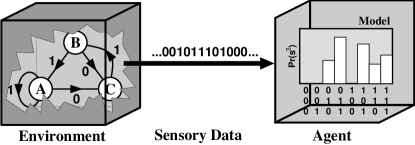
FIG. 1.: The measurement channel: The internal states $\{{\bf A},{\bf B},{\bf C}\}$ of the system are reflected, only indirectly, in the observed measurement of $1$s and $0$s. An observer works with this impoverished data to build a model of the underlying system. After Ref. [1].

One of the central questions addressed in the following is, How does an agent, apprised of the environment’s possible states and behaviors, come to know the state of its environment? We will show that this is related to another question, How does an agent come to accurately estimate how random an environment is? In particular, we investigate how finite-data approximations converge to an asymptotic measure of randomness by introducing several quantities that capture the nature of this convergence. We demonstrate that regularities that are unseen are “converted” to apparent randomness. A more thorough discussion of these results, including proofs of the following propositions and theorems, is found in [2].

II Measurement Channel

We adapt Shannon’s conception of a communication channel as follows: We assume that there is an environment (source or process) that produces a sensory data stream (message)—a string of symbols drawn from a finite alphabet ($\cal A$). The task for the agent (receiver or observer) is to estimate the probability distribution of sequences and, thereby, estimate how random the environment is. Further, we assume that the agent does not know the environment’s structure; the range of its states and their transition structure—the environment’s internal dynamics—are hidden from the agent. (We will, however, relax this assumption in Sec. V below.) Since the agent does not have direct access to the environment’s internal, hidden states, we picture instead that the agent simply collects blocks of measurements from the data stream and stores the block probabilities in a histogram (the internal model). In this scheme, the agent can estimate, to arbitrary accuracy, the probability of measurement sequences by observing for arbitrary lengths of time.

This measurement channel scenario is illustrated in Fig. 1. In this case, the environment is a three-state deterministic finite automaton. However, the agent does not see the internal states $\{{\bf A},{\bf B},{\bf C}\}$. Instead, it has access only to the measurement symbols $\{0,1\}$ generated on state-to-state transitions by the hidden automaton. In this sense, the measurement channel acts like a communication channel; the channel maps from an internal-state sequence $\ldots{\bf BCBAACBC}\ldots$ to a measurement sequence $\ldots 0111010\ldots$. The environment depicted in Fig. 1 belongs to the class of stochastic process known as hidden Markov models. The transitions from internal state to internal state are Markovian, in that the probability of a given transition depends only upon which state the process is currently in. However, these internal states are not seen by the agent—hence the name hidden Markov model [3, 4].

III Entropies: Measuring Randomness

Let ${\rm Pr}(s^{L})$ denote the probability distribution over blocks $s^{L}=s_{0},s_{1},\ldots,s_{L-1}$ of $L$ consecutive environment observations, $s_{i}\in{\cal A}$. Then the total Shannon entropy of these $L$ consecutive measurements is defined to be:

$$H(L)\,\equiv\,-\sum_{s^{L}\in{\cal A}^{L}}{\rm Pr}(s^{L}){\rm log}_{2}{\rm Pr}(s^{L})\;,$$ (1)

where $L>0$. The sum is understood to run over all possible blocks of $L$ consecutive symbols. The units of $H(L)$ are bits. The entropy $H(L)$ measures the uncertainty associated with sequences of length $L$. (For a more detailed discussion of the Shannon entropy and related information theoretic quantities, see, e.g., Ref. [5].) Below, we will focus on the behavior of the Shannon entropy curve $H(L)$. We shall see that examining how $H(L)$ grows with $L$ leads to several quantities that capture aspects of the environment’s randomness and structure.

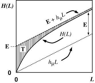
FIG. 2.: Total Shannon entropy growth for a finitary information source: a schematic plot of $H(L)$ versus $L$. $H(L)$ increases monotonically and asymptotes to the line ${\bf E}+h_{\mu}L$, where ${\bf E}$ is the excess entropy and $h_{\mu}$ is the source entropy rate. The shaded area is the transient information ${\bf T}$. For more discussion, see text.

The source entropy rate $h_{\mu}$ is the rate of increase with respect to $L$ of the total Shannon entropy in the large-$L$ limit:

$$h_{\mu}\equiv\lim_{L\rightarrow\infty}\frac{H(L)}{L}\;,$$ (2)

where $\mu$ denotes the measure over infinite sequences that induces the $L$-block joint distribution ${\rm Pr}(s^{L})$; the units are bits/symbol. Alternatively, one can define a finite-$L$ approximation to $h_{\mu}$,

$$h_{\mu}(L)\,=\,H(L)-H(L\!-\!1)\;,$$ (3)

and show [5] that $h_{\mu}=\lim_{L\rightarrow\infty}h_{\mu}(L)$. The entropy rate $h_{\mu}$ quantifies the irreducible randomness in observation sequences produced by the environment—the randomness that persists even after statistics over longer and longer blocks of observations are accounted for by the agent.

IV Excess Entropy: Measuring Memory

Having looked at length-$L$ sequences, an agent can estimate the true randomness $h_{\mu}$ by calculating $h_{\mu}(L)$, defined in Eq. (3). With enough sensory data it can get good approximations to $h_{\mu}$ by using long sequences. But what if there is insufficient data to allow this? To answer this we must determine how the estimates $h_{\mu}(L)$ converge to $h_{\mu}$? One measure of convergence is provided by the excess entropy ${\bf E}$:

$${\bf E}\,\equiv\,\sum_{L=1}^{\infty}[h_{\mu}(L)-h_{\mu}]\;,$$ (4)

The units of ${\bf E}$ are bits. The excess entropy is not a new quantity; it was first introduced almost two decades ago [6, 7]. For recent reviews see [2, 8, 9].

${\bf E}$ measures the convergence of $h_{\mu}(L)$ and plays a role in determining how an agent comes to know how random its environment is. But what exactly does ${\bf E}$ measure? The length-$L$ approximation $h_{\mu}(L)$ overestimates the entropy rate $h_{\mu}$ at finite $L$ by an amount $h_{\mu}(L)-h_{\mu}$. This difference measures how much more random single measurements appear using the finite $L$-block statistics than the statistics of infinite sequences. In other words, this excess randomness tells us how much additional information must be gained from the environment in order to reveal the actual per-symbol uncertainty $h_{\mu}$. Thus, we can think of the difference $h_{\mu}(L)-h_{\mu}$ as the redundancy (per symbol) in length-$L$ sequences: that portion of information-carrying capacity in the $L$-blocks which is not actually random, but is due instead to correlations. The excess entropy ${\bf E}$, then, is the total amount of this redundancy and, as such, a measure of one type of memory intrinsic to an environment.

The next proposition establishes a geometric interpretation of ${\bf E}$ and an asymptotic form for $H(L)$.

Proposition 1

The excess entropy is the subextensive part of $H(L)$; that is,

$${\bf E}=\lim_{L\rightarrow\infty}[H(L)-h_{\mu}L]\;.$$ (5)

This proposition implies the following asymptotic form for $H(L)$:

$$H(L)\,\sim\,{\bf E}+h_{\mu}L\,,\;{\rm as}\;L\rightarrow\infty\;.$$ (6)

Thus, we see that ${\bf E}$ is the $L=0$ intercept of the linear function Eq. (6) to which $H(L)$ asymptotes. This observation, also made in Refs. [7, 9, 10, 11], is shown graphically in Fig. 2.

Another way to understand excess entropy is through its expression as a type of mutual information.

Proposition 2

The excess entropy is the mutual information between the past and the future:

$${\bf E}\,=\,\lim_{L\rightarrow\infty}I[s_{0}s_{1}\cdots s_{2L-1};s_{2L}s_{2L+1}s_{2L-1}]\;,$$ (7)

when the limit exists.

Eq. (7) says that ${\bf E}$ measures the amount of historical information stored in the present that is communicated to the future. For a discussion of some of the subtleties associated with this interpretation, however, see Ref. [8]. Prop. 2 also shows that ${\bf E}$ can be interpreted as the cost of amnesia: If an agent suddenly loses track of its environment, so that it cannot be predicted at an error level determined by the entropy rate $h_{\mu}$, then the environment appears more random by a total of ${\bf E}$ bits.

V Transient Information: A Measure of Synchronization

We now introduce a quantity that answers the question, How does $H(L)$ converge to its asymptote ${\bf E}+h_{\mu}L$? That is, when has an agent made a sufficient number of observations that it can determine the complexity of its environment? The answer to these questions is provided by the transient information ${\bf T}$:

$${\bf T}\equiv\sum_{L=0}^{\infty}\left[{\bf E}+h_{\mu}L-H(L)\right]\;.$$ (8)

Note that the units of ${\bf T}$ are bits $\times$ symbols. The transient information is a new quantity, recently introduced by us in Ref. [2].

Thus, for finite-memory (${\bf E}$ and ${\bf T}$ finite) processes $H(L)$ scales as ${\bf E}+h_{\mu}L$ for large $L$. When this scaling form is attained, we say that the agent is synchronized to the environment. In other words, when

$${\bf T}(L)\,\equiv\,{\bf E}+h_{\mu}L-H(L)\,=\,0\;,$$ (9)

we say the agent is synchronized at length-$L$ sequences. As we will see below, agent-environment synchronization corresponds to the agent being in a condition of knowledge such that it can predict the environmental observations at an error rate commensurate with to the environment’s entropy rate $h_{\mu}$. We refer to ${\bf T}$ as transient since during synchronization the agent’s prediction probabilities change, stabilizing only after it has collected a sufficient number of observations.

To ground this interpretation, we can establish a direct relation between the transient information ${\bf T}$ and the amount of information required for synchronization to block-Markovian environments. Assume that the agent has a correct model ${\cal M}=\{{\cal V},T\}$ of the environment, where ${\cal V}$ is a set of states and $T$ is the rule governing transitions between states. The task for the agent is to make observations and determine the state $v\in{\cal V}$ of the environment. Once the agent knows with certainty the current state, it is synchronized to the environment, and the average per-symbol uncertainty is exactly $h_{\mu}$. We are interested in describing how difficult it is to synchronize to a directly observed Markov process.

The agent’s knowledge of ${\cal V}$ is given by a distribution over the states $v\in{\cal V}$. Let ${\rm Pr}(v|s^{L},{\cal M})$ denote the distribution over $\cal V$, given that the particular sequence $s^{L}$ has been observed and the agent has internal model ${\cal M}$. The entropy of this distribution measures the agent’s average uncertainty in predicting $v\in{\cal V}$. Averaging this uncertainty over the possible length-$L$ sequences, we obtain the average agent-environment uncertainty:

$${\cal H}(L)\,\equiv$$ (11)

$$\,-\sum_{s^{L}}{\rm Pr}(s^{L})\sum_{v\in{\cal V}}{\rm Pr}(v|s^{L},{\cal M})\log_{2}{\rm Pr}(v|s^{L},{\cal M})\;.$$

The quantity ${\cal H}(L)$ can be used as a criterion for synchronization. The agent is synchronized to the environment when ${\cal H}(L)=0$—that is, when the agent is completely certain about the state $v\in\cal V$ of the mechanism generating the sequence. When the condition in Eq. (9) is met, we see that ${\cal H}(L)=0$, and the uncertainty associated with the prediction of the model ${\cal M}$ is exactly $h_{\mu}$.

However, while the agent is still unsynchronized ${\cal H}(L)>0$. We refer to the total average uncertainty experienced by an agent during the synchronization process as the synchronization information ${\bf S}$:

$${\bf S}\equiv\sum_{L=0}^{\infty}{\cal H}(L)~{}.$$ (12)

The synchronization information measures the average total information that must be extracted from observations so that the agent is synchronized.

In the following, we assume that the environment is Markovian of order $R$. In contrast to the scenario depicted in Fig. 1, we assume that the Markov model is not hidden, in the sense that internal states are directly observable.

Theorem 1

For an order-$R$ Markovian environment, the synchronization information ${\bf S}$ is given by:

$${\bf S}={\bf T}+\frac{1}{2}R(R+1)h_{\mu}\;.$$ (13)

Thus, the transient information ${\bf T}$—together with the entropy rate $h_{\mu}$ and the order $R$ of the Markov process—measures how difficult it is to synchronize to an environment. If a system has a large ${\bf T}$, then, on average, an agent will be highly uncertain about the internal state of the environment while synchronizing to it. Thus, ${\bf T}$ measures a structural feature of the environment: how difficult it is for an agent to synchronize to it.

VI Applications and Implications

Using $h_{\mu}$, ${\bf E}$, and ${\bf T}$ one can distinguish various types of entropy convergence and different structural classes of environment. We can now return to the set of questions posed in the introduction: How can we untangle different sources of apparent randomness? In particular, what happens to estimates of the environment’s randomness if we ignore its structure?

Here we show that there are direct and empirically important consequences for ignoring structural properties. Namely, missed regularities are converted to apparent randomness, assumed memory produces false predictability, and assumed synchronization leads to memory underestimates. These result in a range of misleading inferences about both the environment’s randomness and its structure. We consider four different issues:

1. What happens when an agent ignores entropy-rate convergence?

2. What happens when the environment’s apparent memory is ignored?

3. What happens if the agent ignores synchronization?

4. What happens if the agent assumes it is synchronized to the environment, when it is not?

A Disorder as the Price of Ignorance

The first two questions are closely related and rather straightforward to answer. The preceding sections defined several different quantities—$h_{\mu}$, ${\bf E}$, and ${\bf T}$—that measure randomness, memory, synchronization, and other features of a process. For the most part, these are asymptotic quantities in the sense that they involve the behavior of the function $H(L)$ in the $L\rightarrow\infty$ limit. Thus, their exact empirical estimation demands that an infinite number of measurements (for accurate estimates of sequence probabilities) of infinitely long sequences be made. Obviously, other than by analytic means, it is not possible to calculate exactly such quantities. Exact, $L\rightarrow\infty$ results are known for only a few special processes that are analytically tractable.

This leads one to ask, Even when sequence probabilities are accurately known, how well can these various environment properties be estimated at finite $L$? What errors are introduced, and are these errors related in any way?

The simplest such question, the first one listed above, arises when one attempts to estimate source randomness $h_{\mu}$ via the approximation $h_{\mu}(L)$. Generally, stopping the estimate at finite $L$ gives one a rate $h_{\mu}(L)$ which is larger than the actual rate $h_{\mu}$. That is, the environment appears more random if we ignore correlations between observations separated by more than $L$ steps. For a discussion of several methods to improve on the estimator $h_{\mu}(L)$ in the context of dynamical systems, see Ref. [12].

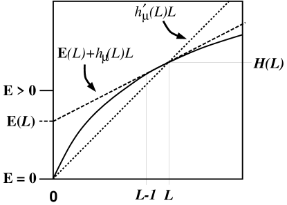
FIG. 3.: Ignored memory is converted to randomness: Illustration of how ignoring memory, in this case implicitly assuming ${\bf E}=0$ as Eq. (2) implies, when actually ${\bf E}>0$, leads to an overestimate $h_{\mu}^{\prime}(L)$ (slope of dotted line) of the actual entropy rate $h_{\mu}$ (slope of dashed line).

An agent could also estimate $h_{\mu}$ at finite $L$ by using $h_{\mu}^{\prime}(L)=H(L)/L$, as suggested by Eq. (2). Using this definition to estimate $h_{\mu}$ is tantamount to assuming that ${\bf E}=0$, as illustrated by the dashed line $h_{\mu}^{\prime}L$ in Fig. 2. Now suppose an agent makes measurements of an environment with entropy rate $h_{\mu}$ and excess entropy ${\bf E}>0$. Then, at a given $L$, we can ask what the entropy rate estimate $h_{\mu}^{\prime}(L)=H(L)/L$ is. As shown in [2], $h_{\mu}^{\prime}(L)\geq h_{\mu}(L)\geq h_{\mu}$. But how much more random does the environment appear? This is answered in a straightforward way by the following proposition.

Proposition 3

When the agent is synchronized to the environment,

$$h_{\mu}^{\prime}(L)-h_{\mu}=\frac{{\bf E}}{L}~{}.$$ (14)

In this way, ${\bf E}$ bits of memory are converted into additional, apparent randomness. The environment appears more random due to the agent’s ignoring one of its structural properties.

Although ${\bf E}$ is an $L$-asymptotic quantity, the error ${\bf E}/L$ in the entropy-rate estimate dominates at small $L$. Moreover, being restricted to small $L$ is typical of experimental situations with limited data or in which drift is present. One cannot reliably estimate the $L$-block probabilities ${\rm Pr}(s^{L})$ at large $L$ due to the exponential growth in their number or the nonstationarity of block probabilities, respectively.

B Predictability and Instantaneous Synchronization

Conversely, if one assumes a fixed amount of memory ${\bf E}$, we shall see that this leads to an underestimate of the entropy rate $h_{\mu}$ and the environment appears more predictable than it is. Assuming a fixed excess entropy is not something that one is likely to do in the particular setting here, in which an agent empirically measures entropy density and related quantities from observation sequences. In a more general modeling setting, however, one always runs the risk of using too large a model and, in so doing, “projecting” some particular structure—such as, additional memory capacity—onto the environment. Assuming a fixed, nonzero value for the excess entropy is, in an abstract sense, an example of over-fitting. Given this, we ask, What is the consequence of assuming a fixed value for ${\bf E}$?

Equivalently, what happens if the agent assumes that it is synchronized to the environment at some finite $L$, implying that $H(L)={\bf E}+h_{\mu}L$ at that $L$? The geometric construction for this scenario is given in Fig. 4. In effect the environment is erroneously considered to be a completely observable Markovian process in which $H(L)$ converges to its asymptotic form exactly at some finite $L$ [2, 13]. If the agent then uses its assumed value for ${\bf E}$, one arrives at the estimator $\widehat{h_{\mu}}$ where

$$\widehat{h_{\mu}}\,\equiv\,\frac{H(L)-{\bf E}}{L}\,\neq h_{\mu}\;.$$ (15)

At a given $L$ the effect is that the agent considers the environment to have a larger ${\bf E}$ than it actually has at that $L$. The line ${\bf E}+\widehat{h_{\mu}}L$ appears fixed at ${\bf E}$ when that intercept should be lower at the given $L$. The result, easily gleaned from Fig. 4, is that the entropy rate $h_{\mu}$ is underestimated as $\widehat{h_{\mu}}$. (The two entropy rates are the slopes of the two straight lines.) In other words, the agent will believe the environment to be more predictable than it actually is.

Proposition 4

  An agent monitors an environment with excess entropy ${\bf E}>0$. If the agent assumes it is synchronized when it is not, then

$$\widehat{h_{\mu}}\leq h_{\mu}\;.$$ (16)

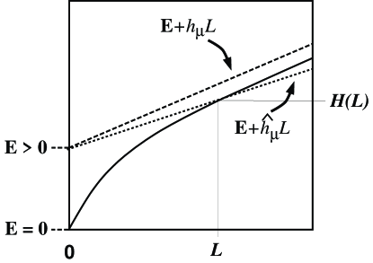
FIG. 4.: Assumed synchronization converted to false predictability: Schematic illustration of how assuming one is synchronized, leads to an underestimate $\widehat{h_{\mu}}$ (slope of dotted line) for an environment with excess entropy ${\bf E}>0$ and entropy rate $h_{\mu}$ (slope of dashed line).

C Assumed Synchronization Implies Reduced Apparent Memory

In addition to analyzing the effects on the apparent entropy rate due to assuming synchronization, we can ask a complementary question: What are the effects of assuming synchronization on estimates $\widehat{{\bf E}}$ of the apparent memory? Figure 5 illustrates this situation.

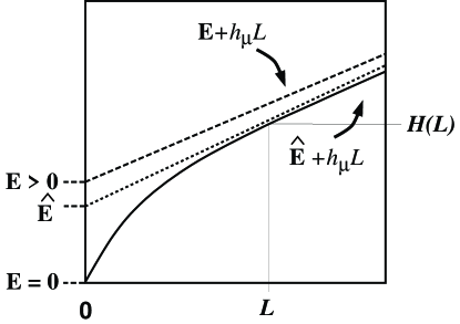
FIG. 5.: Assumed synchronization leads to less apparent memory: Schematic illustration of how assuming synchronization to an environment, in this case implicitly assuming $H(L)={\bf E}+h_{\mu}L$, leads to an underestimate $\widehat{{\bf E}}$ of the actual memory ${\bf E}>0$.

If, at a given $L$, we approximate the entropy rate estimate $h_{\mu}(L)=H(L)-H(L-1)$ by the true entropy $h_{\mu}$, then the offset between the asymptote and $H(L)$ is simply ${\bf E}+h_{\mu}L-H(L)$. Thus, looking at Fig. 5, we see that we have a reduced apparent memory $\widehat{{\bf E}}\leq{\bf E}$ of

$$\widehat{{\bf E}}=H(L)-h_{\mu}L~{}.$$ (17)

In fact, since the estimated entropy rate is larger than $h_{\mu}$, the reduction in apparent memory is even larger. Thus, assuming synchronization, in the sense that $h_{\mu}(L)=h_{\mu}$, leads one to underestimate the apparent memory, as measured by the excess entropy ${\bf E}$. And so, the environment appears less structurally complex than it is.

VII Conclusion

We have reviewed several information theoretic measures of an environment’s randomness and several of its structural properties. We also introduced a new quantity, the transient information ${\bf T}$. One of the central results of this work is contained in Theorem 1, which states that ${\bf T}$ is directly related to the total agent-environment uncertainty experienced while an agent synchronizes to a Markovian environment.

We then considered various trade-offs between finite-$L$ estimates of the excess entropy ${\bf E}$ and the entropy rate $h_{\mu}$. In particular, we showed that if an agent does not take one or another into account it will systematically over- or underestimate an environment’s entropy rate $h_{\mu}$. For example, there can be an inadvertent conversion of ignored memory into apparent randomness. The magnitude oa f this effect is proportional to the difference between environment memory and the upper bound on memory that the agent store in its internal model. In a complementary way, one can inadvertently convert assumed memory into false predictability. As a result, an agent must have some method for accounting for an environment’s structural features, even if it’s focus is only on the apparently simple question of how random a process is [14].

REFERENCES

- [1] J. P. Crutchfield. Semantics and thermodynamics. In M. Casdagli and S. Eubank, editors, Nonlinear Modeling and Forecasting, volume XII of Santa Fe Institute Studies in the Sciences of Complexity, pages 317–359, Reading, Massachusetts, 1992. Addison-Wesley.
- [2] J. P. Crutchfield and D. P. Feldman. Regularities unseen, randomness observed: Levels of entropy convergence. Technical Report Working Paper 01-02-012, arXiv.org/abs/cond-mat/0102181, Santa Fe Institute, 2001.
- [3] D. Blackwell and L. Koopmans. On the identifiability problem for functions of Markov chains. Ann. Math. Statist., 28:1011–1015, 1957.
- [4] R. J. Elliot. Hidden Markov Models: Estimation and Control. Springer-Verlag, 1995.
- [5] T. M. Cover and J. A. Thomas. Elements of Information Theory. John Wiley & Sons, Inc., 1991.
- [6] J. P. Crutchfield and N. H. Packard. Symbolic dynamics of noisy chaos. Physica D, 7:201–223, 1983.
- [7] P. Grassberger. Toward a quantitative theory of self-generated complexity. Intl. J. Theo. Phys., 25(9):907–938, 1986.
- [8] C. R. Shalizi and J. P. Crutchfield. Computational mechanics: Pattern and prediction, structure and simplicity. J. Stat. Phys., 2001. in press.
- [9] W. Bialek, I. Nemenman, and N. Tishby. Predictability, complexity, and learning. physics/0007070v2, 2000.
- [10] R. Shaw. The Dripping Faucet as a Model Chaotic System. Aerial Press, Santa Cruz, California, 1984.
- [11] W. Li. On the relationship between complexity and entropy for Markov chains and regular languages. Complex Systems, 5(4):381–399, 1991.
- [12] T. Schürmann and P. Grassberger. Entropy estimation of symbol sequences. Chaos, 6:414–427, 1996.
- [13] W. Ebeling. Prediction and entropy of nonlinear dynamical systems and symbolic sequences with LRO. Physica D, 109:42–52, 1997.
- [14] J. Ford. How random is a coin toss? Physics Today, pages 40–47, April 1983.