Universality of Velocity Gradients in Forced Burgers Turbulence

Abstract

It is demonstrated that Burgers turbulence subject to large-scale white-noise-in-time random forcing has a universal power-law tail with exponent -7/2 in the probability density function of negative velocity gradients, as predicted by E, Khanin, Mazel and Sinai (1997, Phys. Rev. Lett. 78, 1904). A particle and shock tracking numerical method gives about five decades of scaling. Using a Lagrangian approach, the -7/2 law is related to the shape of the unstable manifold associated to the global minimizer.

The universality of small-scale properties in fully developed Navier–Stokes (NS) turbulence is frequently investigated assuming that a steady state is maintained by a large-scale random force. For structure functions (moments of increments) universality with respect to the force is conjectured in the case of three-dimensional NS turbulence and proven for certain linear passive scalar models (see, e.g., Ref. rmp ). The universality of probability density functions (p.d.f.) for velocity increments and gradients is a difficult question which, so far, has been mostly addressed within the framework of the pressureless model of Burgers turbulence, usually the one-dimensional Burgers equation

$$\partial_{t}u+u\partial_{x}u=\nu\partial_{xx}u+f(x,t)$$ (1)

with white-noise-in-time forcing cy95 . It is generally conjectured that, when $\nu\to 0$ and the forcing is confined to large scales, the tail of the p.d.f. of velocity gradients $\xi$ at large negative values follows a universal power-law $p(\xi)\propto|\xi|^{-\alpha}$. The actual value of the exponent is however a matter of controversy. Let us briefly recall some of the arguments found in the literature.

A standard approach is based on studying the inviscid limit of the Fokker–Planck equation for the p.d.f.

$$\partial_{t}p-\partial_{\xi}\left(\xi^{2}p\right)-\xi p+\nu\partial_{\xi}\left(\left\langle\partial_{xx}\xi|\xi\right\rangle p\right)=B\partial_{\xi\xi}p,$$ (2)

where the right-hand side expresses the diffusion of probability due to the delta-correlation in time of the forcing. It was pointed out by Polyakov p95 that the inviscid limit of (2) contains anomalies due to the singular behavior of the dissipative term $\nu\partial_{\xi}\left(\left\langle\partial_{xx}\xi|\xi\right\rangle p\right)$. The value $\alpha=3$ is obtained if anomalies are ignored gk98 or if a piecewise linear approximation is made for the solutions of the Burgers equation bm96 . An operator product expansion (OPE) method borrowed from quantum field theory has been proposed for evaluating such anomalies and an argument presented in favor of $\alpha=5/2$ (actually, for velocity increments and infinite systems) p95 . However, this expansion leads to a relation involving unknown coefficients which must be determined, e.g., from numerical simulations yc96b98 , and restricts the possible values to $5/2\leq\alpha\leq 3$ b01 . Anomalies cannot be understood without a complete description of the singularities of the solutions, such as shocks, and of their statistical properties. For the case of a space-periodic system (as we shall assume), a crucial observation made in Ref. ekms97 is that large negative gradients stem mainly from preshocks, that is the cubic-root singularities in the velocity preceding the formation of shocks ff83 . A simple argument was given in Ref. ekms97 for determining the fraction of space-time where the velocity gradient is less than some large negative value. This leads to $\alpha=7/2$ provided preshocks do not cluster. Determinations of the dissipative anomaly of (2) have been made by formal matched asymptotics eve99 and by bounded variation calculus eve00 . With the assumption that shocks are born with vanishing amplitude from isolated preshocks, the value $\alpha=7/2$ was obtained eve99 ; eve00 . Other attempts to derive $\alpha=7/2$ using also isolated preshocks have been made sevenhalf . Note that there are simpler instances, including time-periodic forcing bfk00 and decaying Burgers turbulence with smooth random initial conditions eve00 ; bf00 , which fall in the universality class $\alpha=7/2$, as can be shown by systematic asymptotic expansions using a Lagrangian approach. In the presence of forcing, the key issues which remained to be settled are the possible clustering of preshocks and, closely related to this, the possible birth of shocks with non-vanishing amplitude. The results presented hereafter almost completely rule out such possibilities.

Numerically solving the randomly forced Burgers equation in the limit of vanishing viscosity in such a way as to obtain clean scaling for the p.d.f. of gradients represents a significant challenge. Broadly speaking, there are two classes of methods. On the one hand, methods involving a small viscosity, either introduced explicitly (e.g. in a spectral calculation) or stemming from discretization (e.g. in a finite difference calculation). Viscosity gives rise to a power-law range with exponent $-1$ at very large negative gradients gk98 whose presence will make the inviscid $|\xi|^{-\alpha}$ range appear shallower than it actually is, unless extremely high spatial resolution is used. On the other hand, there are methods which directly capture the inviscid limit with the appropriate shock conditions such as the fast Legendre transform method of Ref. nv94 (extended to the forced case in Ref. bfk00 ). This method is very well adapted to decaying Burgers turbulence with non-smooth Brownian-type initial data vdun94 but, with spatially smooth forcing, it leads to delicate interpolation problems which have been overcome in the case of time-periodic forcing bfk00 ; with white-noise-in-time forcing, it is difficult to prevent spurious accumulations of preshocks leading to $\alpha=3$. To avoid such pitfalls, we develop a Lagrangian particle and shock tracking method notebennaim which is able to cleanly separate smooth parts of the solution and is particularly effective for identifying preshocks. The main idea of the method is to consider the evolution of a set of $N$ massless point particles accelerated by a discrete-in-time approximation of the forcing with a uniform time step. When two of these particles intersect, they merge and create a new type of particle, a shock, characterized by its velocity (half sum of the right and left velocities of merging particles) and its amplitude. The particle-like shocks then evolve as ordinary particles, capture further intersecting particles and may merge with other shocks. In order not to run out of particles too quickly, the initial small region where particles have the least chance of being subsequently captured is determined by localization of the global minimizer (see below). The calculation is then restarted from $t=0$ for the same realization of forcing but with a vastly increased number of particles in that region. This method gives complete control over shocks and preshocks notefilm and allows an accurate determination of the relevant statistical quantity while keeping a manageable number of degrees of freedom.

Fig. 1 shows the p.d.f. of the velocity gradients in log-log coordinates at negative values for a Gaussian forcing restricted to the first three Fourier modes with equal variances such that the large-scale turnover time is order unity. Quantitative information about the value of the exponent is obtained by measuring the “local scaling exponent”, i.e. the logarithmic derivative of the p.d.f. calculated here using least-square fits on half-decades. It is seen that over about five decades, the local exponent is within less than 1% of the value $-7/2$ predicted by E et al. ekms97 . This value of the exponent was also obtained numerically (with a fewer particles) for other large-scale forcing instances with compactly supported or exponentially decreasing spectra and also for non-Gaussian forcing (e.g. with Fourier amplitudes having a Bernoulli distribution or an uniform distribution in an interval). Evidence for non-clustering of preshocks is obtained by counting the average number of shock formations per unit time. For different types of large-scale forcing, we found that the typical mean number of preshocks per turnover time is comparable to the number of forcing Fourier modes significantly excited. For such forcings, the density of preshocks is found to vary by not more than 6% when the time step varies by two orders of magnitude around $\delta t=10^{-4}$, which is hardly consistent with a power-law (and even a logarithmic) divergence as $\delta t\to 0$. Furthermore, we have checked that shocks are always born with vanishing amplitude (within numerical errors).

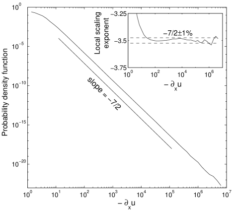
Figure 1: P.d.f. of the velocity gradient at negative values in log-log coordinates obtained by averaging over 20 realizations and a time interval of 5 units of time (after relaxation of transients). The simulation involves up to $N=10^{5}$ particles and the forcing is applied at discrete times separated by $\delta t=10^{-4}$. Upper inset: local scaling exponent.

Turning now to theoretical results, let us briefly recall the construction of solutions developed by E et al. ekms00 , in terms of the dynamical system associated to the characteristics of (1) in the inviscid limit note . The force is assumed to derive from a Gaussian potential $F(x,t)$, delta-correlated in time, periodic of period 1 and analytic in space. A statistically stationary régime is reached by taking the initial time at $-\infty$. The central point of the construction is the following variational characterization of the solution at an arbitrary time ($t=0$ chosen for convenience):

$$u(x,0)={\partial\over\partial x}\min_{X(\cdot)}\left[\int_{-\infty}^{0}\left[{1\over 2}\dot{X}^{2}(t)-F\left(X(t),t\right)\right]dt\right],$$ (3)

where the minimum is taken over all piecewise smooth (absolutely continuous) curves $X(t)$ with $t\in(-\infty,0]$ such that $X(0)=x$. A curve minimizing the action in (3) is called a minimizer and should be understood as a fluid particle trajectory. It obviously has to satisfy for all $t<0$ the Euler–Lagrange equations:

$$\dot{X}(t) = U(t),$$ (4)

$$\dot{U}(t) = f(X(t),t).$$ (5)

Except for a finite number of $x$-values, there exists a unique minimizer ekms00 . The locations where there are more than one minimizer correspond to shocks. The minimizers converge exponentially fast backward in time to the trajectory of the unique fluid particle which is never absorbed by a shock. This trajectory is called the global minimizer because its action is minimal at any time; it corresponds to a hyperbolic trajectory of the dynamical system (4)-(5). Associated to it, there are two curves in the phase-space $(x,u)$: a stable (attracting) manifold $\Gamma^{\rm(s)}$ and an unstable (repulsive) manifold $\Gamma^{\rm(u)}$. The minimizers converge backward in time to the global minimizer and, thus, the graph of the solution is made of pieces of the unstable manifold with jumps at shocks. One of these shocks, called the main shock, is singled out. It is the unique shock which has always existed in the past (whereas generic shocks are born at some finite time $t<0$); it may be shown that it corresponds to the position giving rise to the left-most and the right-most minimizers which approach the global one backward in time. The other shocks cut through the doublefold loops of the unstable manifold (see Fig. 2). We observe that their locations can be obtained by a Maxwell rule applied to those loops. Indeed, the difference of the two areas defined by cutting such a loop at some position $x$ is equal to the difference of actions of the two minimizers defined by the upper and lower branches and, thus, vanishes at the shock location.

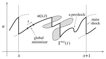
Figure 2: Sketch of the unstable manifold $\Gamma^{\rm(u)}$ in the $(x,u)$ plane at a time $t$ with a preshock occurring. Shock locations are obtained by applying Maxwell rules to the loops. The velocity is shown as a bold line.

We also observe that the structure just outlined has much in common with that appearing in the unforced Burgers equation. Indeed when $f=0$, the solution to the Burgers equation can be constructed from the Lagrangian manifold in the $(x,u)$ plane, defined as the position and the velocity of fluid particles when ignoring shocks. This manifold is parameterized by the Lagrangian coordinate $a$; denoting $u_{0}$ the initial velocity, we then have simply $x=a+tu_{0}(a)$ and $u=u_{0}(a)$. The actual solution with shocks is obtained by applying the standard Maxwell rule to the Lagrangian manifold. In the forced case, a parameterization of the unstable manifold (e.g. by the arclength) is now the analog of the Lagrangian coordinate. But there are two important differences: first, in the unforced case, the time evolution of the Lagrangian manifold is explicit and linear while, in the presence of a force, the Euler–Lagrange equations (4)-(5) are not, in general, explicitly solvable and the unstable manifold has a hyperbolic dynamic. Second, the smoothness of the Lagrangian manifold in the unforced case stems directly from the smoothness of the initial data, whereas in the forced case Pesin’s theory must be used to show that when the force is indefinitely differentiable in space, so is the unstable manifold ekms00 .

Using the smoothness of the unstable manifold, we now formally derive the $-7/2$ law, by an argument mostly borrowed from the unforced case bf00 . Let $\Gamma^{\rm(u)}=\{(X(s),U(s))\}$ with $s$ real, be a parameterization of the unstable manifold at time $t=0$. It is assumed for convenience that $s=0$ corresponds to the global minimizer and that $X^{\prime}(0)>0$, where primes denote $s$-derivatives. The velocity is exactly obtained by eliminating from the unstable manifold the shaded areas determined by the Maxwell rules and the parts beyond the main shock (shown as dashed lines in Fig. 2). The surviving set of parameter values (excluding shocks) is denoted $\Omega$. Turning to the statistical description, the p.d.f. of velocity gradients may be written

$$p(\xi)=\left\langle\delta\left(\partial_{x}u(x,0)-\xi\right)\right\rangle.$$ (6)

Because of homogeneity, we can integrate over the space period and then change from the $x$ variable to the $s$ variable to obtain

$$p(\xi)=\int_{0}^{1}p(\xi)dx=\left\langle\int_{\Omega}\delta\left({U^{\prime}\over X^{\prime}}-\xi\right)X^{\prime}ds\right\rangle.$$ (7)

Note that since a finite gradient is assumed, $x$ cannot be at a shock position. Denoting by $s_{k}$ the parameter values where the argument of the delta function vanishes, we obtain

$$p(\xi)=\left\langle\sum_{k}{X^{\prime 2}\over|U^{\prime\prime}-\xi X^{\prime\prime}|}\delta(s-s_{k})ds\right\rangle.$$ (8)

For very large negative values of $\xi$, the $s_{k}$’s must be near some $s_{*j}$, corresponding to a local minimum of $X^{\prime}$. Taylor expansions of $X$ and $U$ in the vicinities of the $s_{*j}$’s and the use of the Maxwell rule show that the $s_{*j}$’s are located in space-time near preshocks satisfying $X^{\prime}=0$ and $X^{\prime\prime}=0$ with $X^{\prime\prime\prime}>0$ (see Fig. 2). Proceeding as in Ref. bf00 , we finally obtain, to leading order

$$p(\xi)\simeq C|\xi|^{-7/2},\qquad\xi\to-\infty,$$ (9)

$$C={5\sqrt{2}\over 2}\left\langle\int_{\Omega,X^{\prime\prime\prime}>0}|X^{\prime\prime\prime}|^{1/2}|U^{\prime}|^{5/2}\delta(X^{\prime})\delta(X^{\prime\prime})ds\right\rangle.$$ (10)

Hence, the constant involves the mean of $|X^{\prime\prime\prime}|^{1/2}|U^{\prime}|^{5/2}$ at preshocks. Its evaluation requires the knowledge of the joint probability distribution of $X^{\prime}$, $X^{\prime\prime}$, $X^{\prime\prime\prime}$ and $U^{\prime}$. From the Euler–Lagrange equations (4)-(5), we observe that a set of ordinary differential equations with nonlinear stochastic forcing is easily obtained for $X$, $U$ and the aforementioned four variables. From these equations, using techniques similar to those developed in Ref. ekms00 (where a subset of these stochastic equations is studied), it should be possible, on the one hand, to make our derivation more rigorous (including for the non-clustering of preshocks) and, on the other hand, to obtain an upper bound for the constant $C$ in the $-7/2$ law. Note that the expression for $C$ involves also an integral over the admissible set of parameters $\Omega$ whose determination cannot in general be done by local analysis with ordinary differential equations. This is why only an upper bound is expected.

As noted in Ref. ekms97 , the universality with respect to the forcing of the p.d.f. of large negative velocity gradients may be extended to negative velocity increments, provided that they are not significantly influenced by shocks. Without understanding of all the mechanisms leading to small-amplitude shocks in the forced case, the issue of universality for the p.d.f.’s of velocity increments cannot be settled. A first step would be to determine numerically the distribution of shock amplitudes. Note that our technique may also be extended to the case of forcing at scales much smaller than the size of the system, a problem close to that considered by Polyakov p95 , which is left for future work.

I wish to express my gratitude to U. Frisch and K. Khanin for numerous helpful discussions and encouragements. I also thank M. Blank, G. Eyink, A. Fouxon, R. Mohayaee, E. Vanden Eijnden, M. Vergassola and V. Yakhot for useful remarks. Work in Nice was supported by the European Union, under contract HPRN-CT-2000-00162; work at CNLS was supported by the U.S. Department of Energy, under contract W-7405-ENG-36. Simulations were performed on Avalon at the Los Alamos National Laboratory.

References

- (1) G. Falkovich, K. Gawȩdzki and M. Vergassola, Particles and fields in fluid turbulence, submitted to Rev. Mod. Phys. (2001).
- (2) A. Chekhlov and V. Yakhot, Phys. Rev. E 51, R2739 (1995).
- (3) A. Polyakov, Phys. Rev. E 52, 6183 (1995).
- (4) T. Gotoh and R.H. Kraichnan, Phys. Fluids 10, 2859 (1998).
- (5) J.-P. Bouchaud and M. Mézard, Phys. Rev. E 54, 5116 (1996).
- (6) V. Yakhot and A. Chekhlov, Phys. Rev. Lett. 77, 3118 (1996); S. Boldyrev, Phys. Plasmas 5, 1681 (1998).
- (7) S. Boldyrev, personal communication (2001).
- (8) W. E, K. Khanin, A. Mazel and Ya. Sinai, Phys. Rev. Lett. 78, 1904 (1997).
- (9) J.D. Fournier and U. Frisch, J. Méc. Théor. Appl. 2, 699 (1983).
- (10) W. E and E. Vanden Eijnden, Phys. Rev. Lett. 83, 2572 (1999).
- (11) W. E and E. Vanden Eijnden, Comm. Pure Appl. Math. 53, 852 (2000).
- (12) R.H. Kraichnan, Phys. Fluids 11, 3738 (1999); I. Kolokolov and V. Lebedev, nlin.CD/0012037 (2000).
- (13) J. Bec, U. Frisch and K. Khanin, J. Fluid Mech. 416, 239 (2000).
- (14) J. Bec and U. Frisch, Phys. Rev. E 61, 1395 (2000).
- (15) A. Noullez and M. Vergassola, J. Sci. Comput. 9, 259 (1994).
- (16) M. Vergassola, B. Dubrulle, U. Frisch and A. Noullez, Astron. Astrophys. 289, 325 (1994).
- (17) Particle tracking methods are also very effective for studying inelastic gases; see E. Ben-Naim, S.Y. Chen, G.D. Doolen and S. Redner, Phys. Rev. Lett. 83, 4069 (1999).
-
(18)
A movie showing the global evolution over a few turnover times
is available at
http://sclavis.obs-nice.fr/~bec/burgers.html - (19) W. E, K. Khanin, A. Mazel and Ya.G. Sinai, Ann. Math. 151, 877 (2000).
- (20) An elementary introduction to the concepts of minimizers and main shock may be found in Ref. bfk00 for the case of periodic forcing.