Bifurcation Diagram for Compartmentalized Granular Gases

Abstract

The bifurcation diagram for a vibro-fluidized granular gas in $N$ connected compartments is constructed and discussed. At vigorous driving, the uniform distribution (in which the gas is equi-partitioned over the compartments) is stable. But when the driving intensity is decreased this uniform distribution becomes unstable and gives way to a clustered state. For the simplest case, $N=2$, this transition takes place via a pitchfork bifurcation but for all $N>2$ the transition involves saddle-node bifurcations. The associated hysteresis becomes more and more pronounced for growing $N$. In the bifurcation diagram, apart from the uniform and the one-peaked distributions, also a number of multi-peaked solutions occur. These are transient states. Their physical relevance is discussed in the context of a stability analysis.

I Introduction

One of the key features of a granular gas is the tendency to spontaneously separate into dense and dilute regions goldhirsch93 ; mcnamara94 ; du95 ; jaeger96 ; kudrolli97 ; kadanoff99 . This clustering phenomenon manifests itself in a particularly clear manner in a box that is divided in a series of $N$ connected compartments, with a hole (at a certain height) in the wall between each two adjacent compartments. The system is vibro-fluidized by shaking the box vertically. With vigorous shaking the granular material is observed to be distributed uniformly over the compartments as in any ordinary molecular gas. Below a certain driving level however, the particles cluster in a small subset of the compartments, emptying all the others.

For $N=2$ the transition from the uniform to the clustered state is of second order, taking place through a pitchfork bifurcation eggers99 . For $N=3$ it was recently found that the transition is hysteretic. It is a first order phase transition, involving saddle-node bifurcations vdweele00 . This difference has been explained by a flux model. In the present paper we will use the same flux model to construct the bifurcation diagrams for arbitrary $N$.

The main ingredient of this model is a flux function $F(n)$, which gives the outflow from a compartment to one of its neighbors as a function of the fraction of particles ($n$) contained in the compartment eggers99 . The function $F(n)$ starts out from zero at $n=0$ and initially increases with $n$. At large values of $n$ it decreases again because the particles lose energy in the non-elastic collisions, which become more and more frequent with increasing particle density. So $F(n)$ is non-monotonic, and that is why the flux from a well-filled compartment can balance that from a nearly empty compartment.

Assuming that the granular gas in each compartment is in thermal equilibrium at any time (in the sense of the granular temperature mcnamara98 ) the following approximate form for $F(n)$ can be derived eggers99 :

$$F(n_{k})=An_{k}^{2}e^{-BN^{2}n_{k}^{2}},$$ (1)

which is a one-humped function, possessing the features discussed before (See Fig. 1). In the above equation $n_{k}$ is the fraction of particles in the $k$-th compartment, normalized to $\sum n_{k}=1$. The factors $A$ and $B$ depend on the number of particles and their properties (such as the radius, and the restitution coefficient of the interparticle collisions), on the geometry of the system (such as the placement and form of the aperture between the compartments), and on the driving parameters (frequency and amplitude). The factor $A$ determines the absolute rate of the flux, and will be incorporated in the time scale, which thus becomes dimensionless. The clustering transition is governed only by $B$.

The time rate of change $\dot{n}_{k}$ of the particle fraction in the $k$-th compartment is given by the inflow from its two neighbours minus the outflow from the compartment itself,

$$\dot{n}_{k}=F(n_{k-1})-2F(n_{k})+F(n_{k+1}),$$ (2)

with $k=1,2,..,N$. Here we have assumed that the interaction is restricted to neighboring compartments only.

For a cyclic arrangement the above equation is valid for all $N$ compartments (with $k=N+1$ equal to $k=1$). If we take non-cyclic boundary conditions, by obstructing the flux between two of the compartments, the equation has to be modified accordingly for these compartments.

The total number of particles in the system is conserved ($\sum_{k}n_{k}=1$), so

$$\sum_{k}\dot{n}_{k}=0.$$ (3)

Statistical fluctuations in the system would add a noise term to Eq. (2), but we will not consider such a term here. So the present analysis has to be interpreted as a mean field theory for the system.

Equation (2) can also be written in matrix-form, as $\mathbf{\dot{n}}=\mathbf{M}\cdot\mathbf{F}$, or more explicitly:

$$\dot{n}_{k} =\sum_{l}M_{kl}F(n_{l})$$ (4)

$$=\left(\begin{smallmatrix}-2&1&0&0&\cdots&0&1\\ 1&-2&1&0&\cdots&0&0\\ 0&1&-2&1&\cdots&0&0\\ :&:&:&:&&:&:\\ :&:&:&:&&:&:\\ 1&0&0&0&\cdots&1&-2\end{smallmatrix}\right)\cdot\left(\begin{smallmatrix}F(n_{1})\\ F(n_{2})\\ F(n_{3})\\ :\\ :\\ F(n_{N})\end{smallmatrix}\right)$$

Figure 1: The solutions $n_{-}$ and $n_{+}$ of $F(n_{k})=constant$, cf. Eq. 5. Also shown is how the flux balance responds to an increase of $n_{-}$ by an amount of $\delta n$ (see also Eq. 11). The diagram on the right hand side depicts the relation between $F$ and the quantity $\sigma=F^{\prime}(n_{+})/F^{\prime}(n_{-})$, which plays an important role in the stability analysis of section 3.

The given matrix $\mathbf{M}$ corresponds to a cyclic arrangement of the $N$ compartments. A similar matrix can be written down for the case of a non-cyclic arrangement. We will come back to this later, when we will see that most of the results for the cyclic arrangement carry over to the non-cyclic case.

It is easily seen, from the fact that the elements of each row of $\mathbf{M}$ sum up to zero, that $\mathbf{1}=(1,1,\ldots,1)$ is an eigenvector. The corresponding eigenvalue $\lambda=0$ physically reflects the fact that the compartments cannot all be filled (or emptied) simultaneously: $\sum_{k}\dot{n}_{k}=0$ or $\sum_{l}M_{lk}=0$. For future reference we note that all the other eigenvalues of $\mathbf{M}$ are negative (see Appendix).

The remainder of the paper is set up as follows. In Section II we show how to construct the bifurcation diagram, on the basis of Eq. (4), for an arbitrary number of compartments. In Section III we discuss the stability of the various branches in the diagram. Section IV discusses the physical consequences resulting from the diagram, in particular in the limit for $N\to\infty$. Finally, Section V contains concluding remarks. The paper is accompanied by a mathematical Appendix, in which some essential results concerning the stability analysis are derived.

II Constructing the bifurcation diagram

To calculate the bifurcation diagram, we have to find the fixed points of Eq. (4) as a function of the parameter $B$, i.e., those points for which $\dot{n}_{k}=\mathbf{M}\cdot\mathbf{F}=0$. So $\mathbf{F}$ must be a multiple of the zero-eigenvalue vector $\mathbf{1}=(1,1,\ldots,1)$. This tells us that, in a stationary situation, all components of the flux vector $\mathbf{F}$ are equal: there is a detailed balance between all pairs of neighboring compartments. This rules out, for instance, the possibility of stable standing-wave-like patterns with equal but non-zero net fluxes throughout the system. The fixed point condition now becomes

$$\left\{\quad\begin{aligned} F(n_{k})&=\textit{constant}\\ \sum n_{k}&=1\end{aligned}\right.$$ (5)

Since $F$ is a one-humped function, $F(n_{k})=constant$ has two solutions, which will be called $n_{-}$ and $n_{+}$ (see Fig. 1). Every fixed point can be represented as a vector with elements $n_{-}$ and $n_{+}$ (in any order, and summing up to 1) corresponding to a row of nearly empty and well-filled compartments. Let us call the number of well-filled compartments $m$. Apart from the ordering of the elements, every fixed point is then specified by only two numbers: $n_{+}$ and $m$.

Before actually calculating the bifurcation diagram, it is convenient to replace the fraction $n$ by the (also dimensionless) variable $z=Nn\sqrt{B}$, as then the flux (1) simplifies to $F(z_{k})\propto z_{k}^{2}\exp(-z_{k}^{2})$. The fixed point condition Eq. (5) then reads:

$$\left\{\quad\begin{aligned} F(z_{k})&=\textit{constant}\\ \sum z_{k}&=N\sqrt{B}\end{aligned}\right.$$ (6)

So the $B$-dependence has been transferred from $\mathbf{F}$ to the particle conservation, and this enables us to determine the entire bifurcation diagram from one single graph. This is illustrated in Fig. 2 for the case of $N$=5 compartments.

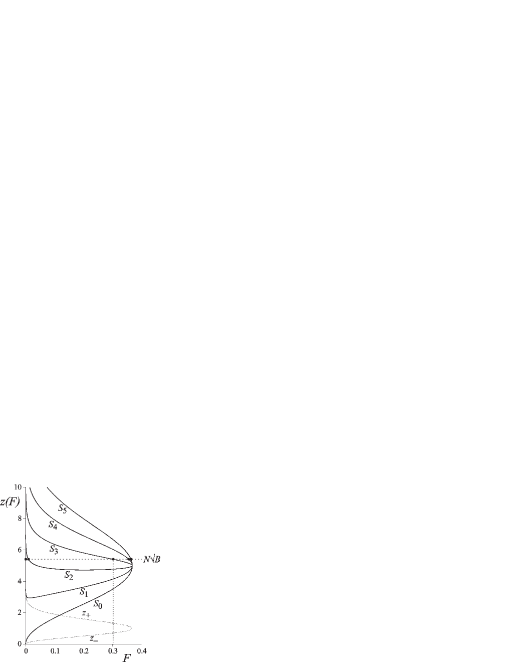
Figure 2: Inverted flux functions $z_{-}(F)$ and $z_{+}(F)$ and the $N+1$ sumfunctions $S_{m}(F)=mz_{+}(F)+(N-m)z_{-}(F),m=0,1,\ldots,N$. Here we picked $N=5$. The points of intersection with the horizontal line $z=N\sqrt{B}$ represent the fixed points for the parameter value $B$. Curves $S_{0}$ and $S_{5}$ correspond to the uniform distribution (below and above the critical point $B=1$, respectively) and the other curves belong to clustered states. Note that $S_{0}$ joins smoothly with $S_{5}$ at $B=1$ (i.e. $z=N\sqrt{B}=5$), and so does $S_{1}$ with $S_{4}$, and $S_{2}$ with $S_{3}$.

First, the one-humped function $F(z)$ is inverted separately on both sides of the maximum, yielding the functions $z_{-}(F)$ and $z_{+}(F)$. Then, we construct the sumfunctions:

$$S_{m}(F)=m\,z_{+}(F)+(N-m)\,z_{-}(F)$$ (7)

Now, from Eq. (6), the fixed points are found by intersecting the horizontal line $z=N\sqrt{B}$ with the sumfunctions $S_{m}(F)$. In Fig. 2 this is done for $B$=1.08. Each intersection point yields a pair $\{z_{-},z_{+}\}$, or equivalently $\{n_{-},n_{+}\}$. Repeating the procedure for all $B$, we obtain the bifurcation diagram depicted in Fig. 3.

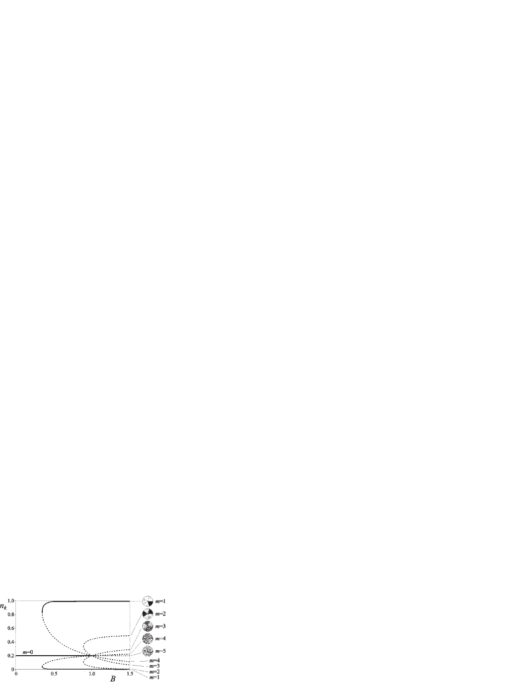
Figure 3: Bifurcation diagram for $N=5$. It has been obtained from Fig. 2 by converting, for all $B$, each $\{z_{-},z_{+}\}$-pair belonging to a point of intersection to a $\{n_{-},n_{+}\}$-pair. Note that all branches come together at the critical point $B=1$. The (stable) $m=0$ branch becomes the (unstable) $m=5$ branch, the $m=1$ branch turns into the $m=4$ branch, and $m=2$ switches to $m=3$.

It contains several branches. First, a horizontal line (from the sumfunctions $S_{0}$ and $S_{5}$) corresponding to the equal distribution $n_{+}=n_{-}=0.2=1/N$. Second, the branches corresponding to the $m=1$ clustered state (from $S_{1}$), which at $B=1$ goes over into the $m=4$ state (from $S_{4}$). And third, the branch of the $m=2$ clustered state (from $S_{2}$), which at $B=1$ becomes the $m=3$ state. The physical appearance of these solutions is sketched in the small diagrams. Note that only the $m=0$ branch (i.e., the uniform solution up to $B=1$) and the outer $m=1$ branch are stable. All the other branches are unstable, as will be discussed in the next section.

At $B=1$, where the branches intersect with the uniform distribution $n_{+}=n_{-}=1/N$, we have a critical point. In the flux function one passes the maximum here. This means that $n_{+}$ and $n_{-}$ are switched (relatively empty compartments become relatively filled, and vice versa), so $m$-branches change into $(N-m)$-branches. From a physical point of view, the most important thing that happens at the $B=1$ intersection point is the destabilization of the uniform distribution.

The saddle-node bifurcations of the $m=1$ and $m=2$ branches correspond to the minima of the sumfunctions $S_{1}$ and $S_{2}$ respectively, which in Fig 2 can be seen to occur at $F\approx 0.014$ for $S_{1}$ and $F\approx 0.202$ for $S_{2}$. In general, if a sumfunction $S_{m}(F)$ has a minimum for a certain $B$, the associated $m$ branch will have a bifurcation. So the bifurcation condition is that the derivative $dS_{m}(F)/dF$ equals zero, or equivalently:

$$\frac{\left(\dfrac{dz_{-}}{dF}\right)}{\left(\dfrac{dz_{+}}{dF}\right)}=-\frac{m}{N-m}$$ (8)

Not surprisingly, the quantity on the left hand side ($dz_{-}/dz_{+}\equiv\sigma$) will play an important role in the stability analysis of the next section.

III Stability of the branches

The stability of the branches (i.e., of the fixed points) is determined by the eigenvalues of the Jacobi matrix $\mathbf{J}$ corresponding to Eq. (4), with components:

$$J_{jk}=\frac{\partial\dot{n}_{j}}{\partial n_{k}}=\sum_{l}M_{jl}F^{\prime}(n_{l})\frac{\partial n_{l}}{\partial n_{k}}=M_{jk}F^{\prime}(n_{k})$$ (9)

Here $F^{\prime}$ denotes the derivative of $F$ with respect to $n$. Note that the Jacobi matrix can also be written as the product of $\mathbf{M}$ and the diagonal matrix $\mathbf{D}=\operatorname{diag}(F^{\prime}(n_{1}),\ldots,F^{\prime}(n_{N}))$, see also Eq. (18) in the Appendix. For a fixed point the only diagonal elements that occur are $F^{\prime}(n_{+})$ ($m$ times) and $F^{\prime}(n_{-})$ ($N-m$ times), in any order. The ratio between these two functions is precisely the quantity we encountered earlier in the bifurcation condition Eq. (8), namely $\sigma$:

$$\sigma=\frac{F^{\prime}(n_{+})}{F^{\prime}(n_{-})}=\frac{dn_{-}}{dn_{+}}$$ (10)

The Jacobi matrix $\mathbf{J}$ has $N$ eigenvalues, one of which is always zero. The other $N-1$ eigenvalues depend on $m$ and the value of $\sigma$.

For $m=0$ (the equipartitioned state) all non-trivial eigenvalues are negative, up to the point $B=1$. This can be seen either by direct numerical calculation, or analytically (see Appendix). At $B=1$, the $m=0$ state becomes the $m=N$ state. Here, the functions $F^{\prime}$ in the Jacobi matrix (9) change sign, and so do all of its eigenvalues. So suddenly the uniform state has $N-1$ positive eigenvalues, which implies a high degree of instability. Only in the limit $B\to\infty$ does the uniform state regain some of the lost terrain: the magnitude of all positive eigenvalues tends to zero here. Physically speaking, in this limit the vibro-fluidization is too weak to drive the particles out of the boxes anymore.

As for the other values of $m$, in Fig. 4 we have plotted the numerically evaluated eigenvalues (as functions of $\sigma$) for the system with $N=5$ compartments.

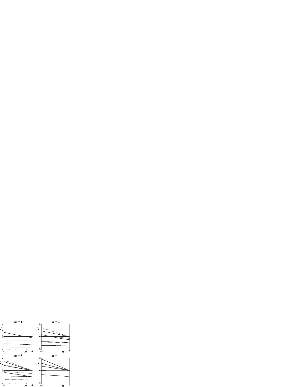
Figure 4: Eigenvalues of the Jacobi matrix $\mathbf{J}$ as a function of $\sigma$, for the branches $m$ = 1, 2, 3, and 4. Rather than plotting $\lambda_{i}$, we display $\tilde{\lambda}_{i}=\lambda_{i}/F^{\prime}(n_{-})$, because this yields a more clear-cut picture. Negative eigenvalues represent stable directions of the branches, and positive eigenvalues represent unstable ones. A zero crossing (such as for $m=1$ and $m=2$) indicates the occurrence of a saddle-node bifurcation. The value $\sigma=0$ corresponds to the limit $B\to\infty$, and $\sigma=-1$ to the critical point $B=1$. At this point, the eigenvalues of $m=1$ and $m=4$ are equal but opposite in sign: the transition from the one branch to the other is marked by a distinct drop in stability. The same is true for the eigenvalues of $m=2$ and $m=3$, and also (not depicted) for those of $m=0$ and $m=5$. For $m$ = 2, 3 there are two different cluster-configurations, with different eigenvalues. The dashed lines correspond to $\{++---\}$ for $m=2$, which goes over into $\{--+++\}$ for $m=3$. The bold lines apply to the slightly more stable configurations $\{+-+--\}$ and $\{-+-++\}$.

For $m=1$, we see that there are three eigenvalues that are always negative. The fourth non-trivial eigenvalue changes sign at $\sigma=-0.25$. This corresponds to the saddle-node bifurcation of the $m=1$ branch in the bifurcation diagram (Fig. 3), and the bifurcation value of $\sigma$ is in agreement with Eq. (8). The region to the right of $\sigma=-0.25$ (where all non-trivial eigenvalues are negative) belongs to the stable outer branch. The left part $\sigma<-0.25$ belongs to the unstable inner branch, up to the point $B=1$ (at $\sigma=-1$), where the $m=1$ branch goes over into the $m=4$ branch. That is, the state $\{+----\}$ now switches to $\{-++++\}$. At the same time all eigenvalues change sign, so suddenly we have $3$ positive eigenvalues, which is only one less than for the uniform $m=5$ state. (Indeed, the only stable manifold of the $m=4$ fixed point comes from the direction of the completely unstable $m=5$ state). The positive eigenvalues never cross zero anymore (there are no bifurcations beyond $B=1$) but, as before, in the limit $B\to\infty$ ($\sigma\to 0$) they go to zero.

For $m=2$ there are two possible configurations: $\{++---\}$ and $\{+-+--\}$. Due to the cyclic symmetry, all other combinations are equivalent to these two. The eigenvalues of the first configuration are given by the dotted lines, and those of the second by the solid lines. Although they are very similar (and are represented by exactly the same branch in the bifurcation diagram), it is clear that the second configuration is the more stable of the two. Apparently the two well-filled compartments prefer to keep a distance.

The saddle-node bifurcation of the $m=2$ branch takes place at $\sigma=-2/3$ [cf. Eq. (8)], where the third non-trivial eigenvalue goes through zero. The fourth non-trivial eigenvalue always remains positive, indicating that the $m=2$ branch never becomes completely stable. (As a matter of fact, only the $m=0$ branch and part of the $m=1$ branch can be completely stable). Note that for $\sigma\to 0$ (large $B$) the positive eigenvalue tends to zero, so the degree of instability is quite weak there.

At $B=1$ the $m=2$ branch becomes the $m=3$ branch, with the two configurations $\{--+++\}$ and $\{-+-++\}$, and with all eigenvalues switching sign. As we see, the more dispersed configuration is again the less unstable one. Also the phenomenon of all positive eigenvalues going to zero as $\sigma$ approaches zero (the weak driving limit $B\to\infty$) is again apparent.

In the present example for $N=5$, and in fact for all odd values of $N$, the branches in the bifurcation diagram are all born by means of a saddle-node bifurcation. But for even values of $N$ this is different: in that case there is one branch-pair that springs from the uniform distribution, at $B=1$, by a pitchfork bifurcation. This is illustrated in Fig. 5 for $N=6$. Here one sees all the branches that were present already for $N=5$, only slightly shifted towards the left, plus an additional pair of branches ($m=3$) bifurcating in the forward direction from $B=1$.

Figure 5: Bifurcation diagram for $N=6$. Note the pitchfork bifurcation at $B=1$.

The special status of the branch $m=N/2$ is also evident from Eq. (8), which tells us that the bifurcation condition for this branch is $\sigma=-1$. This condition is fulfilled only by $n_{+}=n_{-}=1/\sqrt{B}=1/N$. So, unlike all other branches, this one originates at $B=1$ from the (until then stable) uniform state. Related to this, the branch is the only one that is symmetric for interchanging $n_{+}$ and $n_{-}$.

IV Physical aspects

The bifurcation analysis from the previous section can also be understood from a more physical point of view. To this end, let us first have a closer look at a 2-box system. In the equilibrium situation the net flux between the two boxes is zero, with one filled ($n_{+}$) and one nearly empty ($n_{-}$) box. Suppose the level of the empty box is raised by an amount $\delta n$. The level of the filled box then decreases by an equal amount and the net flux $\phi_{-\to+}$ from the empty to the filled box becomes (see also Fig. 1):

$$\phi_{-\to+} =F(n_{-}+\delta n)-F(n_{+}-\delta n)$$ (11)

$$=\left(\frac{dF}{dn_{-}}+\frac{dF}{dn_{+}}\right)\delta n=\left(1+\sigma\right)\frac{dF}{dn_{-}}\delta n$$

where we have used that $\sigma=dn_{-}/dn_{+}$ and neglected the higher order terms in the Taylor expansion. There are two different regimes. If $\sigma>-1$, the net flux is positive (as $F^{\prime}(n_{-})$ is always positive), so particles are flowing from $n_{-}$ to $n_{+}$, restoring the equilibrium position. This is actually the situation along the entire $m=1$ branch, for all $1<B<\infty$. For $\sigma<-1$ (a situation which does not occur for our choice of $F$), the net flux would be negative, raising the level of the emptier box even further, away from the equilibrium position. In the borderline case, $\sigma=-1$ (at $B=1$), the system is indifferent to infinitesimal changes.

This argument is readily generalized to the $N$-compartment system, for an equilibrium with $m$ filled boxes. Now we raise the level of all $N-m$ nearly empty boxes simultaneously by $\delta n$. This is done by lowering all levels in the $m$ filled boxes by an equal amount, which by particle conservation must be equal to $\delta n(N-m)/m$. The equivalent of Eq. (11) for the flux between any of the empty boxes to a neighbouring filled box then reads:

$$\phi_{-\to+} =F(n_{-}+\delta n)-F(n_{+}-\frac{N-m}{m}\delta n)$$ (12)

$$=\left(\frac{dF}{dn_{-}}+\frac{N-m}{m}\frac{dF}{dn_{+}}\right)\delta n$$

$$=\left(\frac{m}{N-m}+\sigma\right)\frac{dF}{dn_{-}}\delta n$$

From this expression it follows that the transition between a (relatively) stable ($\sigma>-m/(N-m)$) and a (relatively) unstable ($\sigma<-m/(N-m)$) configuration is marked by the bifurcation condition Eq. (8). So, by straightforward physical reasoning we have reproduced the exact result obtained earlier from an eigenvalue analysis.

The pitchfork bifurcation discussed at the end of Section III is especially important for $N=2$. In this case it is the only non-uniform branch. To be specific, it is a stable $m=1$ branch. This $N=2$ case eggers99 is the only one without any saddle-node bifurcations, and consequently it is the only case where the change from the uniform to the clustered situation takes place via a second order phase transition without any hysteresis. For all $N>2$ the transition is of first order vdweele00 , and shows a hysteretic effect that becomes more pronounced for growing $N$.

In the limit $N\to\infty$ the hysteresis is maximal: the first saddle-node bifurcation takes place immediately after $B=0$, and this means that there exists a stable $m=1$ solution over the entire range $B>0$. So, if one starts out from this solution (at a certain value of $B$) and then gradually turns down $B$, one will never witness the transition to the uniform distribution. Vice versa, also the transition from the uniform solution to the $m=1$ state will not occur in practice, even though the uniform distribution becomes unstable at $B=1$. If one starts out from the uniform solution (at a certain value of $B$ below 1) and increases $B$, one will witness the transition to a clustered state, but in practice this will always be one with a number of peaks. That is, the system gets stuck in a transient state with $m>1$, even though such a state is not stable (it has one or more positive eigenvalues).

The fact is that its lifetime may be exceedingly large, since the flux in the neighborhood of a peak and its adjacent boxes (which are practically empty) is very small. Furthermore, the communication between the peaks is so poor that usually (even for moderate values of $N$) the dynamics comes to a standstill in a state with peaks of unequal height.

Another point we would like to address is that practically the transition to a clustered state will take place already before $B=1$, because the solution is kicked out of its basin of attraction by the statistical fluctuations in the system vdweele00 . An example is shown in Fig. 6. Here we see a snapshot for the cyclic system with $N=80$ compartments, which were originally filled almost uniformly, at $B=0.90$. The small random fluctuations in the initial condition are sufficient to break away from the (still stable) uniform distribution, and one witnesses the formation of a number of isolated clusters. In the further evolution these clusters deplete the neighbouring compartments and indeed the whole intermediate regions. But the peaks themselves, once they are well-developed, do not easily break down anymore.

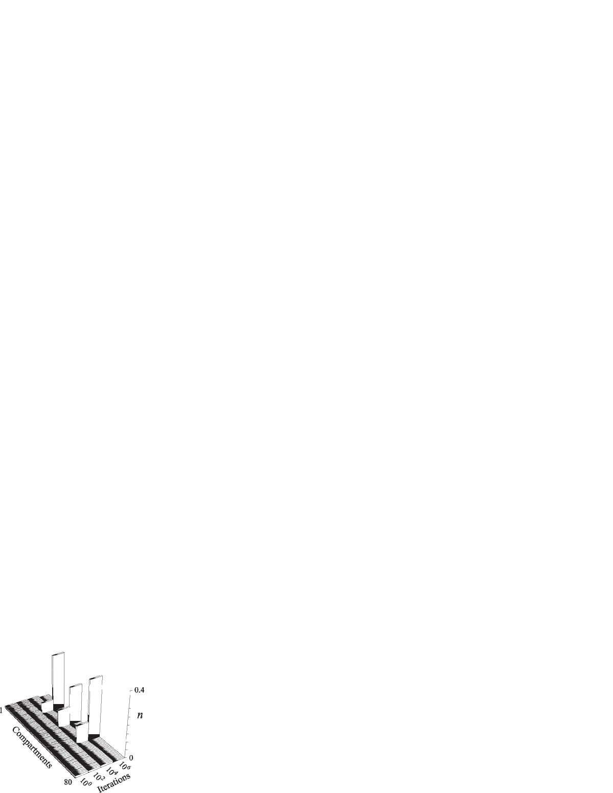
Figure 6: Results from a numerical solution of Eq. (4) for $N=80$, at $B=0.90$. Snapshots are taken after $10^{0}$, $10^{2}$, $10^{4}$ and $10^{6}$ timesteps (iterations). Between 100 and 10,000 iterations a clustering pattern is seen take shape. Although strictly speaking this is a transient state, the system gets stuck in it.

V Concluding remarks

In this paper we have constructed the bifurcation diagram for a vibro-fluidized granular gas in $N$ connected compartments. Let us now comment upon the result.

Starting out from $B=0$, i.e, vigorous shaking, the equi-partitioned state is for some time the only (and stable) fixed point of the system. For increasing $B$ we first come upon the $m=1$ bifurcation, where the single-cluster state is born. For all $N>2$ this happens by means of a saddle-node bifurcation, creating one completely stable state and one unstable state (with $1$ positive eigenvalue). The one with the largest difference between $n_{+}$ and $n_{-}$ is the stabler one of the two states. Strictly speaking, there are $N$ equivalent single-cluster states, since the cluster can be in any of the $N$ compartments.

For further growing $B$ we come across the $m=2$ bifurcation, where two unstable 2-peaked states are created. The state with the largest difference between $n_{+}$ and $n_{-}$ has $1$ positive eigenvalue, and the other one $2$. The two peaks can be distributed in $\binom{N}{2}$ ways over the $N$ compartments, but as we have seen they are not all equivalent. When the peaks are situated next to each other we have a more unstable situation (the positive eigenvalues are larger in magnitude) than when the peaks are further apart. This is generally true for $m$-peaked solutions: of the $\binom{N}{m}$ ways in which $m$ peaks can be distributed, the ones in which the peaks are next to each other are the least favorable of all.

For increasing $B$ we encounter more and more bifurcations, where unstable $m$-clustered states come into existence (each with $1$ more positive eigenvalue than the previous one), and for large $N$ the bifurcation diagram is covered by a dense web of branches. In Fig. 7 this is shown for N=80. The last saddle-node bifurcation takes place shortly before $B=1$ and, for this even value of $N$, is followed by a final pitchfork bifurcation (creating the $m=N/2$ branch) at $B=1$.

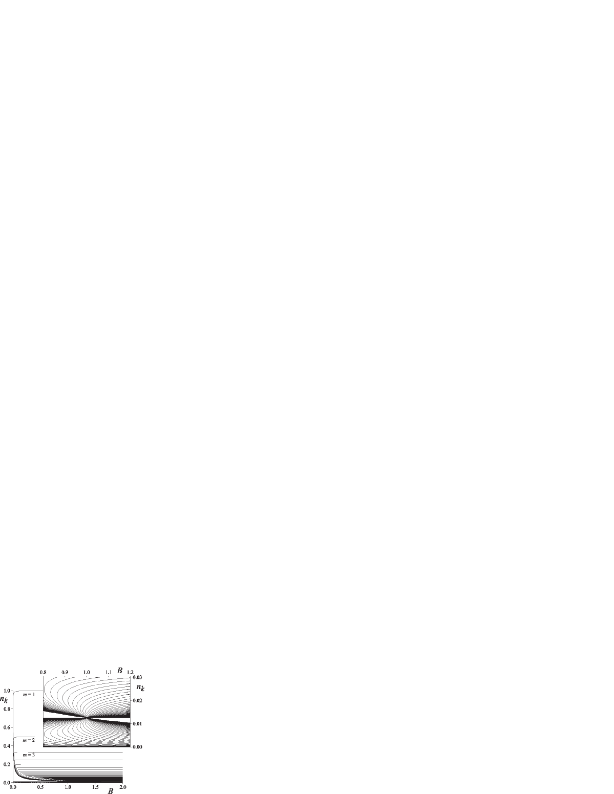
Figure 7: Bifurcation diagram for $N=80$. The hysteresis extends almost all the way down to $B=0$, and there are numerous transient states (cf. Fig. 6). The only strictly stable branches are the $m=0$ branch (up to $B=1$) at $n_{k}=1/N$, and the outer $m=1$ branches. Naturally, the upper $m=1$ branch approaches $n_{k}=1$, the upper $m=2$ branch approaches $n_{k}=1/2$, the upper $m=3$ branch $n_{k}=1/3$, etc. The overlay picture shows the neighborhood of the critical point at $B=1,n_{k}=1/N$ in more detail.

The uniform solution (or $m=0$ state) is stable until $B=1$, with $N-1$ negative eigenvalues and $1$ zero. For $B>1$ all its negative eigenvalues become positive, making it suddenly the most unstable state of all. Also, it now formally becomes the $m=N$ state. Moving away from this uniform solution one encounters first the $m=N-1$ branch with $N-2$ positive eigenvalues, then the $m=N-2$ branch with $N-3$ positive eigenvalues, etc. Finally, one arrives at the outermost $m=1$ branch, which has no positive eigenvalues. This is the only solution that is completely stable for $B>1$. But as we have seen in the previous section, on its way from the uniform distribution to the single peaked state, the system can easily get stuck in one of the transient states (especially for large $N$) even though these are not strictly stable.

Throughout the paper, we have concentrated on the case where the $N$ compartments are arranged in a cyclic manner. But in doing so, we have in fact also solved the non-cyclic case. Here we close the hole in the wall between the $1$st and $N$th compartment, and consequently the flux between them is zero. The matrix $\mathbf{M}$ then takes the following form [differing from the cyclic one only in the first and last row, cf. Eq. (4)]:

$$\mathbf{M}^{(nc)}=\left(\begin{smallmatrix}-1&1&0&0&\cdots&0&0\\ 1&-2&1&0&\cdots&0&0\\ 0&1&-2&1&\cdots&0&0\\ :&:&:&:&&:&:\\ :&:&:&:&&:&:\\ 0&0&0&0&\cdots&-2&1\\ 0&0&0&0&\cdots&1&-1\end{smallmatrix}\right)$$ (13)

The eigenvalue problem for this matrix is treated in the Appendix. One eigenvalue is identically zero, and the other $N-1$ eigenvalues are negative, just like for the cyclic system. This leads to a bifurcation diagram that is indistinguishable from that of the cyclic case. Even the stability along the branches is the same; only the magnitude (not the sign) of the eigenvalues of the Jacobi-matrix $\mathbf{J}$ is slightly different for the two cases.

Finally, it should be emphasized that the results of the present paper do not depend on the precise form of the flux function. We have concentrated on the form given by Eq. (1), but virtually everything remains true for other choices of this function, as long as it is a non-negative, one-humped function, starting out from zero at $n=0$ (no flux if there are no particles) and going down to zero again for very many particles (no flux also in this limit, since - due to the inelastic collisions - the particles form an inactive cluster, unable to reach the hole in the wall anymore). Any function with these properties will produce a bifurcation diagram similar to that of Eq. (1).

In the likely case that the range of $\sigma=dn_{-}/dn_{+}$ is the same, extending from $-1$ (this value is attained in the maximum) to zero (in the outer regions of the flux function, for $n_{-}\sqrt{B}\to 0$, $n_{+}\sqrt{B}\to\infty$), the bifurcation diagram will have the same number of saddle-node bifurcations and the same number of branches. The only things that change are the exact position of the bifurcation points, and the magnitude of the eigenvalues along the branches.

Slight differences in the diagram would occur if the slope of $F$ on the $n_{+}$ side was to become steeper than on the $n_{-}$ side. In that case, the bifurcation condition Eq. (8) would also have solutions for $m>N/2$, thus allowing saddle-node bifurcations for branches with $m>N/2$. These branches, however, would certainly be quite unstable.

APPENDIX: On the eigenvalues of $\mathbf{M}$ and $\mathbf{J}$

In this appendix we present the analytical eigenvalues of the flux matrix $\mathbf{M}$ [introduced in Eqs. (4) and (13)] and discuss the eigenvalue problem for the Jacobian matrix $\mathbf{J}$ [see Eq. (9)], thereby determining the stability of the branches in the bifurcation diagram.

First, we briefly treat the eigenvalues of $\mathbf{M}$. After that, we turn to $\mathbf{J}$. In Subsection 2 we discuss its zero-eigenvalues: one eigenvalue is identically zero and, by pinpointing the zero-crossing of a second eigenvalue, we reproduce the bifurcation condition Eq. (8). In Subsection 3 we determine the number of negative eigenvalues of $\mathbf{J}$ in the low-driving limit $\sigma\to 0$. Likewise, in Subsection 4 we determine the number of positive eigenvalues in the (mathematical) limit $\sigma\to-\infty$. Combining these two results, in Subsection 5, we finally find the number of positive eigenvalues of $\mathbf{J}$ for general values of $\sigma$, and this gives the stability of the branches over the entire bifurcation diagram.

.1 Eigenvalues of matrix $\mathbf{M}$

The matrix $\mathbf{M}$ in Eq. (4) is closely related to the $N\times N$ tridiagonal matrix $\operatorname{tridiag}(1,-2,1)$ associated with the second difference operator known from numerical schemes for solving second order pde’s. Its eigenvalue problem can be solved exactly guardiola82 , and the same is true for $\mathbf{M}$. The eigenvalues of $\mathbf{M}$ are given by:

$$\lambda_{k}=-4\sin^{2}\left(\frac{k\pi}{N}\right)$$ (14)

where $k$ runs from $0$ to $N/2$ for $N$ even, and from $0$ to $(N-1)/2$ for $N$ odd. The corresponding eigenvectors are:

$$a_{i}(k)=C_{1}\cos\left(\frac{(2i+1)k\pi}{N}\right)+C_{2}\sin\left(\frac{(2i+1)k\pi}{N}\right)$$ (15)

with $i=1,\ldots,N$ and arbitrary coefficients $C_{1}$ and $C_{2}$.

As we see, the first eigenvalue ($k=0$) is zero and the corresponding eigenvector is $\mathbf{1}=(1,1,\ldots,1)$. Physically, this eigenvector represents simultaneous filling of all $N$ compartments, and the eigenvalue $0$ expresses the fact that this is prohibited (because the number of particles in our system is conserved).

All non-zero eigenvalues are negative and (except the one for $k=N/2$ in the case of even $N$) doubly degenerate. This means that the corresponding eigenvectors span a two-dimensional subspace, reflected by the two terms $C_{1}$ and $C_{2}$ in Eq. (15). Since $\mathbf{M}$ is symmetric, and therefore normal, linear subspaces corresponding to different eigenvalues are orthogonal. Especially, the eigenvectors of all non-zero eigenvalues span a $N-1$ dimensional subspace perpendicular to $\mathbf{1}=(1,1,\ldots,1)$.

The matrix $\mathbf{M}^{(nc)}$ for the non-cyclic case, given by Eq. (13), has a different set of eigenvalues:

$$\lambda^{(nc)}_{k}=-4\sin^{2}\left(\frac{k\pi}{2N}\right)$$ (16)

Here $k$ runs from $0$ to $N-1$. The corresponding eigenvectors are:

$$a^{(nc)}_{i}(k)=\cos\left(\frac{(2i+1)k\pi}{2N}\right)$$ (17)

Just like in the cyclic case, the first eigenvalue equals zero, and all the others are negative. However, they are non-degenerate and the corresponding eigenspaces are one-dimensional.

.2 Zero-eigenvalues of matrix $\mathbf{J}$

Now we turn to the Jacobian matrices. We consider the cyclic version $\mathbf{J}$, with components as given in Eq. (9), but the results are also valid for the non-cyclic version. This matrix can be written as the product of $\mathbf{M}$ and a diagonal matrix $\mathbf{D}=\operatorname{diag}(F^{\prime}(n_{1}),F^{\prime}(n_{2}),\ldots,F^{\prime}(n_{N}))$:

$$\mathbf{J}=\mathbf{M}\cdot\mathbf{D}=\left(\begin{smallmatrix}-2F^{\prime}(n_{1})&F^{\prime}(n_{2})&0&\cdots&0&F^{\prime}(n_{N})\\ F^{\prime}(n_{1})&-2F^{\prime}(n_{2})&F^{\prime}(n_{3})&\cdots&0&0\\ 0&F^{\prime}(n_{2})&-2F^{\prime}(n_{3})&\cdots&0&0\\ :&:&:&&:&:\\ :&:&:&&:&:\\ 0&0&0&\cdots&-2F^{\prime}(n_{N-1})&F^{\prime}(n_{N})\\ F^{\prime}(n_{1})&0&0&\cdots&F^{\prime}(n_{N-1})&-2F^{\prime}(n_{N})\end{smallmatrix}\right)$$ (18)

In the context of the bifurcation diagram, the main thing one wants to know is the number of positive eigenvalues of $\mathbf{J}$ for each branch. This is what we are going to determine now.

First we note that the eigenvalues of $\mathbf{J}$ are real, even though the matrix is not symmetric. This is a consequence of the following similarity relationship between $\mathbf{J}$ and $\mathbf{J}^{{\dagger}}$:

$$\mathbf{J}^{{\dagger}}=(\mathbf{M}\cdot\mathbf{D})^{{\dagger}}=\mathbf{D}\cdot\mathbf{M}=\mathbf{D}\cdot(\mathbf{M}\cdot\mathbf{D})\cdot\mathbf{D}^{-1}=\mathbf{D}\cdot\mathbf{J}\cdot\mathbf{D}^{-1}$$ (19)

This implies that $\mathbf{J}$ and $\mathbf{J}^{{\dagger}}$ have the same eigenvalues, and hence they must be real. Because $\mathbf{M}$ is singular, $\mathbf{J}$ must be too (it has a zero eigenvalue) and so its determinant $\det(\mathbf{J})$ is zero. More explicitly:

$$\det(\mathbf{J})=\det(\mathbf{M})\cdot\det(\mathbf{D})=\left(\prod_{k}F^{\prime}(n_{k})\right)\det(\mathbf{M})=0$$ (20)

where, for a fixed point with $m$ filled compartments, the product term equals $[F^{\prime}(n_{+})]^{m}[F^{\prime}(n_{-})]^{(N-m)}$.

For the other eigenvalues we have to look at the characteristic equation $\det(\mathbf{J}-\lambda\mathbf{I})=0$. This is a polynomial expression in $\lambda$, of which the constant term is zero since it is equal to $\det(\mathbf{J})$. The coefficient $L$ of the linear term is:

$$L=\sum_{k}\det(\mathbf{J}^{(k,k)})=\sum_{k}\left(\prod_{l\neq k}\lambda_{l}\right)$$ (21)

where the matrix $\mathbf{J}^{(k,k)}$ is the $(N-1)\times(N-1)$ matrix obtained from $\mathbf{J}$ by deleting its $k$-th row and its $k$-th column. In the right-hand side of this equation, the only product that survives is the one that does not contain the trivial (zero) eigenvalue. So:

$$L=\prod_{\text{all non-trivial}\lambda_{l}}\lambda_{l}$$ (22)

Alternatively, the determinant of $\mathbf{J}^{(k,k)}$ in Eq. (21) can be written in terms of $\det(\mathbf{M}^{(k,k)})$, by deleting the $k$-th factor from the product in Eq. (20):

$$L=\sum_{k}\left(\prod_{l\neq k}F^{\prime}(n_{l})\right)\det(\mathbf{M}^{(k,k)})$$ (23)

It can be shown that for all $k$ the determinant $\det(\mathbf{M}^{(k,k)})$ is a constant, $C$, which equals $(N-1)(-1)^{N-1}$ in the cyclic, and $(-1)^{N-1}$ in the non-cyclic case. Thus, Eq. (23) reduces to:

$$L=C\sum_{k}\left(\prod_{l\neq k}F^{\prime}(n_{l})\right)$$ (24)

For a fixed point with $m$ filled compartments, we can write (using that in the above summation each of the products misses either an $F^{\prime}(n_{+})$ or an $F^{\prime}(n_{-})$):

$$L =C[F^{\prime}(n_{+})]^{(m-1)}[F^{\prime}(n_{-})]^{(N-m-1)}\times$$ (25)

$$\quad\quad\quad\Big{(}(N-m)F^{\prime}(n_{+})-mF^{\prime}(n_{-})\Big{)}$$

$$=C[F^{\prime}(n_{+})]^{(m-1)}[F^{\prime}(n_{-})]^{(N-m)}\Big{(}(N-m)\sigma-m\Big{)}$$

From this equation we conclude that $L$ becomes zero at $\sigma=-m/(N-m)$. This is exactly the bifurcation condition already given in the main text [Eq. (8)]. Also, with Eq. (22), we see that an eigenvalue crosses zero at this value of $\sigma$.

It can be shown, by a similar analysis, that the coefficient of the quadratic term is not equal to zero at $\sigma=-m/(N-m)$, so not more than one of the eigenvalues changes sign at the bifurcation.

.3 Number of negative eigenvalues of $\mathbf{J}$ for $\sigma\to 0$

We now come to the next step in determining the number of positive eigenvalues. We again use the definition of $\sigma$ to write: $\mathbf{J}=F^{\prime}(n_{-})\mathbf{M}\cdot\mathbf{\widetilde{D}}$, where $\mathbf{\widetilde{D}}=\operatorname{diag}(1,\ldots,1,\sigma,\ldots,\sigma)$. The factors $1$ correspond to the $N-m$ nearly empty boxes and the factors $\sigma$ to the $m$ filled boxes. The precise ordering of the factors is not essential for the following argument, so we may choose the above order for notational convenience.

The factor $F^{\prime}(n_{-})$ is always positive, so we only have to deal with $\mathbf{M}\cdot\mathbf{\widetilde{D}}$. Note that only $\mathbf{\widetilde{D}}$ depends on $\sigma$ and that in the limit $\sigma\to 0$ this matrix becomes:

$$\lim_{\sigma\to 0}\mathbf{\widetilde{D}}=\operatorname{diag}(1,\ldots,1,0,\ldots,0)\equiv\mathbf{P}$$ (26)

$\mathbf{P}$ is a projection matrix which projects $\mathbb{R}^{N}$ to the subspace spanned by the first $N-m$ unit vectors. It is obviously non-singular, symmetric, and applying it twice gives the same result as once: $\mathbf{P}^{2}=\mathbf{P}$.

Instead of taking the matrix $\mathbf{J}_{0}=\mathbf{M}\cdot\mathbf{P}$ as input for solving our eigenvalue problem (in the limit $\sigma\to 0$), we will rather look at the matrix $\mathbf{P}\cdot\mathbf{M}\cdot\mathbf{P}$ which is symmetric and has the same eigenvalues as $\mathbf{J}_{0}$.

For proof of the last statement, let $\mu$ be a (non-zero) eigenvalue of $\mathbf{J}_{0}$: $\mathbf{J}_{0}\cdot\mathbf{x}=\mu\mathbf{x}$. Then: $(\mathbf{P}\cdot\mathbf{M}\cdot\mathbf{P})\cdot(\mathbf{P}\cdot\mathbf{x})=\mathbf{P}\cdot(\mathbf{M}\cdot\mathbf{P}\cdot\mathbf{x})=\mu(\mathbf{P}\cdot\mathbf{x})$. Note that $\mathbf{P}\cdot\mathbf{x}\neq 0$, because otherwise also $\mathbf{J}_{0}\cdot\mathbf{x}=\mathbf{M}\cdot\mathbf{P}\cdot\mathbf{x}$ would be zero, contradicting the assumption that $\mu$ is non-zero. This completes the proof.

The matrix $\mathbf{M}$ is negative semi-definite. This means that $\mathbf{M}$ has only negative or zero eigenvalues or, equivalently, the inner product $\langle\mathbf{x},\mathbf{M}\cdot\mathbf{x}\rangle\leq 0$ for all $\mathbf{x}$. This means that also $\mathbf{P}\cdot\mathbf{M}\cdot\mathbf{P}$ is negative semi-definite, because:

$$\langle\mathbf{x},\mathbf{P}\cdot\mathbf{M}\cdot\mathbf{P}\cdot\mathbf{x}\rangle=\langle\mathbf{P}\cdot\mathbf{x},\mathbf{M}\cdot(\mathbf{P}\cdot\mathbf{x})\rangle=\langle\mathbf{y},\mathbf{M}\cdot\mathbf{y}\rangle\leq 0$$ (27)

In conclusion, $\mathbf{J}_{0}$ has negative and zero eigenvalues only.

The remaining task is to identify the number of negative eigenvalues, or otherwise stated, the rank of the matrix $\mathbf{J}_{0}$. The statement which we shall prove is that $\operatorname{rank}(\mathbf{J_{0}})=\operatorname{rank}(\mathbf{P})=N-m$.

Proof: Note that the image $\operatorname{Im}(\mathbf{P})$ of $\mathbf{P}$ is spanned by the first $m$ unit vectors of $\mathbb{R}^{N}$. Its kernel $\operatorname{Ker}(\mathbf{P})$ is spanned by the remaining $N-m$ unit vectors. Since the kernel of $\mathbf{M}$ is spanned by the vector $\mathbf{1}$, the following identities hold:

$$\operatorname{Ker}(\mathbf{P})\cap\operatorname{Ker}(\mathbf{M})=\mathbf{0}$$ (28a)

$$\operatorname{Im}(\mathbf{P})\cap\operatorname{Ker}(\mathbf{M})=\mathbf{0}$$ (28b)

Now, for all $\mathbf{x}\in\operatorname{Ker}(\mathbf{P})$ it holds that $\mathbf{J}_{0}\cdot\mathbf{x}=\mathbf{M}\cdot(\mathbf{P}\cdot\mathbf{x})=\mathbf{0}$, so $\operatorname{Ker}(\mathbf{P})\subset\operatorname{Ker}(\mathbf{J}_{0})$. On the other hand, for all $\mathbf{y}\notin\operatorname{Ker}(\mathbf{P})$ one has $\mathbf{P}\cdot\mathbf{y}\equiv\mathbf{z}\neq 0$, with $\mathbf{z}\in\operatorname{Im}(\mathbf{P})$, and therefore $\mathbf{J}_{0}\cdot\mathbf{y}=\mathbf{M}\cdot\mathbf{z}\neq 0$ because of Eq. (28b). This means that $\mathbf{y}\notin\operatorname{Ker}(\mathbf{J}_{0})$, and thus $\operatorname{Ker}(\mathbf{P})\supset\operatorname{Ker}(\mathbf{J}_{0})$. Together these two results prove that $\operatorname{Ker}(\mathbf{P})=\operatorname{Ker}(\mathbf{J}_{0})$, so obviously the rank of the two matrices must be equal. Since $\operatorname{rank}(\mathbf{P})=N-m$, this is also the rank of $\mathbf{J}_{0}$, which completes the proof.

In short, we have shown that in the limit $\sigma\to 0$, the Jacobi-matrix $\mathbf{J}$ has $N-m$ negative eigenvalues.

.4 Number of positive eigenvalues for $\sigma\to-\infty$

We now turn to the limit $\sigma\to-\infty$. In this limit we rewrite $\mathbf{J}$ as follows: $\mathbf{J}=F^{\prime}(n_{-})\sigma\mathbf{M}\cdot\mathbf{\bar{D}}$. Here $\mathbf{\bar{D}}=\operatorname{diag}(\sigma^{-1},\ldots,\sigma^{-1},1,\ldots,1)$, which in the limit $\sigma\to-\infty$ becomes:

$$\lim_{\sigma\to-\infty}\mathbf{\bar{D}}=\operatorname{diag}(0,\ldots,0,1,\ldots,1)\equiv\mathbf{Q}$$ (29)

Again, $\mathbf{Q}$ is a projection matrix, which now projects $\mathbb{R}^{N}$ to the subspace spanned by the last $m$ unit vectors, so $\mathbf{Q}$ is complementary to $\mathbf{P}$. Following the same line of reasoning, but keeping in mind that now the constant factor in front of $\mathbf{J}_{-\infty}$ is negative, we find that in the limit $\sigma\to-\infty$, the matrix $\mathbf{J}$ has $m$ positive eigenvalues.

.5 Number of positive eigenvalues of $\mathbf{J}$ for general $\sigma$

We are now ready to draw the conclusion. Just below $\sigma=0$ the matrix $\mathbf{J}$ must, by continuity, have at least $N-m$ negative eigenvalues. If we now move from $0$ towards $-\infty$, beyond a certain point there must be at least $m$ positive eigenvalues (or equivalently, at most $N-m-1$ negative eigenvalues). We already know [cf. Eq. (25)] that along the way exactly one eigenvalue changes sign, at $\sigma=-m/(N-m)$. Taken together, this means that $\mathbf{J}$ has $m$ positive and $N-m-1$ negative eigenvalues for $\sigma<-m/(N-m)$, and $m-1$ positive and $N-m$ negative eigenvalues for $\sigma>-m/(N-m)$.

This completes the determination of the number of positive eigenvalues for the various branches in the bifurcation diagram.

References

- (1) I. Goldhirsch and G. Zanetti, Phys. Rev. Lett. 70, 1619 (1993).
- (2) S. McNamara and W. Young, Phys. Rev. E 50, R28 (1994).
- (3) Y. Du, H. Li, and L. Kadanoff, Phys. Rev. Lett. 74, 1268 (1995).
- (4) H. Jaeger, S. Nagel, and R. Behringer, Rev. Mod. Phys. 68, 1259 (1996).
- (5) A. Kudrolli, M. Wolpert, and J. Gollub, Phys. Rev. Lett. 78, 1383 (1997).
- (6) L. Kadanoff, Rev. Mod. Phys. 71, 435 (1999).
- (7) J. Eggers, Phys. Rev. Lett. 83, 5322 (1999).
- (8) K. van der Weele, D. van der Meer, M. Versluis, and D. Lohse, Europhys. Lett. 53, 328 (2001).
- (9) S. McNamara and S. Luding, Phys. Rev. E 58, 813 (1998).
- (10) R. Guardiola and J. Ros, J. Comp. Phys. 45, 374 (1982).