Periodic orbit quantization of a Hamiltonian map on the sphere

Abstract

In a previous paper we introduced examples of Hamiltonian mappings with phase space structures resembling circle packings. It was shown that a vast number of periodic orbits can be found using special properties. We now use this information to explore the semiclassical quantization of one of these maps.

I Introduction

The general theory of periodic orbit quantization was first developed many years ago by Gutzwiller gutzwiller ; gutzwiller2 and has ever since played an important role in our understanding of chaotic systems in the semiclassical regime. By applying stationary phase approximations to the trace of the Green’s operator, Gutzwiller was able to derive a semiclassical formula for the density of states as the sum of a smooth part and an oscillating sum over all periodic orbits of the corresponding classical system. Gutzwiller’s ‘trace formula’, however, is only valid for isolated periodic orbits which, in general, restricts his results to fully chaotic systems where the dynamics is completely hyperbolic.

At the other end of the scale lie integrable systems. Armed with the knowledge of all constants of motion one may obtain the semiclassical eigenenergies using EBK torus quantization EBK . Alternatively, Berry and Tabor berry showed that EBK quantization could be recast as a ‘topological sum’ over the periodic orbits and obtained an analogue of Gutzwiller’s trace formula for integrable systems. The Berry-Tabor formula has also been extended into the near-integrable regime ozorio ; tomsovic . However most physical systems are of a mixed type, exhibiting both regular and chaotic behaviour. Some progress on the periodic orbit quantization of mixed systems has also been made sieber ; schomerus ; main3 .

The theory referred to above is for autonomous systems. The dynamics of periodically driven systems and quantum maps is best described by the so-called Floquet operator haake . Upon deriving an approximation for the trace of this unitary operator in terms of the classical periodic orbits, one may obtain a semiclassical approximation for the spectral density of its eigenphases. This trace formula has been derived for a class of maps on the plane tabor ; junker , on the torus laksh3 and for an array of special mappings with mixed results. The trace formula for Arnold’s cat map is exact keating ; boasman . However the more general sawtooth map gives poor results laksh3 ; laksh2 ; sano . It was found necessary to include boundary contributions in the trace formula of the baker’s map eckhardt ; saraceno ; laksh ; toscano ; tanner , while ghost contributions needed to be included in the case of the kicked top kus ; kus2 ; schomerus and the standard map scharf ; sundaram ; scharf2 ; saito . Poincaré maps have also been considered bogomolny .

The model for which we will apply Gutzwiller’s method of periodic orbit quantization is quite dissimilar to the above mappings. The dynamics of our model is dominated by an infinite number of isolated stable periodic orbits of arbitrarily long period. The resonances associated with these periodic orbits are circular disks and fill in the phase space in a manner resembling circle packings. Three of these mappings were introduced in a previous paper scott , each corresponding to a particular phase space geometry: planar, hyperbolic and spherical. We will consider only the spherical map in this paper. Its quantum analogue lives in a finite dimensional Hilbert space allowing us to circumvent convergence problems associated with semiclassical trace formulae main2 . In addition, our model does not suffer from the exponential proliferation of periodic orbits found in most chaotic systems. The task of finding all periodic orbits of a given period is much simplified with the help of symbolic labeling and the use of special symmetries. Our mapping is not chaotic in a strict sense. However the presence of infinitely many stable periodic orbits with arbitrarily long period generates highly irregular motion. This behaviour is located on the borderline between regular and chaotic motion, but in a manner very different from the generic case of KAM systems. The strong deviation is explained by the mapping’s non-smooth construction.

Our motivation for considering such a system is as follows. Tests of the applicability of periodic orbit quantization as a theory which adequately describes quantum systems in their semiclassical limit has, for the most part, been focussed on fully chaotic systems. Systems with regions of stability have been ignored due to complications in the theory which arise whenever non-isolated periodic orbits are present. For integrable systems, the presence of periodic tori surrounding each stable periodic orbit is accommodated in the theory of Berry and Tabor. However when such a system is perturbed into the near-integrable regime, these tori resonate and form island chains of high-order stable and unstable periodic orbits of equal period. If the perturbation is small, the newly created periodic orbits will not be sufficiently isolated, and hence, Gutzwiller’s theory cannot be applied. In such cases, uniform approximations need to be made which bridge the gap between the two theories ozorio ; tomsovic . For chaotic systems, each stable periodic orbit is locally near-integrable, and in general, will always be accompanied by island chains of non-isolated periodic orbits, which again inhibit the application of Gutzwiller’s theory. To explore the limits of periodic orbit quantization for the case of stable motion we need to first investigate ‘toy systems’ of low generality like ours where the method is expected to work best. The circular resonances associated with each stable periodic orbit of our mapping rotate about each point of the orbit in a linear fashion, and hence, contain no high-order resonances. For almost all parameter values, the period of rotation will be an irrational multiple of $\pi$. Thus, each stable periodic orbit will be isolated by the radius of its circular resonance, which, for a careful choice of the parameter values, can be made large enough such that Gutzwiller’s theory is applicable. The low generality of our model should not render our research as being futile or purely academic. Indeed, the investigation of other toy systems, such as Sinai’s billiard, has led to much insight for the hyperbolic case bohigas .

Our paper is sectioned as follows. In Section II we review the classical map and construct its generating function. For a more detailed exposition of the classical map one should refer to scott . In Section III we introduce the quantum map and spin coherent states. Using these states as a basis, we then derive semiclassical matrix elements of the Floquet operator in Section IV, followed by semiclassical traces and eigenphases in Section V. The theory in these sections follows the work by Kuś et al. kus . Numerical investigations of our semiclassical approximations are contained in sections VI and VII. Finally, in Section VIII we discuss our results.

II Classical map

The Hamiltonian under consideration is that of a kicked linear top

$$H({\bf J},t)=\omega J_{3}+\mu|J_{1}|\sum_{n=-\infty}^{\infty}\delta(t-n),$$ (1)

where $\mu,\omega\in[0,2\pi)$ are parameters and $({\bf J})_{i}=J_{i}=\epsilon_{ijk}x_{j}p_{k}$ $(i=1,2,3)$ are the three components of angular momentum for a particle confined to a sphere, normalized such that ${\bf J}\cdot{\bf J}=1$. The classical evolution of ${\bf J}$ is governed by the equations

$$\dot{J_{i}}=\{J_{i},H\},\quad\{J_{i},J_{j}\}=\epsilon_{ijk}J_{k}$$

where $\{\cdot\,,\cdot\}$ are the Poisson brackets. Their solution can be written as the mapping

$${\bf J}^{n+1}=\left[\begin{array}[]{c}J_{1}^{n+1}\\ J_{2}^{n+1}\\ J_{3}^{n+1}\end{array}\right]=\left[\begin{array}[]{ccc}\cos{\omega}&-\sin{\omega}&0\\ \sin{\omega}&\cos{\omega}&0\\ 0&0&1\end{array}\right]\left[\begin{array}[]{ccc}1&0&0\\ 0&\cos{\mu s^{n}}&-\sin{\mu s^{n}}\\ 0&\sin{\mu s^{n}}&\cos{\mu s^{n}}\end{array}\right]\left[\begin{array}[]{c}J_{1}^{n}\\ J_{2}^{n}\\ J_{3}^{n}\end{array}\right]\equiv\mbox{F}(s^{n}){\bf J}^{n}$$ (2)

where $s^{n}\equiv\,\mbox{sgn}\,J_{1}^{n}$, which takes ${\bf J}$ from just before a kick to one period later. Here $\,\mbox{sgn}\,x$ is the signum function with the convention $\,\mbox{sgn}\,0=0$.

The mapping is deceptively simple. It first rotates the eastern hemisphere ($J_{1}>0$) through an angle $\mu$ and the western hemisphere ($J_{1}<0$) through an angle $-\mu$. The great circle $J_{1}=0$ remains fixed. Then the entire sphere is rotated about the $J_{3}$ axis through an angle $\omega$. Thus the map rotates every point on the sphere in a piecewise linear fashion except on $J_{1}=0$ where its Jacobian is singular. Surprisingly, this leads to a phase space of great structural complexity. In Figure 1 we give examples for two different parameter values. The eastern hemisphere is shown in black, the western in gray. We will only consider the semiclassical quantization when $\mu=\omega=\pi(\sqrt{5}-1)$ as in Figure 1(b).

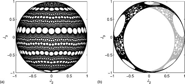
Figure 1: The phase space of the classical map when $\omega=\pi(\sqrt{5}-1)$ and (a) $\mu=0.02$, (b) $\mu=\omega$.

Note that if an orbit of our map does not have a point on $J_{1}=0$, then its Lyapunov exponents are zero, making it stable. If however, it does have a point on $J_{1}=0$, then its Lyapunov exponents are undefined. We overcome this problem by simply defining an unstable orbit to be one with a point on $J_{1}=0$, and all others stable. The unstable set is defined to be the closure of the set of all images and preimages of the great circle $J_{1}=0$. In figures 1 and 2 the unstable set is in black and gray. The circular holes are resonances consisting entirely of stable orbits. At their center lies a stable periodic orbit. It is these stable periodic orbits which will be used for the semiclassical quantization. All other points inside the resonances rotate about the central periodic orbit in a linear fashion. The period of rotation is an irrational multiple of $\pi$ for almost all values of the parameters $\mu$ and $\omega$, and hence, no other periodic orbits are located inside the resonances. In our case of study (Figure 1(b)), we have chosen $\mu$ to be large enough such that no island chains of first-order resonances form to create periodic quasi-tori (as in Figure 1(a)). Hence we have done our best to ensure that all of the stable periodic orbits are sufficiently isolated. The unstable periodic orbits are shown not to affect leading terms in the asymptotic analysis.

We have previously shown scott that it is possible to label every point of a stable periodic orbit of least period $n$ with a unique sequence $\{s^{k}=\pm 1\}_{k=1..n}$. The position of the point is given by the solution of

$${\bf J}=\mbox{F}(s^{n})\mbox{F}(s^{n-1})\dots\mbox{F}(s^{1}){\bf J}\equiv\mbox{R}{\bf J}$$ (3)

lying on the unit sphere with $\,\mbox{sgn}\,J_{1}=s^{1}$. The other $n-1$ points of the periodic orbit are found by substituting the $n-1$ cycles of the original sequence into (3). Hence, if $\{{\bf J}^{k}\}_{k=1..n}$ is a stable periodic orbit then the sequence corresponding to its first point is $\{\!\,\mbox{sgn}\,J_{1}^{k}\}_{k=1..n}$. Note that the (unnormalized) solution of (3) is simply the axis of rotation of R, namely

$${\bf J}=(\mbox{R}_{23}-\mbox{R}_{32}\,,\;\mbox{R}_{31}-\mbox{R}_{13}\,,\;\mbox{R}_{12}-\mbox{R}_{21}).$$

Although every periodic point is uniquely represented by a sequence, not every sequence represents a periodic point. Hence we still need to find which sequences are legitimate. This may be done by checking each of the $2^{n}$ different possible sequences for a period-$n$ orbit. However, this is computationally expensive for large periods. An alternative is to exploit symmetries of our mapping. We have previously conjectured scott that every stable periodic orbit has exactly one or two points on one of the following symmetry lines on the unit sphere:

$$J_{1} = -J_{2}\tan{\omega/2}$$

$$J_{2} = J_{3}\tan(\mu/2\,\mbox{sgn}\,J_{1})$$

$$J_{2} = J_{1}\tan{\omega/2}.$$

It is easy to prove that if a stable periodic orbit has one point on a particular symmetry line, then it has no more than two points on this line. However, we were not able to show that a stable periodic orbit must have a point on one of these lines, though numerical investigations suggest they do. We have checked all $2^{41}-2$ of the possible sequences for a stable periodic orbit of period $\leq 40$ and only found those of the above type. If one assumes our conjecture to be true then it is computationally easy to find all of the stable periodic orbits with periods upwards of 300 000. This may be done by finding where each symmetry line intersects with its image; an effortless task to solve numerically by virtue of the simplicity of our mapping. Every image of a symmetry line is just a collection of arc segments on the sphere. Once a periodic point is found, the size of its circular resonance can be calculated by noting that the resonance of at least one point of the orbit must touch $J_{1}=0$. This is because the boundary of each resonance forms part of the unstable set, and hence, iterates arbitrarily close to $J_{1}=0$. The sections of the symmetry line which intersect this periodic orbit’s resonances contain no other periodic orbits and may be ignored for the remainder of our search.

Following Kuś et al. kus we rewrite the map in terms of the complex variables $\gamma$ and $\gamma^{*}$

$$\gamma_{n+1}^{\phantom{*}}=e^{i\omega}\frac{\gamma_{n}^{\phantom{*}}-is^{n}\tan{\frac{\mu}{2}}}{1-i\gamma_{n}^{\phantom{*}}s^{n}\tan{\frac{\mu}{2}}}\equiv\Gamma(\gamma_{n}^{\phantom{*}},\gamma_{n}^{*})$$ (4)

where

$$\gamma\equiv\frac{J_{1}+iJ_{2}}{1+J_{3}}=e^{i\phi}\tan\frac{\theta}{2}$$

is the stereographic projection of the unit sphere ${\bf J}=(\sin\theta\cos\phi,\sin\theta\sin\phi,\cos\theta)$ onto the complex plane. We then construct its generating function ($\,\text{Re}\,\gamma\neq 0$)

$$W(\Gamma^{*},\gamma)=\log\left[(1+\gamma)(1+e^{i\omega}\Gamma^{*})+e^{i\mu s}(1-\gamma)(1-e^{i\omega}\Gamma^{*})\right]+C$$ (5)

where $s=\,\mbox{sgn}\,\!\,\text{Re}\,\gamma$ and $C$ is an arbitrary constant. The mapping $\Gamma(\gamma,\gamma^{*})$ can be rederived via the relations

$$\frac{\partial W}{{\partial\Gamma}^{*}}=\frac{\Gamma}{1+{\Gamma\Gamma}^{*}}\qquad\frac{\partial W}{\partial\gamma}=\frac{\gamma^{*}}{1+\gamma\gamma^{*}}.$$ (6)

It has been shown kus that for nearly any area preserving map $\Gamma(\gamma,\gamma^{*})$ it is possible to find a generating function $W(\Gamma^{*},\gamma)$ with $\gamma$ and $\Gamma^{*}$ as its independent variables with the above relations (6). Except at the discontinuity $\,\text{Re}\,\gamma=0$, our particular map (4) is locally only a function of $\gamma$, $\Gamma=\Gamma(\gamma)$. Hence we also have the relations

$$\frac{\partial^{2}W}{{{\partial\Gamma}^{*}}^{2}}=\frac{-\Gamma^{2}}{(1+{\Gamma\Gamma}^{*})^{2}}\qquad\frac{\partial^{2}W}{\partial\gamma^{2}}=\frac{-{\gamma^{*}}^{2}}{(1+\gamma\gamma^{*})^{2}}.$$ (7)

III Quantum map

The solution of Schrödinger’s equation with the Hamiltonian (1) can be written in terms of a quantum map

$$|\psi_{n+1}\rangle=e^{-i\omega\hat{J}_{3}}e^{-i\mu|\hat{J}_{1}|}|\psi_{n}\rangle\equiv\hat{F}|\psi_{n}\rangle$$

where $\hat{F}$ is a Floquet operator and the angular momentum operators $\hat{J}_{i}$ satisfy

$$[\hat{J}_{i},\hat{J}_{j}]=\epsilon_{ijk}\hat{J}_{k},\qquad\hat{{\bf J}}^{2}=j(j+1)\qquad j=0,\textstyle\frac{1}{2},1,\textstyle\frac{3}{2},\dots$$

For simplicity we have replaced $\hat{{\bf J}}$ with $\hbar\hat{{\bf J}}$ and noted that the normalization condition is now $\hbar^{2}\hat{{\bf J}}^{2}=1$ i.e. $\hbar=1/\sqrt{j(j+1)}$. The classical limit is now approached by letting $j\rightarrow\infty$. The quantum state $|\psi^{n}\rangle$ is a member of a Hilbert space spanned by the $2j+1$ orthonormal eigenstates of $\hat{J}_{3}$

$$\hat{J}_{3}|j,m\rangle = m|j,m\rangle$$

$$(\hat{J}_{1}\pm i\hat{J}_{2})|j,m\rangle = \sqrt{(j\mp m)(j\pm m+1)}|j,m\pm 1\rangle$$

where $-j\leq m\leq j$. By rewriting the Floquet operator as

$$\hat{F}=e^{-i\omega\hat{J}_{3}}e^{-i\frac{\pi}{2}\hat{J}_{2}}e^{-i\mu|\hat{J}_{3}|}e^{i\frac{\pi}{2}\hat{J}_{2}}$$ (8)

where

$$|\hat{J}_{3}|=\sum_{m=-j}^{j}|m||j,m\rangle\langle j,m|$$

one can find the matrix elements $\langle j,m|\hat{F}|j,n\rangle$ and hence, the quantum traces $\,\text{tr}\,\hat{F}^{n}$.

The nonorthogonal overcomplete set of spin coherent states perelomov make a more suitable basis for the semiclassical analysis. They are parametrized by the stereographic projection variable $\gamma$ and can be defined as a rotation of the minimum uncertainty eigenstate $|j,j\rangle$

$$|\gamma\rangle \equiv e^{i\theta(\hat{J}_{1}\sin\phi-\hat{J}_{2}\cos\phi)}|j,j\rangle$$

$$= (1+\gamma\gamma^{*})^{-j}\sum_{m=-j}^{j}\left(\frac{(2j)!}{(j+m)!(j-m)!}\right)^{\frac{1}{2}}\gamma^{j+m}|j,m\rangle$$

so that

$$\langle\gamma|\hat{{\bf J}}|\gamma\rangle=j(\sin\theta\cos\phi,\sin\theta\sin\phi,\cos\theta).$$

The spin coherent states have minimal dispersion

$$\langle\gamma|\Delta\hat{{\bf J}}^{2}|\gamma\rangle=\langle\Delta\hat{{\bf J}}^{2}\rangle_{\text{min}}=j$$

and are thus closest to classical states. The trace of an operator in this basis

$$\,\text{tr}\,\hat{A}=\frac{2j+1}{\pi}\int\frac{d^{2}\gamma}{(1+\gamma\gamma^{*})^{2}}\langle\gamma|\hat{A}|\gamma\rangle$$ (9)

results from the following resolution of unity

$$\frac{2j+1}{\pi}\int\frac{d^{2}\gamma}{(1+\gamma\gamma^{*})^{2}}|\gamma\rangle\langle\gamma|=1$$ (10)

where $d^{2}\gamma=d(\,\text{Re}\,\gamma)d(\,\text{Im}\,\gamma)$.

IV Semiclassical matrix elements

The semiclassical matrix element $\langle\Gamma|\hat{F}|\gamma\rangle_{\text{sc}}$ is the leading term in the asymptotic expansion ($j\rightarrow\infty$) of the exact quantum matrix element. To proceed with its derivation, first consider the matrix element

$$\langle\xi|e^{-i\mu|\hat{J}_{3}|}|\eta\rangle=\frac{(\xi^{*}\eta)^{j}}{(1+\xi\xi^{*})^{j}(1+\eta\eta^{*})^{j}} \sum_{m=-j}^{j}\frac{(2j)!}{(j+m)!(j-m)!}(\xi^{*}\eta)^{m}e^{-i\mu|m|}$$

$$=\frac{(\xi^{*}\eta)^{j}}{(1+\xi\xi^{*})^{j}(1+\eta\eta^{*})^{j}} \frac{(2j)!}{(j!)^{2}}\Bigg{[}-1+\sum_{m=0}^{j}\frac{(j!)^{2}}{(j+m)!(j-m)!}(\xi^{*}\eta e^{-i\mu})^{m}$$

$$\qquad\qquad\quad+\sum_{m=0}^{j}\frac{(j!)^{2}}{(j+m)!(j-m)!}(\xi^{*}\eta e^{i\mu})^{-m}\Bigg{]}$$

$$=\frac{(\xi^{*}\eta)^{j}}{(1+\xi\xi^{*})^{j}(1+\eta\eta^{*})^{j}} \frac{(2j)!}{(j!)^{2}}\Bigg{[}-1+{\,}_{2}F_{1}\Big{(}-j,1;j+1;-\xi^{*}\eta e^{-i\mu}\Big{)}$$

$$\qquad\qquad\quad+{\,\,}_{2}F_{1}\Bigg{(}-j,1;j+1;-\frac{e^{-i\mu}}{\xi^{*}\eta}\Bigg{)}\Bigg{]}$$

where $|\xi\rangle$ and $|\eta\rangle$ are arbitrary coherent states, and ${}_{2}F_{1}(-j,1;j+1;z)$ is a hypergeometric function. In Appendix A we derive an asymptotic expansion of this function when $j$ is large. Using these results one obtains

$$\langle\xi| e^{-i\mu|\hat{J}_{3}|}|\eta\rangle=\frac{e^{-ij\mu s}(1+e^{i\mu s}\xi^{*}\eta)^{2j}}{(1+\xi\xi^{*})^{j}(1+\eta\eta^{*})^{j}}+\frac{(\xi^{*}\eta)^{j}}{(1+\xi\xi^{*})^{j}(1+\eta\eta^{*})^{j}}\Bigg{\{}\sum_{m=0}^{n-1}\frac{\Gamma(m+1/2)(2j)!}{2\sqrt{\pi}j!(j+m)!}\cdot$$ (11)

$$\cdot\left[\frac{1+\xi^{*}\eta e^{-i\mu}}{1-\xi^{*}\eta e^{-i\mu}}\left(\frac{-4\xi^{*}\eta e^{-i\mu}}{(1-\xi^{*}\eta e^{-i\mu})^{2}}\right)^{m}-\frac{1+\xi^{*}\eta e^{i\mu}}{1-\xi^{*}\eta e^{i\mu}}\left(\frac{-4\xi^{*}\eta e^{i\mu}}{(1-\xi^{*}\eta e^{i\mu})^{2}}\right)^{m}\right]+O(j^{-n})\Bigg{\}}$$

if $|\xi^{*}\eta|\neq 1$, where $s=\,\mbox{sgn}\,(1-|\xi^{*}\eta|)$. This approximation is exponentially small for large $j$ except when $\xi=e^{i\mu s}\eta$, in which case $s=\,\mbox{sgn}\,(1-|\eta|)$ and hence $\xi$ is the image of $\eta$ under the classical map corresponding to $e^{-i\mu|\hat{J}_{3}|}$. When this happens the first term in our expansion is $O(1)$ and exponentially dominates. Hence we take

$$\langle\xi|e^{-i\mu|\hat{J}_{3}|}|\eta\rangle_{sc}=\frac{e^{-ij\mu s}(1+e^{i\mu s}\xi^{*}\eta)^{2j}}{(1+\xi\xi^{*})^{j}(1+\eta\eta^{*})^{j}}$$ (12)

as the semiclassical approximation of the quantum matrix element. In the case $|\xi^{*}\eta|=1$ one finds that the leading term in the asymptotic expansion is $O(1)$ only when $\xi=e^{\pm i\mu}\eta$ with $|\xi|=|\eta|=1$. However the classical map $\xi=e^{i\mu s}\eta$ does not behave in this manner on the singular line $|\eta|=1$. In the next section we find that it is only when the mapping $\eta\rightarrow\xi$ forms, through (8), part of a classical periodic orbit that contributions to the semiclassical trace become important. Hence we may assume $|\xi^{*}\eta|\neq 1$, which amounts to ignoring the unstable set of our original classical map (2).

Now using (12) and the relations

$$e^{i\frac{\pi}{2}\hat{J}_{2}}|\gamma\rangle = \left(\frac{1+\gamma}{1+\gamma^{*}}\right)^{j}\left|\frac{\gamma-1}{\gamma+1}\right\rangle$$

$$e^{i\omega\hat{J}_{3}}|\gamma\rangle = e^{i\omega j}|e^{-i\omega}\gamma\rangle$$

with (8) one finds that

$$\langle\Gamma|\hat{F}|\gamma\rangle_{sc}=\frac{4^{-j}e^{-i\omega j}e^{-i\mu j}}{(1+{\Gamma\Gamma}^{*})^{j}(1+\gamma\gamma^{*})^{j}}\left[(1+\gamma)(1+e^{i\omega}\Gamma^{*})+e^{i\mu s}(1-\gamma)(1-e^{i\omega}\Gamma^{*})\right]^{2j}$$ (13)

where

$$s=\,\mbox{sgn}\,\left(1-\left|\frac{e^{-iw}\Gamma-1}{e^{-iw}\Gamma+1}\right|\cdot\left|\frac{\gamma-1}{\gamma+1}\right|\right).$$ (14)

In particular, if $\Gamma=\Gamma(\gamma,\gamma^{*})$ under the classical map (4) then $s=\,\mbox{sgn}\,\!\,\text{Re}\,\gamma$. The semiclassical matrix element can be rewritten in the two forms

$$\langle\Gamma|\hat{F}|\gamma\rangle_{sc} = \left(\frac{\partial^{2}W}{{\partial\Gamma}^{*}\partial\gamma}\right)^{\frac{1}{2}}\exp\Big{[}(2j+1)W(\Gamma^{*},\gamma)\Big{]}(1+{\Gamma\Gamma}^{*})^{-j}(1+\gamma\gamma^{*})^{-j}$$ (15)

$$= \exp\Big{[}2j\,W(\Gamma^{*},\gamma)\Big{]}(1+{\Gamma\Gamma}^{*})^{-j}(1+\gamma\gamma^{*})^{-j}$$ (16)

by putting $C=-\log{2}-i\omega/2-i\mu/2$ in (5). The first (15) is reminiscent of that for the kicked top kus while the second (16) results from

$$\frac{\partial^{2}W}{{\partial\Gamma}^{*}\partial\gamma}=\exp\Big{[}-2W(\Gamma^{*},\gamma)\Big{]}$$ (17)

which is special to this mapping. In both cases the semiclassical matrix element is fully determined by the classical generating function.

V Semiclassical traces and eigenphases

We now wish to derive the semiclassical approximation to the trace

$$\,\text{tr}\,\hat{F}^{n} = \frac{2j+1}{\pi}\int\frac{d^{2}\gamma_{1}^{\phantom{*}}}{(1+\gamma_{1}^{\phantom{*}}\gamma_{1}^{*})^{2}}\langle\gamma_{1}^{\phantom{*}}|\hat{F}^{n}|\gamma_{1}^{\phantom{*}}\rangle$$

$$= \left(\frac{2j+1}{\pi}\right)^{n}\int\prod_{k=1}^{n}\frac{d^{2}\gamma_{k}^{\phantom{*}}}{(1+\gamma_{k}^{\phantom{*}}\gamma_{k}^{*})^{2}}\langle\gamma_{k+1}^{\phantom{*}}|\hat{F}|\gamma_{k}^{\phantom{*}}\rangle\qquad\qquad(n+1\equiv 1)$$

$$\approx \left(\frac{2j+1}{\pi}\right)^{n}\int\prod_{k=1}^{n}\frac{d^{2}\gamma_{k}^{\phantom{*}}}{(1+\gamma_{k}^{\phantom{*}}\gamma_{k}^{*})^{2}}\exp\left[2j\left(W(\gamma_{k+1}^{*},\gamma_{k}^{\phantom{*}})-\log(1+\gamma_{k}^{\phantom{*}}\gamma_{k}^{*})\right)\right]$$ (19)

where we have used (9), (10) and the semiclassical matrix element (16). In the asymptotic limit $j\rightarrow\infty$ this multiple integral is dominated by the contributions at saddle points where

$$\frac{\partial W(\gamma_{k+1}^{*},\gamma_{k}^{\phantom{*}})}{\partial\gamma_{k+1}^{*}}=\frac{\gamma_{k+1}^{\phantom{*}}}{1+\gamma_{k+1}^{\phantom{*}}\gamma_{k+1}^{*}}\qquad\frac{\partial W(\gamma_{k+1}^{*},\gamma_{k}^{\phantom{*}})}{\partial\gamma_{k}^{\phantom{*}}}=\frac{\gamma_{k}^{*}}{1+\gamma_{k}^{\phantom{*}}\gamma_{k}^{*}}$$

for $k=1\dots n$ $(n+1\equiv 1)$. Recalling relations (6) we see that the periodic points of the classical map are saddle points. However these are not the only saddle points. Contributions from ‘ghost orbits’ kus2 also affect the above integral. Whenever a periodic orbit is destroyed at a bifurcation point there is still a residual contribution to the integral. These contributions are not semiclassical, being exponentially smaller, and will be ignored at this stage. However, near the bifurcation point the semiclassical approximation will become inaccurate if $j$ is not large enough. By expanding the argument of the exponential up to second order one may approximate the contribution from each of the classical periodic points

$$\,\text{tr}\,\hat{F}^{n} \approx \sum_{\bm{\rho}}\left(\frac{2j+1}{\pi}\right)^{n}\int\prod_{k=1}^{n}\frac{d^{2}\gamma_{k}^{\phantom{*}}}{(1+\rho_{k}^{\phantom{*}}\rho_{k}^{*})^{2}}\exp\left[2j\left(W(\rho_{k+1}^{*},\rho_{k}^{\phantom{*}})-\log(1+\rho_{k}^{\phantom{*}}\rho_{k}^{*})\right)\right]$$ (20)

$$\quad\qquad\qquad\qquad\cdot\exp\left[2j\left(\exp\Big{[}-2W(\rho_{k+1}^{*},\rho_{k}^{\phantom{*}})\Big{]}\gamma_{k+1}^{*}\gamma_{k}^{\phantom{*}}-\frac{1}{1+\rho_{k}^{\phantom{*}}\rho_{k}^{*}}\gamma_{k}^{*}\gamma_{k}^{\phantom{*}}\right)\right]$$

where $\bm{\rho}=\{\rho_{k}\}_{k=1..n}$ is the periodic orbit corresponding to the periodic point $\rho_{1}$, and we have replaced $\bm{\gamma}$ by $\bm{\gamma}+\bm{\rho}$ and used (7) and (17) for simplification. This multiple integral may now be solved analytically (see Appendix B). The result is our semiclassical approximation for the trace

$$(\,\text{tr}\,\hat{F}^{n})_{sc}=\sum_{\bm{\rho}}\frac{\exp\Big{[}i(2j+1)S(\bm{\rho})\Big{]}}{2i\sin\Big{[}S(\bm{\rho})\Big{]}}$$ (21)

where the sum is taken over all periodic points (all unique points of each periodic orbit with period dividing $n$) and

$$iS(\bm{\rho})\equiv\sum_{k=1}^{n}W(\rho_{k+1}^{*},\rho_{k}^{\phantom{*}})-\log(1+\rho_{k}^{\phantom{*}}\rho_{k}^{*}).$$

$S$ is the action of the classical orbit kus .

Consider the contribution to the semiclassical trace formula from a single periodic orbit $\bm{\rho}=\{\rho_{k}\}_{k=1..p}$ with least period $p$ and action $S(\bm{\rho})$ from a single traversal. This orbit will contribute when $n=kp$

$$(\,\text{tr}\,\hat{F}^{kp})_{sc} = p\frac{\exp\Big{[}i(2j+1)kS(\bm{\rho})\Big{]}}{2i\sin\Big{[}kS(\bm{\rho})\Big{]}}+(\text{contributions from other orbits})$$

$$= p\sum_{m=0}^{\infty}\exp\Big{[}i(j-m)2kS(\bm{\rho})\Big{]}+(\text{contributions from other orbits}).$$

However the exact quantum mechanical trace is

$$\,\text{tr}\,\hat{F}^{kp}=\sum_{l=0}^{2j}\exp(-ikp\phi_{l})$$

where $\phi_{l}$ are the eigenphases of the Floquet operator. Upon comparing these last two equations we see that for each $m\geq 0$ there must be $p$ distinct eigenphases with the property

$$p\phi_{l}\;\rightarrow\;2(m-j)S(\bm{\rho})\;\;\;\text{mod}\;\;2\pi\qquad\text{as}\qquad j\rightarrow\infty,$$

and hence, we obtain the following semiclassical approximation to the eigenphases

$$(\phi_{mnp})_{sc}=\frac{2(m-j)}{p}S(\bm{\rho})+\frac{2n\pi}{p}\;\;\;\text{mod}\;\;2\pi\qquad n=1,..\,p\qquad m=0,1,\dots$$ (22)

This approximation is not surprising. In the classical phase space each stable periodic point is at the center of a circular resonance, and all orbits in this resonance rotate about the periodic orbit in a linear fashion. Hence the map $\hat{F}^{p}$ behaves, to a first-order approximation, like the linear top $\exp[2iS(\bm{\rho})\hat{J}_{3}]$ near the periodic point. The point $J_{3}=-1$ of the linear top corresponds to the periodic point. When $m=0$, the $p$ different eigenphases correspond to the $p$ different ground states associated with the periodic orbit. These ground states are localized on the periodic orbit and are $p$-fold ‘cat states’ janszky (see Eq. (27) and Fig. 7(a)). The higher order states are ranked via $m$ and form rings around the classical periodic orbit similar to that of the linear top (see Figs. 7(b) and (c)). However, if $j$ is finite, the semiclassical eigenphases will only be good approximates to the quantum for $m\lesssim M$, for some $M$, since only finitely many will ‘fit’ in the classical circular resonance. We can estimate $M$ by considering the eigenstates of the linear top. These eigenstates have circular Husimi functions $|\langle\gamma|j,l\rangle|^{2}$ localized at an angle $\theta$ satisfying

$$\tan^{2}(\theta/2)=\frac{j+l}{j-l}\qquad-j\leq l\leq j.$$

If we define $\theta_{r}$ to be the angular separation between a point of the periodic orbit and the boundary of its circular resonance, and find the eigenstate $l_{r}$ of the linear top which is localized at this angle, then we obtain an estimate for $M$

$$M(\bm{\rho})=j+l_{r}=2j\sin^{2}(\theta_{r}/2)=j-j\sqrt{1-R(\bm{\rho})^{2}}$$ (23)

where

$$R(\bm{\rho})\equiv\min_{k=1..p}|J_{1}^{k}|\quad(=\sin\theta_{r}).$$

The calculation of $R(\bm{\rho})$ follows from the fact that at least one of the circular resonances associated with the periodic orbit will be tangent to the great circle $J_{1}=0$.

VI Numerical investigations of the semiclassical traces

Table 1: Actions of all stable periodic orbits with period $p\leq 25$ when $\mu=\omega=\pi(\sqrt{5}-1)$.

$p$	$S$		$p$	$S$		$p$	$S$
1	-4.8441		14	-35.5088		20	-26.4359
1	1.4391		14	-10.3761		20	-39.0023
2	-0.6890		16	-20.0022		20	-64.5127
4	-6.4608		16	-45.1734		20	-1.6809
9	-17.7025		16	-7.4743		22	-48.6527
9	-11.2193		18	-54.8424		22	-23.5199
12	-13.2882		18	-4.5769		24	-32.8587

The semiclassical approximation to the traces (21) is exact in the limit $j\rightarrow\infty$. But for finite $j$ we need to test how large $j$ must be before this approximation is an accurate one. We will only consider the case when $\mu=\omega=\pi(\sqrt{5}-1)$. The actions $S$ of all stable periodic orbits with period $p\leq 25$ have been compiled in Table 1. Figure 2 shows the relative error of various semiclassical traces versus $j$

$$\text{relative error}=\frac{\left|(\,\text{tr}\,\hat{F}^{n})_{sc}-\,\text{tr}\,\hat{F}^{n}\right|}{\sqrt{\overline{|(\,\text{tr}\,\hat{F}^{n})_{sc}|^{2}}}}$$ (24)

where

$$\overline{|(\,\text{tr}\,\hat{F}^{n})_{sc}|^{2}}=\sum_{\bm{\rho}}\frac{1}{4\sin^{2}\Big{[}S(\bm{\rho})\Big{]}}.$$

Note that some of the traces can be quite slow to converge. In the case of $n=11$ convergence is extremely slow. This was found to be caused by the failure of the semiclassical trace formula (21) when $\sin S(\bm{\rho})=0$. If $n=11$ the only contributions to the trace are from two period-1 orbits each with action $S\text{ mod }2\pi=1.4391$ from a single traversal. Hence $\sin 11S=-0.1218$, which is close to zero making our Gaussian approximation (20) an inaccurate one. Higher order terms from a complete asymptotic expansion of the integral (19) would need to be calculated for increased accuracy. The problem is further exposed when the quantum diagonal matrix element $\langle\gamma|\hat{F}^{n}|\gamma\rangle$ is plotted. This is done for $j=300$ in Figure 3(a) using the stereographic projection

$$x=\frac{J_{2}}{1+J_{1}}\qquad y=\frac{J_{3}}{1+J_{1}}.$$ (25)

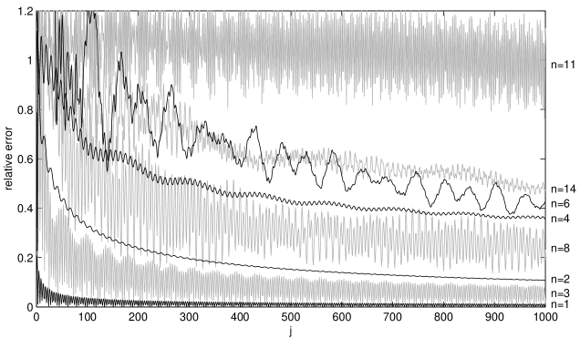
Figure 2: The relative error (24) of various semiclassical traces versus $j$ for $\mu=\omega=\pi(\sqrt{5}-1)$.

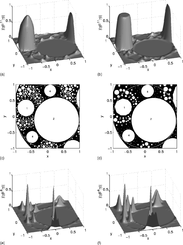
Figure 3: The quantum diagonal matrix element $\langle\gamma|\hat{F}^{n}|\gamma\rangle$ when $j=300$ using the stereographic projection (25), and with (a) $n=11$, $\mu=\omega$, (b) $n=11$, $\mu=\mu_{1}\approx\omega+0.06556$, (e) $n=6$, $\mu=\omega$, and (f) $n=6$, $\mu=\mu_{1}$. The stereographic projection of the classical phase space when (c) $\mu=\omega$ and (d) $\mu=\mu_{1}$.

Figure 3(c) shows the corresponding classical phase space. The periodic points of period 1, 2 and 4 are labeled and the circle $J_{1}=0$ is shown in gray. One can see that an overwhelming contribution to the trace (V) in the form of a large hump is produced by the presence of a classical period-1 orbit. However at $j=300$ the hump does not take the form of a sharp Gaussian peak and is instead quite wide.

Complete failure of the semiclassical trace formula occurs when $\sin S(\bm{\rho})=0$. If this happens in the classical map the local rotation about the stable periodic point $\rho$, given by $2S(\bm{\rho})$, becomes a multiple of $2\pi$. In our case this occurs when $\mu=\mu_{1}\approx\omega+0.06556$ where $\mu_{1}$ is defined via

$$1+2\cos\textstyle\frac{10}{11}\pi=\cos\omega+\cos\omega\cos\mu_{1}+\cos\mu_{1}.$$

The two period-1 orbits now have the action $S\text{ mod }2\pi=5\pi/11$. In more generic systems a period-11 orbit would bifurcate from each period-1 orbit at this point. However no such bifurcation occurs in our mapping. Instead the circular resonance enclosing each of the period-1 orbits takes the form of an 11 sided polygon (Figure 3(d)). Every point inside this polygon rotates $10\pi/11$ radians about the period-1 orbit at each iteration of the mapping, and hence, is a period-11 orbit. The contribution to the semiclassical trace in these special cases is

$$(\,\text{tr}\,\hat{F}^{n})_{sc}=(2j+1)\sum_{\bm{\rho}}\frac{A(\rho)}{4\pi}$$

where $A(\rho)$ is the area on the unit sphere covered by the polygon. In our case we have a regular polygon with area

$$A=2\pi-2n\arcsin\left(\sqrt{1-{J_{1}}^{2}}\sin(\pi/n)\right)$$

where $n=11$ and the period-1 orbit is located at $(J_{1},J_{2},J_{3})$ with

$$J_{1}=\pm\cos(\omega/2)/\sqrt{1+\sin^{2}(\omega/2)\cot^{2}(\mu_{1}/2)}.$$

In Figure 4 we have plotted the semiclassical and quantum traces for this case. The semiclassical displays a good first-order approximation to the quantum. Note that in the limit $j\rightarrow\infty$ the trace is infinite, whereas for $\mu=\mu_{1}\pm\epsilon$ ($\epsilon>0$) the trace limits to a large but finite number. The semiclassical trace is this limit in the latter case. Consequently, when $\epsilon$ becomes small (but still nonzero), the semiclassical trace (21) will be an extremely poor approximate for the quantum, since $j$ needs to be ever larger before the quantum trace reaches its semiclassical limit. Hence the poor convergence in Figure 2 when $n=11$ is explained.

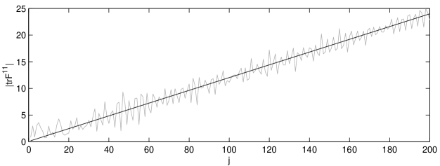
Figure 4: The semiclassical (black) and quantum (gray) trace $\,\text{tr}\,\hat{F}^{11}$ when $\mu=\mu_{1}$.

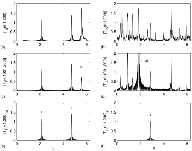
Figure 5: The quantum Fourier transforms $T_{n}(\theta;j_{0},200)$ when (a) $n=6$, $j_{0}=1$, (b) $n=25$, $j_{0}=1$, (c) $n=6$, $j_{0}=1001$, and (d) $n=25$, $j_{0}=1001$. The semiclassical transforms when (e) $n=6$ and (f) $n=25$.

Another test of the semiclassical traces is to consider the quantum Fourier transforms

$$T_{n}(\theta;j_{0},N)=\frac{1}{N}\sum_{j=j_{0}}^{j_{0}+N}e^{-ij\theta}\,\text{tr}\,\hat{F}^{n}$$ (26)

which exhibit peaks at $\theta=2S(\bm{\rho})\text{ mod }2\pi$. In Figures 5(a) and (c) we have plotted the absolute value of the quantum transform $T_{6}$ when $j_{0}=1$ and $j_{0}=1001$, respectively, and $N=200$. Figure 5(e) shows the transform of the semiclassical trace. The peaks have been labeled according to the classical periodic orbit from which they derive. Note that the quantum transforms exhibit a third peak with no semiclassical analogue. This peak illustrates the effect of ‘ghost orbits’ kus2 . It is the result of a residual contribution to the trace, left behind after a pair of period-6 orbits were destroyed when $\mu\approx\omega+0.05318$. In Figure 3(f) we have plotted the quantum diagonal matrix element $\langle\gamma|\hat{F}^{6}|\gamma\rangle$ when $\mu=\mu_{1}\approx\omega+0.06556$ and $j=300$. One finds sharp Gaussian peaks at the location of the classical periodic orbits of periods 1, 2 and 6. The pair of period-6 orbits are marked by $+$’s and $\times$’s in the classical phase space (Figure 3(d)). In spite of there being no classical period-6 orbits when $\mu=\omega$, the quantum diagonal matrix element still displays ghost peaks at their previous locations (Figure 3(e)). These peaks, however, will vanish in the limit $j\rightarrow\infty$ unlike the case of $\mu=\mu_{1}$ where the peaks will instead increase to a height of unity. The exponential decrease in these ghost contributions is also exhibited in the quantum transforms (Figures 5(a) and (c)). Figures 5(b) and (d) show the quantum transform $T_{25}$. The only contribution to the semiclassical trace is from the pair of period-1 orbits (Figure 5(f)). But in the quantum transforms this has been swamped by other contributions. The largest peak in Figure 5(d) is the ghost of a pair of period-25 orbits which were destroyed at $\mu\approx\omega+0.0004288$. This peak has temporarily grown in size after increasing $j$. The other quantum peaks are also believed to be caused by residual quantum effects. However we are currently unable to give an exact reason for their presence.

The quantum transform $T_{25}$ paints a disheartening picture of exponentially proliferating quantum effects not accounted for in the simple semiclassical analysis. In general we found our semiclassical trace $(\,\text{tr}\,\hat{F}^{n})_{sc}$ to be plagued by errors when $n\gtrsim 10$. Although our approximation becomes exact in the limit $j\rightarrow\infty$, and for large $j$ the error is exponentially decreasing, this decay did not occur as quickly as we had hoped. In the next section we find that these inaccuracies make it impossible to extract semiclassical eigenphases from the traces.

VII Numerical investigations of the semiclassical spectrum

Consider the spectral density of the eigenphases

$$\rho(\theta;j) \equiv \sum_{m=0}^{2j}\sum_{k=-\infty}^{\infty}\delta(\theta-\phi_{m}+2k\pi)$$

$$= \frac{1}{2\pi}\sum_{m=0}^{2j}\sum_{n=-\infty}^{\infty}e^{in(\theta-\phi_{m})}$$

$$= \frac{2j+1}{2\pi}+\frac{1}{\pi}\sum_{n=1}^{\infty}\,\text{Re}\,(e^{in\theta}\,\text{tr}\,\hat{F}^{n}).$$

Hence, by rewriting the spectral density in terms of traces of the Floquet operator and using the semiclassical trace formula (21), one may derive a semiclassical spectral density. However, this formula requires traces of the Floquet operator to all powers $n$, which invariably become inaccurate when $n$ is large. Thus, we instead consider the spectral density with limited resolution

$$\rho(\theta;j,N)\equiv\frac{2j+1}{2\pi}+\frac{1}{\pi}\sum_{n=1}^{N}\,\text{Re}\,(e^{in\theta}\,\text{tr}\,\hat{F}^{n})$$

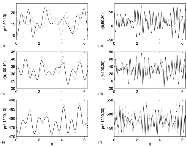
Figure 6: The semiclassical (black) and quantum (gray) spectral density $\rho(\theta;j,N)$ when $N=10$ and (a) $j=50$, (c) $j=100$, (e) $j=1500$, and when $N=30$, (b) $j=50$, (d) $j=100$, (f) $j=1500$.

In figures 6(a), (c) and (e) we plot the semiclassical and quantum (gray) spectral densities when $N=10$ and $j=50$, $100$ and $1500$, respectively. Figures 6(b), (d) and (f) are the same except with $N=30$. The semiclassical approximation is of course most accurate when $j=1500$ and $N=10$. However one needs $N\gg 10$ to resolve the $3001$ eigenphases and even increasing to $N=30$ one finds large discrepancies between the quantum and semiclassical spectral densities.

Another approach kus is to use Newton’s formulae macduffee and rewrite the coefficients of the characteristic polynomial $\det(\hat{F}-z)$ in terms of traces of the Floquet operator. All $2j+1$ eigenphases $\phi_{m}$ can then be extracted via the roots $z_{m}=e^{-i\phi_{m}}$ of the characteristic polynomial. However we still need accurate semiclassical approximates of the trace $\,\text{tr}\,\hat{F}^{n}$ for $1\leq n\leq 2j+1$ (or $1\leq n\leq j+1$ if we enforce ‘selfinversiveness’ on the polynomial i.e. $\det(\hat{F}-z)=z^{2j+1}\det\hat{F}\det(\hat{F}^{\dagger}-z^{-1})$ where $\det\hat{F}=e^{-i\mu j(j+1)}$). The method of harmonic inversion main ; main2 via filter-diagonalization wall ; mandelshtam also proved futile. The problem is not due to the extraction procedure but rather the inaccuracy of our semiclassical trace $(\,\text{tr}\,\hat{F}^{n})_{sc}$ when $n$ becomes large.

Table 2: Semiclassical and quantum eigenphases when $\mu=\omega=\pi(\sqrt{5}-1)$ and $j=100$.

$m$	$n$	$p$	$(\phi_{mnp})_{sc}$	$(\phi)_{qu}$	$\Delta$
0	1	1	1.2064	1.2064	$3\times 10^{-7}$
0	1	$1^{\prime}$	1.2064	1.2064	$4\times 10^{-7}$
1	1	1	4.0846	4.0846	$2\times 10^{-6}$
1	1	$1^{\prime}$	4.0846	4.0846	$2\times 10^{-5}$
2	1	1	0.6797	0.6799	$2\times 10^{-4}$
2	1	$1^{\prime}$	0.6797	0.6800	$3\times 10^{-4}$
6	1	1	5.9093	5.8913	$2\times 10^{-2}$
6	1	$1^{\prime}$	5.9093	5.8533	$6\times 10^{-2}$
0	1	2	2.9306	2.9306	$2\times 10^{-13}$
0	2	2	6.0722	6.0722	$1\times 10^{-13}$
1	1	2	2.2416	2.2416	$1\times 10^{-12}$
1	2	2	5.3832	5.3832	$1\times 10^{-12}$
2	1	2	1.5525	1.5525	$1\times 10^{-12}$
2	2	2	4.6941	4.6941	$1\times 10^{-12}$
57	1	2	1.3544	1.3545	$1\times 10^{-4}$
57	2	2	4.4960	4.4958	$2\times 10^{-4}$
58	1	2	0.6654	0.6657	$3\times 10^{-4}$
58	2	2	3.8070	3.8006	$6\times 10^{-3}$
59	1	2	6.2595	6.2590	$5\times 10^{-4}$
59	2	2	3.1179	3.1340	$2\times 10^{-2}$
0	2	4	5.7403	5.7420	$2\times 10^{-3}$
0	4	4	2.5987	2.6007	$2\times 10^{-3}$
1	4	4	5.6515	5.6454	$6\times 10^{-3}$

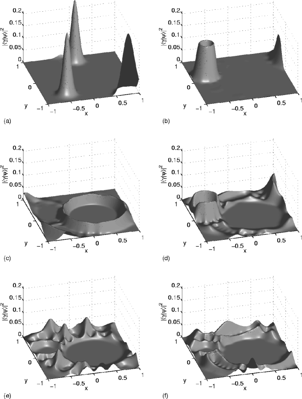
Figure 7: The Husimi functions of selected eigenstates when $\mu=\omega=\pi(\sqrt{5}-1)$ and $j=100$. (a) ($m$,$n$,$p$)=(0,2,4), (b) (2,1,1), (c) (57,1,2), (d) (6,1,$1^{\prime}$), (e) and (f) no association to a periodic orbit.

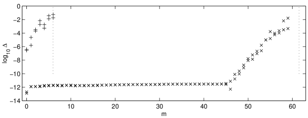
Figure 8: The logarithm of the error in the semiclassical eigenphases versus $m$ for $p=1$ ($+$) and $p=2$ ($\times$).

Our semiclassical eigenphases (22), however, were found to provide good estimates of the quantum eigenphases. Some of the eigenphases for $j=100$ are tabulated in Table 2. The quantum eigenphases $(\phi)_{qu}$ were calculated in the usual manner by diagonalizing the Floquet operator. The Husimi function $|\langle\gamma|\psi\rangle|^{2}$ of each eigenstate was then plotted in phase space to locate the periodic orbit from which it derives. Approximately 142 of the 201 quantum eigenphases could be classified as corresponding to a particular periodic orbit (120 for the period-2 orbit, 14 for the period-1 pair, and 8 for the period-4 orbit).

In Figure 7 we have plotted the Husimi functions of selected eigenstates (refer to Figure 3(c) for the classical phase space). One of the four different ground states associated with the period-4 orbit is plotted in Figure 7(a). The Husimi functions of the three other ground states are very similar to this one. In the limit $j\rightarrow\infty$, each of these states will be in the form of a 4-fold ‘cat state’

$$\textstyle\frac{1}{2}e^{ik\pi/2}|\rho_{1}\rangle+\frac{1}{2}e^{il\pi/2}|\rho_{2}\rangle+\frac{1}{2}e^{im\pi/2}|\rho_{3}\rangle+\frac{1}{2}e^{in\pi/2}|\rho_{4}\rangle$$ (27)

where $k$, $l$, $m$ and $n$ are integers, and $|\rho_{k}\rangle$ is a coherent state centered at the $k$-th iterate of the classical period-4 orbit. Hence, linear combinations of the four ground states with appropriate prefactors of the form $e^{ik\pi/2}/2$, will produce localized states on only one of the four points of the classical orbit.

In Figure 7(b) we have plotted an eigenstate associated with the pair of period-1 orbits. This state is of higher order ($m=2$) and forms rings around the two classical fixed points. The period-1 orbits have degenerate actions (mod $2\pi$), and hence, their semiclassical eigenphases are equal. We have primed the second of each quantum number $p=1$ in Table 2 to emphasize this degeneracy. Note that the quantum eigenphases, however, are unequal. A small splitting allows ‘quantum tunnelling’ dyrting between the period-1 orbits. If we denote the two ground eigenstates by $|011\rangle$ and $|011^{\prime}\rangle$, then the state $|011\rangle+|011^{\prime}\rangle$ will be localized on one of the period-1 orbits, while the state $|011\rangle-|011^{\prime}\rangle$ will be localized on the other. Only after $\pi/|(\phi_{011})_{qu}-(\phi_{011^{\prime}})_{qu}|=3.05\times 10^{7}$ iterations of the quantum mapping, will each of these states have completely tunnelled their way across to each others period-1 point.

In Figure 7(c) we have plotted an eigenstate associated with the period-2 orbit. This is another high-order eigenstate ($m=57$), and despite the large value of $m$, it is immediately recognizable as being derived from the period-2 orbit. An example of when our association becomes questionable is given in Figure 7(d). We have classified this eigenstate as being derived from the period-1 pair. Figures 7(e) and (f) show examples of eigenstates which could not be classified as corresponding to a particular periodic orbit. Our semiclassical analysis affords no description of these eigenstates.

The logarithm of the error in the semiclassical eigenphases

$$\Delta\equiv|(\phi_{mnp})_{sc}-(\phi)_{qu}|$$

versus $m$ is plotted in Figure 8 for the period-1 ($+$) and period-2 ($\times$) orbits. This error decreases exponentially for decreasing $m$. The leveling out for $m\leq 46$ in the period-2 case is due to numerical error attributed to the use of double precision arithmetic. The dotted lines are our estimates for the maximum value of $m$ (23) for which the semiclassical eigenphases will approximate a quantum eigenphase. In the period-1 case $M=5.98$, whilst in the period-2 case $M=61.5$. In both cases our estimates give reasonable approximations.

VIII Conclusion

As a first attempt at applying Gutzwiller’s method of periodic orbit quantization to the mapping under consideration we have had some success. However we have also met great difficulties. We have found that our semiclassical approximation for the trace $\,\text{tr}\,\hat{F}^{n}$ accumulates large errors upon increasing $n$. These errors decay for large $j$, however not at a rate rapid enough for resolution of the semiclassical spectrum. The errors were caused by an exponential proliferation of quantum effects, including ghosts, which were not accounted for in the simple semiclassical analysis. Despite this, our semiclassical eigenphase formula gave an accurate approximation to the quantum eigenphases associated with each periodic orbit. However, this accuracy is hardly surprising given the simplicity of our mapping in the neighborhoods of stable periodic orbits. The global dynamics is of more interest being of high complexity, similar to that of chaotic motion. The semiclassical analysis, however, could not describe eigenstates with support in these parts of the phase space.

The accuracy of our semiclassical trace formula may be increased in three different ways:

1. By including high-order terms in our approximation of the quantum matrix element (11). These terms would need to be included if one were to study the semiclassical role of the unstable set.

2. By including contributions from all saddle points of the integral (19). That is, include the exponentially small terms such as those from ghosts.

3. By including high-order terms along with the first-order approximation (20) for the integral (19). These terms would enhance the accuracy of our trace formula when the action $S$ becomes close to a multiple of $\pi$.

However one must remember that, in general, an asymptotic series is expected to be divergent, and hence, including more terms may prove detrimental if $j$ is not further increased.

The usefulness of Gutzwiller’s method of periodic orbit quantization is debatable. There is no doubt that the theoretical insights offered are second to none. However the practicality of applying such a theory to accurately calculate the eigenphases, or even the traces themselves, is extremely limited. One must always keep in mind that the semiclassical analysis is only valid in the limit $j\rightarrow\infty$. How large $j$ needs to be, before the theory becomes an accurate one, will depend on the specific nature of each particular system. In our case, Gutzwiller’s method has proven inadequate. This failure may be related to the particular dynamical nature of our mapping, which is of extreme ellipticity rather than the preferred hyperbolicity. However we believe that the problems encountered in this study will, in general, reappear in other studies whenever large powers of the Floquet operator are considered. The theory is too simplistic to describe the global complexity encountered in most chaotic systems. Only when $j$ is made large enough, such that some eigenstates will be dominated by the behavior in the immediate vicinity of a periodic orbit, will the theory produce accurate results. This view may be a depressing one, however it is hardly surprising given the particular nature of the Gutzwiller’s approach.

In conclusion, we are left with yet another, albeit cute, example of periodic orbit quantization in an ever expanding sea of literature on the subject. However we hope that our contribution is judged favorably, being qualitatively different from the much explored hyperbolic periodic orbit quantization.

Appendix A Asymptotics of ${\,}_{2}F_{1}(-j,1;j+1;z)$

The hypergeometric function under consideration is first replaced by another using a recurrence relation

$${\,}_{2}F_{1}\Big{(}-j,1;j+1;z\Big{)}=\frac{1}{2}+\frac{1-z}{2}{\,}_{2}F_{1}\Big{(}1-j,1;j+1;z\Big{)}.$$ (28)

This new hypergeometric function can be represented by the integral

$${\,}_{2}F_{1}\Big{(}1-j,1;j+1;z\Big{)}=j\int_{0}^{1}[(1-t)(1-zt)]^{j-1}dt.$$ (29)

When $|z|<1$ a complete asymptotic expansion can be found with the help of a quadratic transformation

$${\,}_{2}F_{1}\Big{(}1-j,1;j+1;z\Big{)} = \frac{1}{1+z}{\,}_{2}F_{1}\Bigg{(}{\textstyle\frac{1}{2}},1;j+1;\frac{4z}{(1+z)^{2}}\Bigg{)}$$ (30)

$$= \frac{1}{1+z}\sum_{m=0}^{n-1}\frac{\Gamma(m+1/2)j!}{\sqrt{\pi}(j+m)!}\left(\frac{4z}{(1+z)^{2}}\right)^{m}+O(j^{-n}).$$ (31)

Taking the limit $n\rightarrow\infty$ the series only converges when $|4z/(1+z)^{2}|\leq 1$, however we still believe it gives a valid asymptotic expansion of (29) if $|z|<1$. This is supported by considering a path of steepest descent in the integral. Letting

$$f(t)=(1-t)(1-zt)$$

we see that an asymptotic expansion of (29) will involve a contribution from the endpoint $t=0$ where $f(t)=1$, and perhaps a contribution from the saddle point $t=1/2(1+1/z)$ where $f^{\prime}(t)=0$. Letting $t=x+iy$, the path of steepest descent from $t=0$ is given implicitly by $\,\text{Im}\,(f(x+iy))=0$. When $|z|<1$ this path is

$$y(x)=\frac{-1}{2\,\text{Im}\,z}\left(1+\,\text{Re}\,z-2x-\sqrt{(1+\,\text{Re}\,z-2x)^{2}+4(1-|z|^{2})x(1-x)}\right)$$

which connects $t=0$ to the other endpoint $t=1$ where $f(t)=0$. Along the contour $f(t)$ is monotonic, and hence, the expansion depends only on the local behaviour near $t=0$. On deriving the first terms in the expansion one finds agreement with (31).

When $|z|>1$ the path of steepest descent from $t=0$ does not pass through $t=1$. It does, however, pass through the other zero at $t=1/z$. To investigate this case we start by rewriting (29) as

$${\,}_{2}F_{1}\Big{(}1-j,1;j+1;z\Big{)} = j\int_{0}^{1/z}[(1-t)(1-zt)]^{j-1}dt+j\int_{1/z}^{1}[(1-t)(1-zt)]^{j-1}dt$$

$$= \frac{j}{z}\int_{0}^{1}[(1-s)(1-s/z)]^{j-1}ds+j(-z)^{-j}(1-z)^{2j-1}\int_{0}^{1}[s(1-s)]^{j-1}ds$$

where we have substituted $t=s/z$ in the first integral and $t=1/z+s(1-1/z)$ in the second ($s$ real). The contour in the second integral takes a path of steepest ascent from $t=1/z$ to the saddle point and then of steepest descent to $t=1$. This integral can be evaluated explicitly, giving an exact contribution from the saddle point. The contour in the first integral is not of steepest descent but now this integral takes the form of (29). We have in fact rederived the linear transformation

$${\,}_{2}F_{1}\Big{(}1-j,1;j+1;z\Big{)}=\frac{1}{z}{\,}_{2}F_{1}\Big{(}1-j,1;j+1;1/z\Big{)}+2\frac{(j!)^{2}}{(2j)!}(-z)^{-j}(1-z)^{2j-1}.$$ (32)

The asymptotic expansion of (29) when $|z|>1$ can now be found by using (31).

In the case $|z|=1$ ($z\neq-1$), the path of steepest descent is a straight line from $t=0$ to the saddle point and then to $t=1$. Hence we rewrite (29) as

$${\,}_{2}F_{1}\Big{(}1-j,1;j+1;z\Big{)} = j\int_{0}^{\frac{1}{2}(1+\frac{1}{z})}[(1-t)(1-zt)]^{j-1}dt+j\int_{\frac{1}{2}(1+\frac{1}{z})}^{1}[(1-t)(1-zt)]^{j-1}dt$$

$$= j(1+1/z)\int_{0}^{\frac{1}{2}}[1-4\cos^{2}(\theta/2)s(1-s)]^{j-1}ds+\frac{(j!)^{2}}{(2j)!}(-z)^{-j}(1-z)^{2j-1}$$

where $z=e^{i\theta}$ and we have substituted $t=s(1+1/z)$ in the first integral and evaluated the second. When $z\neq-1$ the first integral takes its maximum at the endpoint $s=0$. Again, the contribution from this point is (31). There is also a contribution from the endpoint $s=1/2$. This contribution is exponentially smaller, being $O(j^{-n})$ for all $n$, and will be ignored. If, however, $j$ is not large enough the resulting expansion will become inaccurate when $z$ is close to $-1$. Hence we take (31) with the result of second integral as our asymptotic expansion in this case.

Summarizing the above results, when $z\neq-1$ the asymptotic expansion of our original hypergeometric function is

$${\,}_{2}F_{1}\Big{(}-j,1;j+1;z\Big{)} = \frac{1}{2}\Big{[}1-\,\mbox{sgn}\,(1-|z|)\Big{]}\frac{(j!)^{2}}{(2j)!}\Bigg{[}\frac{(1-z)^{2}}{-z}\Bigg{]}^{j}+\frac{1}{2}$$ (33)

$$\quad+\,\,\frac{1}{2}\frac{1-z}{1+z}\sum_{m=0}^{n-1}\frac{\Gamma(m+1/2)j!}{\sqrt{\pi}(j+m)!}\left(\frac{4z}{(1+z)^{2}}\right)^{m}+O(j^{-n})$$

and when $z=-1$ we have the exact result from (32)

$${\,}_{2}F_{1}\Big{(}-j,1;j+1;-1\Big{)}=\frac{(j!)^{2}}{(2j)!}2^{2j-1}+\frac{1}{2}.$$ (34)

We have tested these asymptotics numerically and found good agreement. However convergence is weak near $z=-1$.

Appendix B A multiple integral

Consider the relation

$$I_{n}(a_{1}^{\phantom{*}},\dots,a_{n}^{\phantom{*}})\equiv\int\prod_{k=1}^{n}d^{2}z_{k}^{\phantom{*}}\,\,e^{a_{k}^{\phantom{*}}z_{k+1}^{*}z_{k}^{\phantom{*}}-z_{k}^{*}z_{k}^{\phantom{*}}}=\frac{\pi^{n}}{1-a_{1}^{\phantom{*}}\dots a_{n}^{\phantom{*}}}$$

where we have assumed the integral is convergent, $z=x+iy$, $d^{2}z=dxdy$ and the subscript $n+1\equiv 1$. The proof is relatively simple and is achieved through induction. When $n=1$ the integral is trivial. We now assume the equality holds for $n=m$ and consider the case $n=m+1$

$$I_{m+1}(a_{1}^{\phantom{*}},\dots,a_{m+1}^{\phantom{*}}) = \int d^{2}z_{1}^{\phantom{*}}\dots d^{2}z_{m+1}^{\phantom{*}}\,\,e^{a_{1}^{\phantom{*}}z_{2}^{*}z_{1}^{\phantom{*}}+\dots+a_{m}^{\phantom{*}}z_{m+1}^{*}z_{m}^{\phantom{*}}+a_{m+1}^{\phantom{*}}z_{1}^{*}z_{m+1}^{\phantom{*}}-z_{1}^{*}z_{1}^{\phantom{*}}-\dots-z_{m+1}^{*}z_{m+1}^{\phantom{*}}}$$

$$= \pi\int d^{2}z_{1}^{\phantom{*}}\dots d^{2}z_{m}^{\phantom{*}}\,\,e^{a_{1}^{\phantom{*}}z_{2}^{*}z_{1}^{\phantom{*}}+\dots+a_{m-1}^{\phantom{*}}z_{m}^{*}z_{m-1}^{\phantom{*}}+a_{m}^{\phantom{*}}a_{m+1}^{\phantom{*}}z_{1}^{*}z_{m}^{\phantom{*}}-z_{1}^{*}z_{1}^{\phantom{*}}-\dots-z_{m}^{*}z_{m}^{\phantom{*}}}$$

$$= \pi I_{m}(a_{1}^{\phantom{*}},\dots,a_{m-1}^{\phantom{*}},a_{m}^{\phantom{*}}a_{m+1}^{\phantom{*}})$$

$$= \frac{\pi^{m+1}}{1-a_{1}^{\phantom{*}}\dots a_{m}^{\phantom{*}}a_{m+1}^{\phantom{*}}}$$

Hence the equality is true for all $n$. By making appropriate substitutions for $a_{k}$ and $z_{k}$ the multiple integral (20) is solved.

References

- (1) M.C. Gutzwiller, J. Math. Phys. 8, 1979 (1967); 10, 1004 (1969); 11, 1791 (1970); 12, 343 (1971).
- (2) M.C. Gutzwiller, Chaos in Classical and Quantum Mechanics (Springer-Verlag, New York, 1990).
- (3) A. Einstein, Verhandl. Deut. Phys. Ges. 19, 82 (1917); L. Brillouin, J. Phys. Radium 7, 353 (1926); J.B. Keller, Ann. Phys. 4, 180 (1958).
- (4) M.V. Berry and M. Tabor, Proc. R. Soc. London A 349, 101 (1976); J. Phys. A 10, 371 (1977).
- (5) A.M. Ozorio de Almeida, Hamiltonian Systems: Chaos and Quantization (Cambridge University Press, Cambridge, 1988).
- (6) S. Tomsovic, M. Grinberg and D. Ullmo, Phys. Rev. Lett. 75, 4346 (1995); D. Ullmo, M. Grinberg and S. Tomsovic, Phys. Rev. E 54, 136 (1996).
- (7) M. Sieber, J. Phys. A 30, 4563 (1997).
- (8) H. Schomerus and F. Haake, Phys. Rev. Lett. 79, 1022 (1997).
- (9) J. Main and G. Wunner, Phys. Rev. Lett. 82, 3038 (1999).
- (10) F. Haake, Quantum Signatures of Chaos (Springer-Verlag, Berlin, 1991).
- (11) M. Tabor, Physica D 6, 195 (1983).
- (12) G. Junker and H. Leschke, Physica D 56, 135 (1992).
- (13) A. Lakshminarayan, Paramana J. Phys. 48, 517 (1997).
- (14) J.P. Keating, Nonlinearity 4, 309 (1991).
- (15) P.A. Boasman and J.P. Keating, Proc. R. Soc. London A 449, 629 (1995).
- (16) A. Lakshminarayan, Phys. Lett. A 192, 345 (1994).
- (17) M.M. Sano, J. Phys. A 29, 6087 (1996).
- (18) B. Eckhardt and F. Haake, J. Phys. A 27, 4449 (1994).
- (19) M. Saraceno and A. Voros, Physica D 79, 206 (1994).
- (20) A. Lakshminarayan, Ann. Phys. 239, 272 (1995).
- (21) F. Toscano, R.O. Vallejos and M. Saraceno, Nonlinearity 10, 965 (1997).
- (22) G. Tanner, J. Phys. A 32, 5071 (1999).
- (23) M. Kuś, F. Haake and B. Eckhardt, Z. Phys. B 92, 221 (1993).
- (24) M. Kuś, F. Haake and D. Delande, Phys. Rev. Lett. 71, 2167 (1993).
- (25) R. Scharf and B. Sundaram, Phys. Rev. E 49, R4767 (1994).
- (26) B. Sundaram and R. Scharf, Physica D 83, 257 (1995).
- (27) R. Scharf and B. Sundaram, Phys. Rev. Lett. 77, 263 (1996).
- (28) K. Saito and T. Nagao, J. Phys. Soc. Japan 68, 1131 (1999).
- (29) E.B. Bogomolny, Nonlinearity 5, 805 (1992).
- (30) A.J. Scott, C.A. Holmes and G.J. Milburn, Physica D 155, 34 (2001).
- (31) O. Bohigas, M.J. Giannoni and C. Schmit, Phys. Rev. Lett. 52, 1 (1984).
- (32) A. Perelomov, Generalized Coherent States and Their Applications (Springer-Verlag, Berlin, 1986).
- (33) J. Janszky, P. Domokos and P. Adam, Phys. Rev. A 48, 2213 (1993).
- (34) C.C. MacDuffee, Theory of Equations (Wiley, New York, 1954).
- (35) J. Main, V.A. Mandelshtam and H.S. Taylor, Nonlinearity 11, 1015 (1998).
- (36) J. Main, Phys. Rep. 316, 233 (1999).
- (37) M.R. Wall and D. Neuhauser, J. Chem. Phys. 102, 8011 (1995).
- (38) V.A. Mandelshtam and H.S. Taylor, Phys. Rev. Lett. 78, 3274 (1997); J. Chem. Phys. 107, 6756 (1997).
- (39) S. Dyrting, G.J. Milburn and C.A. Holmes, Phys. Rev. E 48, 969 (1993).
- (40) A. Erdélyi et al., Higher Transcendental Functions: Volume I (McGraw-Hill, New York, 1953).