Resonance Effects in Topological Discrete sine-Gordon System

Abstract

We consider kink-antikink collisions in the TDSG system introduced by Speight and Ward in 1994. We find that the TDSG kink supports extra internal modes of vibration and this results in resonance effects of the kind seen for the continuum $\phi^{4}$ system.

1. Introduction

Nonlinear systems which have soliton solutions have played an increasingly important role in physics. One such area in physics is condensed matter theory where the soliton has been used to model crystal discolations, charge density waves, magnetic domain walls, etc [1]. In many cases it has been necessary to model interactions of the soliton with other objects such as impurities, defects, phonons, antisolitons, or other solitons. In (1+1)-dimensional field theories, these interactions have sometimes been quite spectacular, particularly if the 1-dimensional soliton, or the kink, supports extra modes of vibration. Such a mode can be excited during an interaction and this leads to a “resonance effect” [2]. This effect has been seen in both continuous and discrete systems [1-8]. These resonance effects give rise to “windows” in the space of impact velocity, i.e. there are certain intervals of velocities in this space for which the kinks form a bound state (a bion) and others for which the kinks scatter off each other.

This paper deals with kink-antikink collisions in the topological discrete sine-Gordon system (TDSG) introduced by Speight and Ward in 1994. This system is particularly interesting since it is a discrete system but with many of the features of the continuum sine-Gordon. In particular, it maintains the Bogomoln’yi bound. The resulting Bogomoln’yi equation is a first-order difference equation which can be easily solved. The solution is analogous to the well-known continuum sine-Gordon static kink solution. Moreover, as we show in section 4, the TDSG kink supports an internal shape mode.

The paper is divided into 5 sections. Section 2 contains a brief summary of kink dynamics in the TDSG system [10], [14]. In section 3 we consider the kink-antikink collisions in the TDSG. In section 4 we show that TDSG kink supports an internal mode of vibration and section 5 contains some concluding remarks.

2. Kink dynamics in TDSG

The TDSG system is defined by the Lagrangian density

$$\mathcal{L}=\frac{h}{4}\sum_{n\in{Z}}(\dot{\psi_{n}}^{2}-(D_{n}^{2}+F_{n}^{2})),$$ (1)

where the kinetic energy is $E_{K}=\frac{h}{4}\sum\dot{\psi}_{n}^{2}$ and the potential energy is $E_{P}=\frac{h}{4}\sum(D_{n}^{2}+F_{n}^{2})$.

The quantities $D_{n}$ and $F_{n}$ are given by

$$D_{n}=\frac{2}{h}\sin\frac{1}{2}(\psi_{n+1}-\psi_{n})\quad\textnormal{and}\quad F_{n}=\sin\frac{1}{2}(\psi_{n+1}+\psi_{n}),$$ (2)

giving

$$E_{P}=\frac{h}{4}\sum\frac{4}{h^{2}}\sin^{2}\frac{1}{2}(\psi_{n+1}-\psi_{n})+\sin^{2}\frac{1}{2}(\psi_{n+1}+\psi_{n}).$$ (3)

$\psi_{n}=\psi(x)$ at the $n^{th}$ lattice site and $\psi_{n+1}=\psi(x+h)$, where $h$ is the lattice spacing. The first term in equation (3) represents an attractive force analogous to the Hooke force. The second term is the substrate potential, found by taking an average of the potential of the two nearest neighbours.

In the continuum limit, as $h\rightarrow 0$, $D_{n}\rightarrow\psi_{x}$, and $F_{n}\rightarrow\sin\psi$, and one recovers the standard expression of the continuum potential

$$E^{cont}_{P}(\psi)=\frac{1}{4}\int_{-\infty}^{\infty}(\psi_{x}^{2}+\sin^{2}\psi)\,dx.$$ (4)

The key feature of this model is the choice of the derivative on the lattice. This choice is motivated by the Bogomol’nyi argument of the continuum system. Rather than choose the standard forward difference, Speight and Ward choose,

$$-\frac{\cos\psi_{n+1}-\cos\psi_{n}}{h}=D_{n}F_{n},$$ (5)

with the kink boundary conditions

$$\lim_{n\rightarrow-\infty}\psi_{n}=0\quad\textnormal{and}\quad\lim_{n\rightarrow\infty}\psi_{n}=\pi.$$

This leads to the following discrete Bogomol’nyi argument

$$0 \leq\frac{h}{4}\sum_{n\in Z}(D_{n}-F_{n})^{2}$$ (6)

$$=E_{P}+\frac{1}{2}\sum_{n\in Z}(\cos\psi_{n+1}-\cos\psi_{n})$$ (7)

$$=E_{P}-1,$$ (8)

so $E_{P}\geq 1$, with equality if $D_{n}=F_{n}$, i.e. if

$$\qquad\qquad\frac{2}{h}\sin\frac{1}{2}(\psi_{n+1}-\psi_{n})\quad =\sin\frac{1}{2}(\psi_{n+1}+\psi_{n})$$ (9)

$$\textnormal{or,}\quad\quad\psi_{n} =2\tan^{-1}\exp{a(nh-b)}.$$ (10)

The constant $a=h^{-1}\ln[\frac{2+h}{2-h}]$ is the kink’s slope and $b\in R$ is the position. Equation (10) is the static kink solution. So the moduli space of static solutions for the TDSG is isomorphic to $\mathbb{R}$ rather than $\mathbb{Z}$, which is what one usually expects for a discrete system. Moreover, $E_{P}$ is independent of $b$ suggesting that the model has no Peierls-Nabarro barrier. This means that the kink can move along the lattice arbitrarily slowly without getting pinned.

The Euler-Lagrange equation gives the following equation of motion,

$$\ddot{\psi_{n}}=\frac{4-h^{2}}{4h^{2}}\cos\psi_{n}(\sin\psi_{n+1}+\sin\psi_{n-1})-\frac{4+h^{2}}{4h^{2}}\sin\psi_{n}(\cos\psi_{n+1}+\cos\psi_{n-1}).$$ (11)

Equation (11) can then be used to study the behaviour of a moving kink. Speight and Ward have solved (11) using a 4th-order Runge-Kutta scheme. Their initial condition was a static kink Galilean boosted to a velocity $v$. Their results show that for small initial velocities the kink wobbles with a period $h/v$ as it moves along the lattice. This is a purely dynamical effect since there is no Peierls-Nabarro barrier.

For fast moving kinks it is found that the kink radiates as it moves along the lattice. This is observed through a gradual decrease in the kink velocity. But it is found that there is certain velocity threshold below which the radiation from the kink is significantly reduced.

The existence of such a velocity threshold can be understood by considering the linearised equation of motion [10].

$$\ddot{\psi_{n}}=\frac{4-h^{2}}{4h^{2}}(\psi_{n+1}+\psi_{n-1})-\frac{4+h^{2}}{2h^{2}}\psi_{n}.$$ (12)

Equation (12) can be used to derive a dispersion relation for small amplitude travelling waves, given by

$$\omega^{2}=\frac{4+h^{2}}{2h^{2}}-\frac{4-h^{2}}{2h^{2}}\cos kh,$$ (13)

where $k$ is the wavenumber. Since $0<h<2$, we have $1<\omega<2/h$. The case $\omega=1$ corresponds to the threshold velocity. The frequency at which the kink hits the lattice sites is $v/h$ per unit time. So provided $v\geq h/2\pi$, the kink will radiate (at $\omega=2\pi v/h$). But if $v<h/2\pi$ then $\omega<1$ and the kink does not radiate. Hence there is a ”preferred” velocity for the kink. Since this velocity depends only on $h$, it can be regarded as a feature of the lattice.

The choice of the functions $D_{n}$ and $F_{n}$ is not unique. For instance, $D_{n}$ could be multiplied by a function $f(x,h)$ and $F_{n}$ by $f(x,h)^{-1}$ and the product is independent of $f$ so one would still have a topologically stable kink solution. The only condition on $f(x,h)$ is that $\lim_{h\rightarrow 0}f=1$. Similarly there is freedom in the choice of $\ddot{\psi}$. Zakrzewski [14] has investigated the effects on the kink motion when this choice is exploited.

The $\ddot{\psi}$ in (11) is replaced by

$$\ddot{\psi}\rightarrow\frac{\ddot{\psi}}{1+\alpha\dot{\psi}^{2}}$$ (14)

where $\alpha=\alpha(h)$ and $\alpha(0)=1$. The equation of motion (11) is now changed to

$$\frac{\ddot{\psi}_{n}}{(1+\alpha\dot{\psi_{n}}^{2})}=\frac{f^{2}}{h^{2}}(\sin(\psi_{n+1}-\psi_{n})-\sin(\psi_{n}-\psi_{n-1}))-\frac{1}{4f^{2}}(\sin(\psi_{n+1}+\psi_{n})+\sin(\psi_{n}+\psi_{n-1})).$$ (15)

The choices of $f$ and $\alpha$ are motivated by the fact that equation (15) still needs to admit the Galilean boosted sine-Gordon kink solution. One choice is the following

$$f^{2}=\frac{\frac{v_{1}^{2}}{1-v_{1}^{2}}+\sqrt{\left(\frac{v_{1}^{2}}{1-v_{1}^{2}}\right)^{2}+\frac{4\sinh^{2}2\beta}{h^{2}}}}{\frac{8\sinh^{2}\beta}{h^{2}}}$$ (16)

where $\beta=h/2\sqrt{1-v_{1}^{2}}$, and

$$\alpha(h)=\frac{1-v_{1}^{2}}{v_{1}^{2}}\sinh^{2}(2\beta).$$ (17)

Numerical simulations of (15) using a 4th-order Runge-Kutta method has shown that the kink propagates without emitting any radiation if the initial velocity of the kink is chosen to be the velocity $v_{1}$ used in the expression of $f^{2}$. For initial velocities $v\leq v_{1}$, there is virtually no emission of radiation so the kink velocity hardly decreases. For $v>v_{1}$, the kink initially propagates at velocity greater than $v_{1}$ but then slows down to a velocity just less than $v_{1}$ after which it’s virtually constant with little emission of radiation. The initial increase in velocity is due to the readjustment of the kink configuration to match the lattice field configuration.

3. Kink-antikink Collisions in the TDSG System

3.1 Preliminaries

In this section we present results of kink-antikink interactions in the Speight-Ward model. The results are obtained by solving (11) with the initial condition corresponding to Galilean boosted static kink and antikink solutions at each end of the lattice grid, i.e.

$$\psi(x,0) =2\tan^{-1}\exp a(x+b)-2\tan^{-1}\exp a(x-b),$$ (18)

$$\dot{\psi}(x,0) =-av(\textnormal{sech}\,a(x+b)+\textnormal{sech}\,a(x-b)).$$ (19)

The boundary condition is taken to be $\psi(x_{min})=\psi(x_{max})=0$, i.e. the ends of the kink and anti-kink are held fixed at all times.

The kink and antikink move towards each other with relative velocity $2v$. Equation (11) is solved using a 4th-order Runge-Kutta algorithm. The programme is run with various lattice spacings $h$. The time step is chosen to be 0.05. This conserves the energy to within 0.05% in a simulation which runs for 1000 units. We use the same time step for all values of $h$.

Our choice of the boundary condition means that any radiation emitted by the kink will reflect off the edges and eventually interact with the kinks. This is easily avoided by making the grid sufficiently large.

As mentioned already, the amount of radiation emitted by the kink depends on the kink velocity and also on the lattice spacing. For large velocities and coarser lattices the amount of radiation is significantly greater. In these cases we have damped the first few lattice sites at each end of the grid. That is, the value of $\dot{\psi}$ at these sites is decreased by a constant amount (10%) for the entire duration of the simulation. The total energy of the system is of course no longer conserved. The energy loss depends on the initial velocity of the kink and on the lattice spacing, but it is usually within 10% of the initial energy, for a simulation running for 1000 units.

3.2 Simulation Results

The simulations showed that the outcome of an interaction depends on the impact velocity of the kinks. The velocity of the kink (or the antikink) is defined to be the rate of change of $X(t)$, where $X(t)$ is the “average” position of the kink (or the antikink). $X(t)$ for the kink is given by

$$X(t)=\frac{\displaystyle\sum_{i=-N}^{0}x_{i}e_{i}}{\displaystyle\sum_{i=-N}^{0}e_{i}}.$$ (20)

Here $e_{i}$ is the total energy of the field and the radiation at the $i^{th}$ lattice site, where $x_{i}=x_{min}+ih$. The quantity $\sum_{-N}^{0}e_{i}$ is the total energy of the field and the radiation for the single kink. We found that for cases when the phonon radiation from the kinks is not significant, $X(t)$ makes a good approximation to the kink position. We define the velocity of the kink to be $\dot{X}(t)$, which is computed using the forward difference, $\dot{X}(t)=\frac{1}{\Delta t}(X(t+\Delta t)-X(t))$.

Since the kink wobbles as it moves along the lattice, $\dot{X}(t)$ is an oscillating function. The period of oscillation is the wobble period, $h/v$, where $v$ is the velocity used in the initial condition (19). This wobble can be understood by considering the geodesic motion on the kink moduli space. This moduli space has a periodic metric [10].

Figure 1 shows various plots of kink velocity against time for kinks with different initial positions. The kinks are on a lattice with $h=1.4$ and the initial velocity of the kink is $v=0.197$. In all cases the average velocity of the kink is significantly decreased. This is due to phonon radiation from the kinks. The plots also show that the kink velocity depends on the initial position of the kink, modulo $nh$, where $n\in\mathbb{Z}$.

The outcome of an interaction has sensitive dependence on the velocity of the kink. In particular, there are three different outcomes:

(a)   If the kink impact velocity is above a certain critical velocity, $v_{c}$, then the kinks simply pass through each other, i.e. there is a smallest number $v_{c}$ such that the outcome of the interaction for all $v\geq v_{c}$ is always a passing through behaviour. The value of $v_{c}$ depends on the lattice spacing and also on $b$. Figure 2 shows the dependence of $v_{c}$ against $h$. The dotted curve represents the quadratic $0.073h^{2}+0.036h$. This curve is an empirical fit to the data points and is not derived from the theory.

The dependence of $v_{c}$ on the position of the kinks is due to dynamical dressing and the kink wobble. For small initial velocities (figure 1), the kink velocity oscillates with a period $(h/v)$. The amplitude of oscillation is of the order of $10^{-2}$. For large velocities, the phonon radiation make the oscillations erratic and also significantly decrease the overall velocity of the kink. The initial velocity also changes due to the readjustment of the kink field to suit the lattice distribution (dynamical dressing). The initial propagating velocity of the kink is not always $v$, the velocity used in expression (19). In some cases it is larger than $v$ and in others it is less than $v$. This change depends on the magnitude of $v$ and on the lattice spacing. The effect can be seen in figure 1.

Figure 1: A plot of the kink velocity against time. The three curves represent velocities of kinks with an initial velocity of 0.197 but starting at different points on the lattice. The solid curve represents a kink with $b=30$, the dashed curve a kink with $b=25$ and the dotted curve is for $b=15$.

Figure 2: A plot of critical velocity against lattice spacing. The crosses represent data points found numerically. The curve represents a theoretical fit of $v_{c}=0.073h^{2}+0.036h$.

For initial kink velocities which give impact velocities below $v_{c}$, we found that the outcome is either (b) a bounce or (c) a trapped breather-like state (a bion). The bounce is essentially a kink-antikink scattering, where the kinks after the first collision pass through each other but fail to escape to infinity. Instead, they travel a small distance and then turn around for another collision. After the second collision the kinks either escape to infinity or turn around again for more collisions. For a 2-bounce event (meaning the kinks pass each other twice) the ultimate outcome of this scattering would be a reflection, and for a 3-bounce a transmission.

The velocities for the bounces occur in small intervals. For velocities outside of these intervals the outcome is always a bound state. This is similar to the results for the $\phi^{4}$ model [4], except in this case the outcome does not depend fractally on the impact velocity. We have only seen 2, 3 and 4-bounce events. But the velocities at which the bounces occur are not easy to find and the intervals are small ($10^{-7}$ for a 4-bounce), so it may be that higher bounce events occur but we have not seen them.

Figure 3 shows an example of the 2-bounce event. In this figure we have plotted the field $\psi(0,t)$ against $t$. $\psi(0,t)$ is the field at the centre of mass of the kink-antikink system.The kinks are on a lattice of unit spacing with an initial separation of 10 units. $v_{c}$ for this combination is found to be 0.100. The kinks bounce for all initial velocities in the range $0.0969\leq v\leq 0.0972$ (2-bounce window).

Figures 4 and 5 show examples of three and four bounce events. In figure 4 the kinks transmit whereas in 5 they reflect off each other. As can be seen from the figure for the 2-bounce case, the kink and antikink collide, pass through each other and travel a small distance before stopping, turning around and travelling in the other direction. The kinks then collide again, pass through each other and this time escape to infinity.

Figure 3: A figure representing the 2-bounce event. The kinks collide and essentially reflect off each other.

Figure 4: A 3-bounce event where the scattering of the kinks results in a transmission.

Figure 5: A plot showing a 4-bounce event.

Figure 6: A plot of $\psi(0,t)$ against time, representing the oscillations at the centre of mass of the bion.

Figure 6 is a graph of $\psi(0,t)$ against $t$ representing the oscillations at the centre of mass of a bion. This is essentially an $n$-bounce event for $n$ very large. The erratic oscillations suggest that the system might be chaotic. The period of oscillations become constant after about 10 cycles and the bion then oscillates for a long time (i.e for hundreds of cycles). We have calculated the maximum Lyapunov exponent of the time series $\psi(0,t)$, using the algorithm of Wolf et al [15]. Its value is approximately 0.18, suggesting that the oscillations are mildly chaotic. In general, a positive maximum Lyapunov exponent is taken as a formal definition of chaos.

The results of the simulation can be understood using the resonance energy exchange mechanism. This requires the TDSG kink to support shape modes. We show next that the TDSG kink does support such a mode. The frequency of this mode is calculated in two ways, by using a collective coordinate approximation and also numerically, by Fourier analysing the deformations of a perturbed static kink. Note that we could also have used a matrix-based approach similar to the one used by Speight in [16], where it was used to calculate the Casimir energy of the kink.

4. Kink internal shape mode

4.1 Collective coordinate approximation

We can obtain a collective coordinate approximation of the TDSG system by treating the scale factor $a$ in the kink as a dynamical variable. This reduces the number of degrees of freedom from infinity to one. The Lagrangian of the reduced system is given by

$$\mathcal{L}=f(a,b)\dot{a}^{2}-g(a,b),$$ (21)

where $f(a,b)$ and $g(a,b)$ are functions given by

$$f(a,b) =\frac{h}{4}\sum_{x}(x-b)^{2}\textnormal{sech}^{2}a(x-b),$$ (22)

$$g(a,b) =\frac{1}{h}\tanh(\frac{1}{2}ah)+\frac{h}{4}\coth(\frac{1}{2}ah).$$ (23)

The corresponding equation of motion is

$$2f\ddot{a}+f^{\prime}\dot{a}^{2}-g^{\prime}=0.$$ (24)

where the prime denotes differentiation with respect to $a$. $g(a,b)$ has a minimum (stable equilibrium) at $a=s:=\frac{2}{h}\tanh^{-1}\frac{h}{2}$. Small amplitude oscillations $a(t)=s+\epsilon(t)$ satisfy the linearised equation,

$$2f(s,b)\ddot{\epsilon}=g^{\prime\prime}(s,b)\epsilon.$$ (25)

Hence the waves oscillate with frequency

$$\nu=\frac{1}{2\pi}\sqrt{\frac{g^{\prime\prime}(s)}{2f(s,b)}}.$$ (26)

$g^{\prime\prime}(s)=(1-\frac{1}{4}h^{2})^{2}$, so the frequency of the shape mode depends on the lattice spacing. For $h=1$, the shape mode frequency is 0.152. Table 1 shows the dependence of frequency on the lattice spacing $h$.

h	frequency
0.1	0.175
0.2	0.175
0.5	0.170
0.8	0.161
0.9	0.157
1.0	0.152
1.2	0.143

As a check on the accuracy of the collective coordinate approach, we have used it to calculate the frequency of the shape mode of the $\phi^{4}$ kink. The value found is $\sqrt{(}1.55)$, which is fairly close to the actual value $\sqrt{(}1.5)$.

4.2 Numerical method

Numerically, the shape mode frequency is obtained by Fourier analysing the deformations of the perturbed static kink. We set the initial condition for equation (11) to be

$$\psi(x,0) =\psi_{K}(x,0)+\epsilon$$ (27)

$$\dot{\psi}(x,0) =0,$$

where $\psi_{K}(x)$ is the static kink solution and $\epsilon$ is the pertubation. The value of $\epsilon$ is chosen to be -0.03. The field $\psi(x,t)$ is sampled at various values of $x$. From this we obtain the variations in the field, $\delta\psi(x,t)=\psi(x,t)-\psi(x,0)$, for each of the sampled values of $x$. $\delta\psi(x,t)$ were then Fourier analysed using the MATLAB FFT routine.

In figure 7 we have plotted the power spectrum for the data sampled at $x=0$ for a kink on an $h=1$ lattice. The power spectrum of the data for other values of $x$ give identical power spectrums.

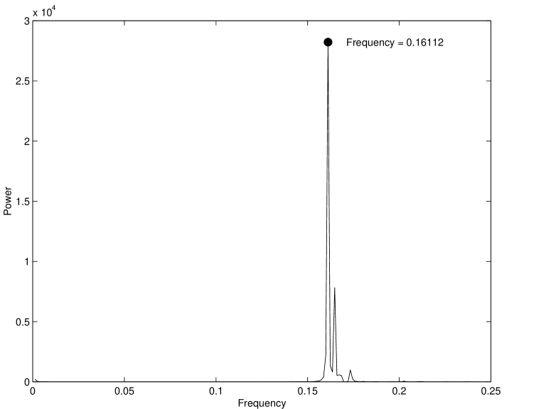
Figure 7: Power spectrum of the fluctuations around a perturbed static kink

Figure 7 was constructed using $N=2^{14}=16384$ data points. Aliasing of the power does not occur since the amplitude at the Nyquist frequency is essentially zero. There is a peak at $\nu=0$ corresponding to the Goldstone mode, and a peak at $\nu=0.161$ corresponding to the shape mode.

This procedure is repeated for other values of $h$. In contrast to the results suggested by the collective coordinate approach, we find that the frequency of the shape mode is more or less independent of $h$. For $0.5\leq h\leq 1.2$, we found $0.158<\nu<0.161$. The value of the frequency (for $h=1$) however is within the range of frequencies found using the collective coordinate method.

In the continuum limit the TDSG shape mode frequency is precisely the quasimode frequency of the continuum sG system found by Rice, $\omega_{R}=0.175$ [12], although it is unlikely that such a quasimode exists [17]

It is interesting to compare the situation with other discrete sine-Gordon systems. The well-known Frenkel-Kontorrova model does not support a kink with an internal shape mode for all values of the discreteness parameters. The sine-Lattice model (s-L) however does support one, as long as the system is only weakly discrete [7]. The shape mode for the s-L system lies just above the lower phonon band suggesting that it is a genuine kink shape mode rather than just a phonon resonance. Moreover, in the continuum limit this shape mode converges to the sine-Gordon quasimode frequency. The existence of a shape mode in a discrete sine-Gordon system depends on the anharmonicity of the potential term.

5. Conclusion

We have found that the kink-antikink interactions in the TDSG system exhibit resonance phenomena similar to those in the continuum $\phi^{4}$ system. These are found to be due to the excitation of an intermal mode of the TDSG kink. A collective coordinate analysis shows that the frequency of this mode depends on the lattice spacing, and in the continuum limit $(h\longrightarrow 0)$ the frequency seems to approach the quasimode frequency predicted by Rice. The recent analysis done in [17] however says that there cannot be a quasimode for the continuum sine-Gordon kink, but they do predict the existence of a quasimode for a lattice sine-Gordon kink. This is not the quasimode we have found, so this is something genuinely new. Further numerical simulations are required to determine what is happening in the limit $h\longrightarrow 0$.

Also, as we have mentioned already, there is a modified TDSG system [14] which admits an exact travelling-kink solution (with a fixed velocity). It would be interesting to perform kink-antikink interactions for this system. Since the expressions we have used to perform the interactions are only an approximation to the equation of motion, it would be interesting to see the difference.

We have also done kink-antikink collision simulations for the TD$\phi^{4}$ system [18]. The results are found to be analoguos to the conventional discrete $\phi^{4}$ system [4], though in the “windows” structure in the space of impact velocity is not a fractal.

Acknowledgements I would like to thank Richard Ward for helpful discussions and EPSRC for a research studentship.

References

- [1] A.R.Bishop and T.Scheider (1983) Solitons and Condensed Matter Physics (Springer-Verlag).
- [2] D.K.Campbell, J.F.Schonfeld and C.A.Wingate (1983). Resonance structure in kink-antikink interactions in theory, Physica 9 D 1-32.
- [3] T.Belova and A.E.Kudryavtsev (1988). Quasiperiodical orbits in the scalar classical field theory, Physica D 32 18.
- [4] P.Anninos, S.Oliveira, and R.A.Matzner (1991). Fractal structure in the scalar model, Phys Rev D 44 1147.
- [5] M.J.Ablowitz, M.D.Kruskal and J.F.Ladik (1979). Solitary wave collisions, Siam J Appl Maths 36 428-437.
- [6] V.A.Gani and A.E.Kudryavtsev (1998). Kink-antikink interactions in the double sine-Gordon equation and the problem of resonance frequencies, cond-mat/9809015.
- [7] Fei Zhang (1997). Kink shape modes and resonant dynamics in sine-lattices, Physica D 110 51-61.
- [8] A.E.Kudryavtsev (1975). Solitonlike solutions for a Higgs scalar field., JETP Lett 22 82-83.
- [9] D.K.Campbell, M.Peyrard and P.Sodano (1986). Kink-antikink interactions in the double sine-Gordon equation, Physica 19 D 165-205.
- [10] J.M.Speight and R.S.Ward (1994). Kink dynamics in a novel discrete sine-Gordon system, Nonlinearity 7 475-484.
- [11] M.Peyrard and D.K.Campbell (1983). Kink-antikink interactions in the parametrically modified sine-Gordon system, Physica 9 D 33-51.
- [12] M.J.Rice (1983). Physical dynamics of solitons, Phys Rev B 28 3587-3589.
- [13] R.Boesch and C.R.Willis (1990). Existence of an internal quasimode for a sine-Gordon soliton, Phys Rev B 42 2290.
- [14] W.J.Zakrzewski (1994). A modified discrete sine-Gordon model, Nonlinearity 8 517-540.
- [15] A.Wolf, J.B.Swift, H.L.Swinney and J.A.Vastano (1985). Determining Lyapunov exponents from a time series, Physica D 16 285-317.
- [16] J.M.Speight (1994). Kink Casimir energy in a lattice sine-Gordon model, Phys Rev D 49 6914-6919.
- [17] Niurka R. Quintero, Angel Sanchez and Franz G. Mertons (2000). Existence of internal modes of sine-Gordon kinks, Phys Rev E 62 R60-R63.
- [18] J.M.Speight (1997). A discrete system without a Peierls-Nabarro barrier, Nonlinearity 10 1615-1625.