Bifurcations in annular electroconvection with an imposed shear

Abstract

We report an experimental study of the primary bifurcation in electrically-driven convection in a freely suspended film. A weakly conducting, submicron thick smectic liquid crystal film was supported by concentric circular electrodes. It electroconvected when a sufficiently large voltage $V$ was applied between its inner and outer edges. The film could sustain rapid flows and yet remain strictly two-dimensional. By rotation of the inner electrode, a circular Couette shear could be independently imposed. The control parameters were a dimensionless number ${\cal R}$, analogous to the Rayleigh number, which is $\propto V^{2}$ and the Reynolds number ${\cal R}e$ of the azimuthal shear flow. The geometrical and material properties of the film were characterized by the radius ratio $\alpha$, and a dimensionless number ${\cal P}$, analogous to the Prandtl number. Using measurements of current-voltage characteristics of a large number of films, we examined the onset of electroconvection over a broad range of $\alpha$, ${\cal P}$ and ${\cal R}e$. We compared this data quantitatively to the results of linear stability theory. This could be done with essentially no adjustable parameters. The current-voltage data above onset were then used to infer the amplitude of electroconvection in the weakly nonlinear regime by fitting them to a steady-state amplitude equation of the Landau form. We show how the primary bifurcation can be tuned between supercritical and subcritical by changing $\alpha$ and ${\cal R}e$.

I Introduction

Phenomological amplitude equation models are important tools in the study of symmetry-breaking, pattern-forming bifurcations.[1, 2] They have proven particularly useful at the weakly nonlinear level. While their broad application stems from the common symmetries that are shared by many different systems, it is the coefficients or specific parameters in amplitude equations that distinguish each system. It is an interesting question to examine how these coefficients, especially those of the nonlinear terms, change as the properties of the system are varied. There are only a few experimental systems, such as Rayleigh-Bénard convection, Taylor vortex flow, and electrohydrodynamic convection in nematic liquid crystals, for which these coefficients have been quantitatively determined.[1]

Three-dimensional, nonlinear systems are prone to develop complicated spatial and temporal patterns even when only weakly nonequilibrium.[1] The spatio-temporal patterns are often the result of successive symmetry breaking bifurcations. It is useful to study pattern formation in low-dimensional systems which are close to equilibrium but have little symmetry so that there are only a very limited set of symmetry-breaking bifurcations available. In general, one seeks the most complex dynamics that can be realized in as simple and restricted a system as possible. In our system, annular electroconvection, we exploit the strict two-dimensionality of a submicron smectic A liquid crystal film. The lower dimensionality greatly reduces the variety of possible pattern states and so makes it easier to experimentally study the rich nonlinear properties of the basic pattern.

In this paper, we report an experimental study of the properties of the bifurcations in annular electroconvection with a variable circular Couette shear. Our primary focus is to investigate the variation of the cubic nonlinear coefficient of an amplitude equation as the experimental parameters are systematically changed. This coefficient determines the saturation behaviour of the convective flow velocity. We begin by establishing that the experimental system is well-described by a theoretical model that reduces to an amplitude equation near the onset of the pattern-forming instability. We test the adequacy of the theoretical model by direct comparisons between the experimental results and theoretical predictions at the linear level.[3] We then proceed to describe how the coefficient of the lowest order nonlinear term depends on the experimental parameters. Interestingly, we find that the coefficient can be made to change sign and thus that the primary bifurcation can be tuned between subcritical and supercritical. In this paper, we show from symmetry considerations that the amplitude equation that describes the sheared case is the complex Ginzberg-Landau equation.[1, 2, 4] Elsewhere, we have derived this result directly from the full electrohydrodynamic equations using a multiple-scales analysis.[5] Calculation of the parameter dependence of the coefficients of this equation is beyond the scope of this paper, but in future, we expect to be able to compare the experimental results presented here with theory at the weakly nonlinear level.

Our system consists of a freely suspended annular smectic A film which can be driven out of equilibrium by electrical forces and can be independently subjected to a shear flow as shown in Fig. 1. It was previously described in Refs. [3] and [6]. The film was suspended between concentric circular electrodes and was driven by a voltage difference between the electrodes. The inner electrode could be rotated about its axis, thereby imposing a circular Couette shear. The flow pattern that emerges when the film is driven sufficiently hard is referred to as electroconvection and consists of an array of counter-rotating vortices. Our primary probe of the electroconvection amplitude was the excess electrical current carried convectively by the flow. The annular geometry and electrical nature of the experiment make it possible to study radially forced convection under steady shear, a combination more often associated with geophysical flows than with small laboratory systems. On the other hand, the accurately two-dimensional nature of the flow makes it far simpler than most planetary analogs, and thus more amenable to theoretical investigation.

The driving force originates from the interaction of the radial electrical field and the surface charge density that develops on the film’s free surfaces.[7] Below the onset of convection, the film’s electrical state is independent of the imposed shear in the film. It is thus straightforward to superpose shear flows with the radial driving, as these are characterized by independent control parameters. The simplest such shear flow is steady azimuthal or circular Couette flow. The annular geometry is naturally periodic so that the shear flow is closed and leads to a net mean flow around the annulus.

The addition of a shear flow to the annular electroconvection alters the symmetries of the base state of electroconvection. When shear is absent, the base state is invariant under azimuthal rotation and reflection in any vertical plane containing the rotation axis through the center of the annulus. The electroconvective state is then stationary and appears with the spontaneous breaking of the azimuthal invariance.[6] When sheared, the reflection symmetry of the base state is not present. When driven, the pattern once again breaks the azimuthal symmetry, but since the reflection symmetry is absent due to shear, the pattern is free to travel azimuthally in the direction of the mean flow.[6] In addition, as we show in detail below, the shear flow alters the primary bifurcation, making it hysteretic.

The equilibrium properties of freely suspended liquid crystal films have been extensively studied; see Ref. [8] for a recent review. Smectic liquid crystals consist of layers of orientationally ordered long molecules which readily form suspended films. In smectic A, the average orientation of the long axis of the molecules, and hence the optic axis, is normal to the layer plane. The layers are of uniform thickness and within each layer the distribution of molecules is isotropic. Smectic A exhibits two-dimensional isotropic fluid properties in the layer plane while flows perpendicular to the layers are strongly inhibited. Other material properties such as the electrical conductivity and dielectric permitivity are also isotropic in the plane of the layers. Uniform suspended smectic films are always an integer number of smectic layers thick and while they flow readily, they seldom change thickness;

FIG. 1.: The geometry of the annular film. Circular Couette shear is produced by rotating the electrode holding the inner edge of the film.

they are robustly two-dimensional. Unlike soap solutions[9, 10], smectic liquid crystals have very small vapor pressures, hence the film can be enclosed in an evacuated environment. The reduction in ambient pressure leads to a proportional reduction in the air drag to which the film is subjected.[9] This system thus has several attractive features for the study of bifurcations in simple nonlinear systems that may be described by amplitude equation models. Our study greatly extends and complements previous work on electroconvection in isotropic liquids[11, 12, 13, 14, 15, 16, 17], nematics[18, 19], smectic A[3, 6, 7, 20, 21, 22, 23, 24, 25] and higher smectic phases[26, 27, 28, 29].

The paper is organized as follows. In Section II A we describe the results of a linear stability analysis of our system. In the process we define the various dimensionless parameters that characterize the experiment. In Section II B, we use symmetry arguments to justify the form of the relevant amplitude equation. Our description of the experimental apparatus and protocol follows in Section III. In Section IV A we outline our data analysis procedure. We present experimental results that pertain to linear analysis in Section IV B. An experimental determination of the cubic coefficient of the amplitude equation is found in Sections IV C and IV D. Section V discusses the relationships between our results and those for other similar systems and section VI presents a brief summary and conclusion.

II Theoretical Background

In this section, we briefly review the linear and weakly nonlinear theory that is relevant to our data analysis and results.

A linear stability analysis of annular electroconvection with circular Couette flow was reported in Ref. [3]. The theory is constructed with a number of simplifying assumptions.[3, 7] The fluid film is treated as an annular sheet of inner radius $r_{i}$, outer radius $r_{o}$ and thickness $s$. A schematic is shown in Fig. 1. An important geometric parameter is the radius ratio $\alpha=r_{i}/r_{o}$. The film width $d=r_{o}-r_{i}$ is assumed to be much greater than $s$. The viscous fluid is assumed to flow only in two-dimensions, and be incompressible, Ohmic and of uniform electrical conductivity. We denote the fluid density by $\rho$, its molecular viscosity by $\eta$ and its electrical conductivity by $\sigma$. Only the charges due to free surfaces are included and bulk dielectric effects inside the film are neglected.[7] The electrodes are assumed to be of negligible thickness, and fill the rest of the plane not occupied by the annular film. Outside the plane of the film, we assume an empty space of dielectric permittivity $\epsilon_{0}$. Couette shear in the theoretical model is imposed by specifying the appropriate velocity boundary conditions on the edges of the film. Linear theory predicts the position of the onset of convection and the degree to which onset is suppressed by the shear. These are discussed in detail in Ref. [3] and are further analyzed in Section IV B below.

From very general symmetry considerations, we can deduce the form of an amplitude equation which is valid in the weakly nonlinear regime just above onset.[1, 2, 4] Here, a complex-valued amplitude describes the slowly-varying magnitude and phase of the spatially periodic physical fields, for example the fluid velocity. We find an expression of the well-known Landau form.[5] The coefficients of the amplitude equation can in principle be calculated from the underlying electrohydrodynamic equations; a calculation of this kind is in progress and will be reported separately[5]. The magnitude of the complex amplitude is directly related to the quantity we measured experimentally, the total current carried by the film. We can thus fit current-voltage data to the real part of the amplitude equation to experimentally determine its coefficients. This is done in Sections IV C and IV D below.

A Outline of linear stability theory

The theoretical treatment of Ref. [3] examined the linear stability of the two-dimensional annular fluid film when it is subjected to a voltage $V$ at the inner electrode of the annulus while the outer electrode is held at ground potential. In addition, the theory allowed for the rotation of the inner edge of the annulus at angular frequency $\omega$, while the outer edge is held fixed. The rotation drives a Couette shear flow in the film below the onset of convection. It can be shown that any arbitrary rotation of the inner and outer edges can be transformed to a rotation of only the inner edge by moving to the appropriate rotating coordinates.[3, 30] Such a coordinate transformation has no effect on the dynamics as long as the flow is strictly two-dimensional. The theoretical model is completely specified by the radius ratio $\alpha$ and three additional dimensionless parameters:

$${\cal R}\equiv\frac{\epsilon_{0}^{2}V^{2}}{\sigma\eta s^{2}}\,,\hskip 14.22636pt{\cal P}\equiv\frac{\epsilon_{0}\eta}{\rho\sigma sd}\,,\hskip 14.22636pt{\rm and}\hskip 14.22636pt{\cal R}e\equiv\frac{\rho\omega r_{i}d}{\eta}\,.$$ (1)

The control parameter ${\cal R}$ is a measure of the external driving force which is proportional to the square of the applied voltage $V$ while ${\cal P}$ is a ratio of the time scales of electrical and viscous dissipation processes in the film. The Reynolds number ${\cal R}e$ is a measure of the strength of the applied shear, which is regarded as a second control parameter. It has been established[3, 6] that the instability leads to a one-dimensional pattern of $m$ vortex pairs where $m$ is the azimuthal mode number. Linear stability predicts the value of the critical control parameter ${\cal R}_{c}$ and the critical mode number $m_{c}$ at which the film becomes marginally unstable. ${\cal R}_{c}$ and $m_{c}$ are in general functions of $\alpha$, ${\cal P}$, and ${\cal R}e$. A detailed discussion of the calculated values of ${\cal R}_{c}$ and $m_{c}$ under various conditions is given in Ref. [3]. When ${\cal R}e=0$ (i.e. with no applied shear), it was found that ${\cal R}_{c}$ and $m_{c}$ are independent of ${\cal P}$. In the following, these critical values for zero shear will be denoted ${\cal R}_{c}^{0}$ and $m_{c}^{0}$.

When ${\cal R}e>0$, it was found that ${\cal R}_{c}>{{\cal R}_{c}}^{0}$, for any $\alpha$ and ${\cal P}$, i.e. that the shear always suppresses the onset of convection.[31] It is convenient to measure the relative degree of suppression for a given $\alpha$ and ${\cal P}$ in terms of the reduced quantity

$$\tilde{\epsilon}~{}(\alpha,{{\cal R}e},{\cal P})=\Biggl{[}\frac{{\cal R}_{c}(\alpha,{{\cal R}e},{\cal P})}{{\cal R}_{c}^{0}(\alpha)}\Biggr{]}-1\,,$$ (2)

which is a monotonically increasing function of ${\cal R}e$ for all ${\cal P}$. In Section IV B below, we extend the discussion in Ref [3] by comparing these results to data for several different $\alpha$, and for a wide range of ${\cal P}$.

B Nonlinear theory: The amplitude equation

The amplitude equation appropriate to our system follows from symmetry considerations.[1, 2, 4] We defer a detailed calculation of its numerical coefficients to future work.[5]

In the absence of shear, the base state solution of the electrohydrodynamic equations is invariant under azimuthal rotations and reflections through any plane perpendicular to the annular plane and containing its center. Just above onset, we assume that all the physical fields are nonaxisymmetric and proportional to a rapidly-varying spatial oscillation $e^{im\theta}$, where $m$ is an azimuthal mode number. This requires that the differential equation for the slowly-varying complex amplitude $A_{m}$ of mode $m$, be unchanged under the transformations

$$\theta\rightarrow\theta+\theta^{\prime}\,,\;\;\;A_{m}\rightarrow A_{m}e^{im\theta^{\prime}}\;,$$ (3)

and

$$\theta\rightarrow-\theta\,,\;\;\;A_{m}\rightarrow\bar{A}_{m}\;.$$ (4)

In the above, $\theta$ is an azimuthal angle, and the overbar denotes complex conjugation. The most general amplitude

FIG. 2.: Schematic of the electrical and mechanical parts of the apparatus, showing the annular electrodes and film drawing assembly in side view.

equation that is invariant under these symmetry operations has the Landau form,

$$\tau\partial_{t}A_{m} = \epsilon A_{m}-g|A_{m}|^{2}A_{m}+h|A_{m}|^{4}A_{m}-...\;,$$ (5)

where $\tau$, $g$, and $h$ are real-valued coefficients. The small parameter $\epsilon$ is a reduced control parameter given by

$${\epsilon}=\Biggl{[}\frac{{\cal R}}{{\cal R}_{c}}\Biggr{]}-1\,,$$ (6)

and is a measure of the distance from threshold. The amplitude equation is accurate for small $\epsilon$ and describes a bifurcation from the $A_{m}\equiv 0$ state ($\epsilon<0$) to the $A_{m}\neq 0$ state with $2m$ vortices ($\epsilon>0$). A sharp bifurcation occurs at $\epsilon=0$.

If the fluid is subjected to a circular Couette shear, the base state is only invariant under azimuthal rotations, Eqn. 3. In this case, the general amplitude equation takes the complex Landau form

$$\tau(\partial_{t}-ia_{Im})A_{m} = \epsilon(1+ic_{0})A_{m}-g(1+ic_{2})|A_{m}|^{2}A_{m}$$ (7)

$$+ h(1+ic_{3})|A_{m}|^{4}A_{m}-...\;,$$ (8)

where $a_{Im}$ is the imaginary part of the eigenvalue of the unstable mode $m$ at onset and the coefficients $c_{0}$, $c_{2}$, $c_{3}$ are real-valued. Eqn. 8, which here is simply deduced from symmetry considerations, has been rigorously derived for annular electroconvection with shear from the basic electrohydrodynamic equations.[5] In general, it describes a Hopf bifurcation to a pattern with a complex amplitude $A_{m}$ which travels in one azimuthal direction.

In both Eqns. 5 and 8, we have omitted terms involving the azimuthal gradients of $A_{m}$, which if included would give the so-called Ginzburg-Landau equation.[1] While such terms are potentially quite interesting, they do not appear to be directly relevant to interpreting our current-voltage data. Our annular system is azimuthally periodic and thus lacks lateral boundaries at which $A_{m}\rightarrow 0$ where gradients would be important.[24] Thus, any gradients in $A_{m}$ would have to arise from purely dynamical effects, such as Eckhaus or other phase instabilities[1].

From current-voltage data, we can extract the reduced Nusselt number $n$, which is a global dimensionless quantity defined as the ratio of current carried by convection to that by conduction. The reduced Nusselt number $n$ is related to the electric Nusselt number ${\cal N}$ by $n={\cal N}-1$. One can show[25, 5] that the amplitude can be scaled so that $n=|A_{m}|^{2}$.

To solve for the real and imaginary parts of the amplitude equation, let $A_{m}(t)=A(t)e^{i\Phi(t)}$, where $A(t)$ and $\Phi(t)$ are real. Substitution into Eqn. 8, gives

$$\tau\partial_{t}A = \epsilon A-gA^{3}-hA^{5}-...\;,$$ (9)

$$\tau(\partial_{t}\Phi-a_{Im}) = \epsilon c_{0}-gc_{2}A^{2}+...\;.$$ (10)

We will show in Section IV A how the raw current-voltage data can be transformed into measurements of $\epsilon$ and $n$, and hence be used to measure the real amplitude $A$ via a nonlinear fit procedure. We focus on extracting the coefficient $g$ of the cubic nonlinearity. The sign of $g$ determines whether the pitchfork bifurcation to electroconvection is supercritical (“forward”, $g>0$ ) or subcritical (“backward”, $g<0$ ). A tricritical bifurcation occurs when $g=0$. The results for $g$ are discussed in Sections IV C and IV D.

III Experimental Apparatus

In this Section we describe the liquid crystal sample and the experimental apparatus. We performed a large number of precise current-voltage measurements on electroconvecting annular films with a wide range of radius ratios and applied shears. In overall structure, the apparatus consisted of the annular electrodes which were housed in a vacuum chamber, an electrometer circuit and a stepper motor, both under computer control. The chamber also allowed films to be drawn under vacuum and inspected under reflected white light to check thickness uniformity. A schematic is shown in Fig. 2.

A The liquid crystal

As in previous experiments[3, 6, 20, 21, 22, 23, 24], our study used smectic A octylcyanobiphenyl (8CB). 8CB has a smectic A phase between ${\rm 21^{\circ}C}$ and ${\rm 33.5^{\circ}C}$. The electrical conductivity of “pure” 8CB is due to several ionic impurities of varied and unknown concentrations. In order to control the nature of the ionic species contributing to the electrical conductivity, we doped the 8CB with tetracyanoquinodimethane (TCNQ), a material believed to form charge transfer complexes with the host, so that the dominant impurity species was the dopant. To prepare the doped material, TCNQ was dissolved in acetonitrile and added to the 8CB sample. The acetonitrile was then evaporated in a vacuum oven while warming the mixture so that the 8CB was in its isotropic phase. The samples used had concentrations of $2.96\times 10^{-4}$, $1.11\times 10^{-4}$ and $7.62\times 10^{-5}$, of TCNQ by weight. Experiments with significantly higher or lower dopant concentrations were found to be less useful due to irreproducible non-ohmic behaviour below the onset of convection.[32]

B the annulus

The annular electrodes were constructed out of stainless steel. The inner electrode was a circular disk of diameter $2r_{i}$. The outer electrode was a circular plate of diameter $9.00$ cm with a central hole of diameter $2r_{o}$. The outer electrode was $0.73\pm 0.01$ mm thick. By using several pairs of inner and outer electrodes, we conducted experiments at six different radius ratios between $\alpha=0.33$ and $\alpha=0.80$. We used inner electrodes with radii ranging between $r_{i}=3.60\pm 0.01$ mm and $r_{i}=5.26\pm 0.01$ mm. The radii of the outer electrodes were between $r_{o}=5.57\pm 0.01$ mm and $r_{o}=11.25\pm 0.01$ mm.

The annulus was housed in a vacuum chamber which was evacuated by a rotary pump. The air was evacuated slowly so as to prevent vigorous air flows that may cause the film to rupture. The surrounding air was pumped down to an ambient pressure between $0.1-5.0$ torr. At these pressures, the mean free paths of $N_{2}$ and $O_{2}$ are in the range $0.5-0.05$ mm. This was comparable to the film width $d$, so that the air drag on the film was negligible.[9] All experiments were performed at the ambient room temperature of $23\pm 1^{\circ}$C, well below the smectic A-nematic transition at $33.5^{\circ}$C for undoped 8CB.

The inner electrode was made to rotate about its axis by means of a high precision stepper motor operating at $25600$ steps per revolution. The motor was located outside the vacuum chamber and was connected through a rotating seal. The inner electrode was adjusted to rotate true to its axis to within $50\mu$m at angular frequencies up to $\omega=6\pi$ rad/s.

C Drawing the film and determining its thickness

A motorized film-drawing assembly was housed in the vacuum chamber. The film was spread across the annular gap between the electrodes using a stainless steel razor blade inclined at $\sim 25^{\circ}$. The blade was moved away from the annulus while voltage was applied, to avoid perturbing the electric fields near the film.

The thickness of the film was determined from the interference color of the film under reflected white light using a low power videomicroscope. Using standard colorimetric functions[33, 34, 35] a color-thickness chart was calculated for 8CB. Since smectic films are constrained to be an integer number of smectic layers thick, the film color can be used to identify the film thickness measured in smectic layers. Each layer of smectic A 8CB is $3.16$ nm thick.[36] Most of the experiments were performed with films between $25$ and $85$ layers thick. Over most of the middle of this range, the film thickness can be determined to within $\pm 2$ layers, while close to the ends of the range a more conservative estimate of $\pm 5$ layers was used. The colorimetric method worked well for film thicknesses where the strong interference color can be unambiguously matched to a color chart. Very thin films that appeared black and thicker, nearly white films were not used.

During the course of an experiment, the film color was monitored to check that it remained uniform in thickness to within $\pm 1$ layer. Films drawn with non-uniform thicknesses, left to themselves, tend to anneal to become uniform in thickness and hence uniform in color. The annealing process can be accelerated by electroconvecting and shearing the films.

Current-voltage runs during which the film thickness spontaneously became non-uniform were abandoned. A small number of visualization experiments were performed on films which had a nonuniformity in thickness of about $\pm 2$ smectic layers, or about $5\%$ of $s$. Usually these nonuniform films had two thicknesses and in reflection displayed two nearby interference colors. The advection of the thickness nonuniformities was used to visualize the flow pattern and thus to determine the azimuthal mode number $m$ by counting vortices. For simplicity, some of these observations were done at atmospheric pressure. This visualization method, while somewhat crude, was preferrable to using suspended smoke particles, which tend to perturb the conductivity of the film.[23]

D Current-voltage measurements

Since the current transported through the film was picoamperes in magnitude, particular care had to be exercised to avoid stray currents. The inner rotating electrode was electrically isolated from all other components by a highly insulating sleeve. The current was carried onto the rotating electrode by a set of silver-graphite slip rings inside the vacuum chamber. A Keithley model 6517 electrometer was used both as a voltage source and a picoammeter. The ‘high’ of the programmable dc voltage source of the electrometer was connected to the rotating inner electrode, which is the only part of the entire apparatus that is not at ground potential. The outer annulus was connected to the input of the electrometer which is held at very nearly ground potential. The outer annulus was electrically isolated from true ground by teflon washers which served to eliminate leakage currents which would otherwise be added to the signal. The rest of the apparatus was grounded. Electrical noise was reduced by shielding the electrodes and most of the

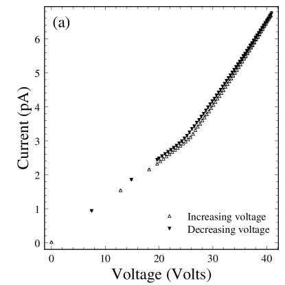
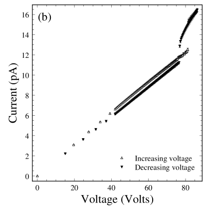
FIG. 3.: Representative current-voltage characteristics for radius ratio $\alpha=0.467$ in the absence of shear (a) and when strongly sheared (b). Note the different scales.

experimental components in a large Faraday cage which doubled as the vacuum chamber. Low noise triaxial cables and feedthroughs were used to connect the outer electrode to the electrometer.

An example of a current-voltage characteristic in a film without shear is shown in Fig. 3a. It consists of data obtained for incremental and decremental voltages. The current-voltage characteristic clearly shows two regions: one for voltages smaller than a critical voltage $V_{c}$ and one for voltages greater than $V_{c}$. The critical voltage that separates these two regions is in the vicinity of the kink in the current-voltage characteristic. In the regime $V\leq V_{c}$, the current is linearly dependent on the voltage and the film is ohmic. Experiments in 8CB with significantly higher and lower concentrations of TCNQ show, at least initially, non-ohmic current-voltage characteristics even for $V\leq V_{c}$, due to electrochemical effects.

We estimated $V_{c}$ before each run then defined an approximate reduced control parameter $\epsilon=(V/{V_{c}}^{est})^{2}-1$. Current-voltage data was then obtained by making variable steps in voltage in such a way as to make equal increments in $\epsilon$. We used several $\epsilon$ step sizes, which became finer near threshold. Similarly, we used a variable waiting time after each step, which allowed for longer relaxation times closer to $V_{c}$. Very long relaxation times were not feasible due to the drift of the electrical conductivity.[37] After the wait time, between $100-200$ measurements of the current, each separated by $25$ milliseconds, were averaged. The error in the average was taken to be the standard deviation of the mean or $1\%$, the reading error of the picoammeter, whichever was greater. Each run consisited of incrementing $\epsilon$ up to a predetermined maximum and then decrementing it to zero voltage again. Once the data had been acquired, more precise $\epsilon$ values at each voltage were found using drift-corrected values of $V_{c}$ from a fit procedure described in the next section.

When the film was sheared by rotation of the inner electrode, it was allowed at least $30$ seconds after a change of shear rate to attain a steady state before the current-voltage characteristics were obtained. In all runs, the shear rate was established and then held fixed during a current-voltage sweep. Fig. 3b displays a representative current-voltage characteristic in a film under shear. The principle effects of the shear are to suppress the onset of convection and, eventually, to make the primary bifurcation hysteretic.

IV Experimental Results

With the exception of some simple flow visualization which used slightly nonuniform films, all our results were obtained by fitting current-voltage data taken with uniform films. It is possible to fit the data in such way as to extract all the unknown material parameters in a nearly model-independent way, as well as to correct for small drifts in conductivity.

The first task was to determine the dimensionless parameters relevant to each current-voltage sweep: the radius ratio $\alpha$, the dimensionless ratio ${\cal P}$ and the Reynolds number ${\cal R}e$. We can then properly non-dimensionalize the current-voltage data and fit it to an amplitude equation model. The details of this fit are described in the section IV A below.

In Section IV B, we consider the features of the data that are predicted by the linear stability theory developed in Ref. [3]. For zero shear, these are the critical mode number $m_{c}^{0}$, and the critical voltage $V_{c}^{0}$. We use the latter to fix the last unknown material parameter, the viscosity $\eta$. We also compare our data to the linear stability prediction for the shear-suppression of the onset of convection. This was done for six values of $\alpha$, and for wide ranges of ${\cal P}$ and ${\cal R}e$.

In the weakly nonlinear regime, the value of the coefficient of the cubic nonlinearity, $g$ in the amplitude equation, was of primary interest. In Section IV C we report results for $g$ at various $\alpha$ and ${\cal P}$ for ${\cal R}e=0$, that is, in the absence of shear. We find that $g$ can become slightly negative for small $\alpha$, so that the bifurcation is weakly backward. The result for $g$ in the limit ${\cal R}e=0$, $\alpha\rightarrow 1$ is compared to the theoretical result for rectangular films[25]. Finally, in Section IV D we describe the results for $g$ in sheared films, where ${\cal R}e>0$. We find that increasing ${\cal R}e$ has a strong effect on the nature of the bifurcation, driving $g$ negative and making the bifurcation backward.

A Fitting the current-voltage data

Except for a small drift, the film is ohmic below the onset of convection. We used fits in this range to determine some important material parameters in order to scale the data.

Each voltage-current measurement in the ohmic regime, $(V,I)$, constitutes an experimental determination of the film’s conductance, $c=I/V$. For a film of radius ratio $\alpha$, thickness $s$ and conductivity $\sigma$, the conductance is given by

$$c=\frac{2\pi\sigma s}{\ln(1/\alpha)}\,.$$ (11)

Interestingly, the conductance is independent of the size of the film, i.e. independent of $r_{i}$ or $r_{o}$. Since $\alpha$ is merely a geometrical parameter, measurements of $c$ are effectively measurements of $\sigma s$, eliminating the need to determine these separately.

Using Eqn. 11, ${\cal P}$, defined in Eqn. 1, can be expressed in terms of $c$ as

$${\cal P}=\frac{\epsilon_{0}\eta}{\rho\sigma sd}=\frac{2\pi\epsilon_{0}\eta}{\rho(r_{o}-r_{i})\ln{(1/\alpha)}}~{}~{}\frac{1}{c}\,,$$ (12)

where $d=r_{o}-r_{i}$. Similarly, the Reynolds number ${\cal R}e=\rho\omega r_{i}d/\eta$ can be calculated from the measured angular frequency $\omega$ of the inner electrode in rad/s, given $\rho$ and $\eta$. The density $\rho$ of 8CB at room temperature[38] is $1.0\times 10^{3}$ kg/m³. In both ${\cal P}$ and ${\cal R}e$ , the only remaining undetermined material parameter is the viscosity $\eta$. We fixed this parameter using a combination of experimental and theoretical results, as described in Section IV B. The result was $\eta=0.18\pm 0.03$ kg/ms.

Thus, for each current-voltage sweep, we were able to determine ${\cal P}$ and ${\cal R}e$. The drift in conductivity[37] caused a drift in $c$ and hence in ${\cal P}$ over the course of a sweep. Furthermore, $c$ is only known directly during the ohmic parts at the beginning and end of each sweep. We associated a mean ${\cal P}$ with each sweep by averaging over $c$ data before and after. This results in $\sim 10\%$ errors in ${\cal P}$ for any one sweep, and a slow, uncontrolled evolution of ${\cal P}$ from sweep to sweep.

The whole range of current-voltage data is fit to the amplitude equation model. Eqn. 8 gives the full, time-dependent complex coefficient amplitude equation required by symmetry. Only the real and steady state part of Eqn. 8, given by

$$\epsilon A-gA^{3}-hA^{5}+f=0\,,$$ (13)

is required to model the current-voltage data. Here we have truncated at the quintic order and augmented Eqn. 8 with a phenomenological field term $f$. This term models the rounding of the bifurcation due to nonideal systematic effects which are slightly symmetry-breaking, resulting in an “imperfect” bifurcation.[1] For all of the fits, we found $f\ll 1$.

As discussed in section II B, the amplitude $A$ which appears in Eqn. 13 is related to the reduced Nusselt number $n$ by

$$n=\frac{I}{I_{cond}}-1=\frac{I}{cV}-1=A^{2}\,,$$ (14)

while the reduced control parameter $\epsilon$ is given by

$$\epsilon=\frac{{\cal R}}{{\cal R}_{c}}-1=\Biggl{(}\frac{V}{V_{c}}\Biggr{)}^{2}-1\,.$$ (15)

Eqns 13-15 contain five parameters, $c$, $V_{c}$, $g$, $h$, and $f$. While $c$ has a nearly constant initial slope and $V_{c}$ is marked by a relatively obvious kink in the raw $(I,V)$ data, the amplitude $A$ is indirectly deduced via the pair of transformations Eqns. 15 and 14 which are nonlinear. This amplitude is in turn fit using Eqn. 13, which is again nonlinear. Thus, the parameters $(g,h,f)$ are rather distantly related to the raw $(I,V)$ data. If $g<0$, the bifurcation is hysteretic, and $A$ is multivalued over some ranges of $\epsilon$. Also, the nature of the model necessarily involves several fit parameters which are not independent. Consequently, the determination of these parameters is much more difficult than $V_{c}$. As discussed in Sections IV C and IV D, $(g,h,f)$ can be influenced by small systematic effects in the data leading to scatter which is larger than the statistical uncertainties in the fits. Nevertheless, the general trends are robust.

The drift of the film’s conductivity, and hence its conductance $c$, introduces some additional complications. Recall that the onset of convection occurs when the control parameter ${\cal R}$ equals a critical value ${\cal R}_{c}$ given by

$${\cal R}_{c}=\frac{\epsilon_{0}^{2}{V_{c}}^{2}}{\sigma\eta s^{2}}~{}{\rm or}~{}V_{c}=\frac{s}{\epsilon_{0}}\sqrt{{\cal R}_{c}\sigma\eta}\,.$$ (16)

Since the electrical conductivity is not constant, the value of $V_{c}$ required to calculate $\epsilon$ slowly changes during the course of an experiment. Combining Eqns. 11 and 16 yields

$$V_{c}(c)=\sqrt{\frac{s\eta{\cal R}_{c}~{}{\ln(1/\alpha)}~{}c}{2\pi{\epsilon_{0}}^{2}}}\,.$$ (17)

FIG. 4.: The amplitude $A$ and the reduced Nusselt number $n=A^{2}$ vs. the control parameter $\epsilon$ for a film with radius ratio $\alpha=0.64$. The solid and dashed lines are a fit to the Landau amplitude equation.

We corrected for the drift in $c$ by tracking its value during the ohmic parts of the sweep and using a linear interpolation during the portion of the sweep where the film is convecting. In this way, each voltage and current measurement was non-dimensionalized with its own value of $c$ and $V_{c}(c)$ to produce fittable values of $\epsilon$ and $A$. We also transformed the errors in the current measurements $\Delta I$ into amplitude errors $\Delta A$.

We approached the fitting problem in the following bootstrap fashion. It was easy to ascertain bounds on $V_{c}$ by inspecting the current-voltage characteristics, see for example Figs. 3a and b. Each current-voltage characteristic was scrutinized and two voltage intervals were chosen. The first interval contained the critical voltage at which the conducting state became unstable to the convecting state. The second interval contained the voltage at which the convecting state became marginally unstable to the conduction state. Guesses of $V_{c}$ in both these intervals were chosen at random using a uniform deviate random number generator[39]. The conductances $c$ were then determined for the ohmic regimes and from a linear interpolation for the convecting portion, as described earlier. The raw current-voltage data was then transformed into $\epsilon$ and $A\pm\Delta A$ and fit to Eqn. 13 by varying only the three parameters $g$, $h$ and $f$ in a weighted Levenberg-Marquardt nonlinear fitting procedure which minimized $\chi^{2}$. We then did a Monte-Carlo optimization of the randomly chosen $V_{c}$.[39, 40]. The best $V_{c}$ was taken to be the one that minimized $\chi^{2}$ over the Monte Carlo sample. The uncertainty in $V_{c}$ was the standard deviation of the uniform deviate on the constraint interval. Corresponding to this best $V_{c}$ were the three best fit parameters

FIG. 5.: The amplitude $A$ and the reduced Nusselt number $n=A^{2}$ vs. the control parameter $\epsilon$ for radius ratio $\alpha=0.80$ with an applied shear. The solid and dashed lines are a fit to the Landau amplitude equation.

$g$, $h$ and $f$. The uncertainties in $g$, $h$ and $f$ were estimated by a Monte Carlo data decimation step with $V_{c}$ constrained to its best fit value.

For several reasons, it was necessary to restrict the fit to the neighborhood of $\epsilon\sim 0$. In the first place, amplitude equation models are only rigorously valid in the limit $\epsilon\ll 1$, although in practice they have been found to apply over a more extended range.[23] Secondly, restricting the range of $\epsilon$ reduced the impact of the residual, uncorrected component of the conductivity drift. In many cases, the drift effects were sufficiently large that only the data acquired with increasing $\epsilon$ were fit.

Figure 4 shows a typical result of transforming current-voltage data to reduced Nusselt numbers $n$ and amplitudes $A$ and fitting to Eqn. 13. The transition from conduction to convection is continuous and the best fit parameter $g>0$, indicating that the bifurcation is supercritical. Figure 5 shows the analogous result for a film under a strong shear. For this case, the transition from conduction to convection is discontinuous and $g<0$; the bifurcation is subcritical. In all fits, we found $h>0$, and $0<f\ll 1$. We performed a large number of such fits and surveyed the dependence of $g$ on $\alpha$, ${\cal P}$, and ${\cal R}e$. In addition, the fits provided determinations of the critical voltage $V_{c}$ as a function of $\alpha$, ${\cal P}$, and ${\cal R}e$ via the bootstrap process described above. These results are discussed in Sections IV C and IV D below.

B Tests of linear stability theory

This section compares the experimental measurements with the predictions of the linear stability theory given in Ref. [3].

The simplest feature of linear theory that can be compared with experiment concerns the critical mode number for zero shear, $m_{c}^{0}$. As mentioned in Section III, some experiments were performed in films with slight thickness nonuniformity. This permitted the qualitative visualization of the flow field and a quantitative determination of the mode number $m$ of the stationary pattern of vortices. Unless the bifurcation is strongly subcritical, we expect $m=m_{c}^{0}$ close to onset. The observed zero shear mode number was in excellent agreement with predictions of linear stability analysis. Table I summarizes the results. Rapid rotation of the vortex pattern and larger hysteresis prevented a systematic study of $m$ under shear. Qualitative observations confirm the general prediction that $m_{c}({\cal R}e>0)<m_{c}^{0}$, i.e. that shear reduces the number of vortices.

The primary theoretical result of Ref. [3] is the prediction of the critical voltage $V_{c}$ required for the onset of electroconvection. $V_{c}$ is given for the general case by Eqn. 16. Even though the viscosity $\eta$ is not well-known, we can test the zero shear theory for various thicknesses $s$ and conductivities $\sigma$ using the following scheme. Denoting the zero shear value of $V_{c}$ by $V_{c}^{0}$, we write

$$({V_{c}^{0}})^{2}(\alpha)=\Biggl{[}\frac{\sigma\eta s^{2}}{{\epsilon_{0}}^{2}}\Biggr{]}{\cal R}_{c}^{0}(\alpha)\,.$$ (18)

Using Eqn. 11, Eqn. 18 can be expressed more conveniently as

$$v^{2}=\frac{{4\pi^{2}\epsilon_{0}}^{2}\sigma({V_{c}^{0}})^{2}(\alpha)}{{(\ln(1/\alpha))}^{2}{\cal R}_{c}^{0}(\alpha)}=\eta c^{2}\,.$$ (19)

Written in this way, Eqn. 19 expresses a proportionality between $v^{2}$ and $c^{2}$ in which the viscosity $\eta$ is the only unknown parameter. Consistency with this proportionality over a wide range of parameters serves as a test of the linear theory for $V_{c}^{0}$ as well as a determination of $\eta$. There is one caveat: this analysis is not entirely experimental but requires the theoretical value of ${\cal R}_{c}^{0}(\alpha)$. The quantity $v$, which we refer to as the scaled critical voltage, was found as follows. For each set of current voltage data, the fit procedure outlined in Section IV A was used to deduce a critical voltage $V_{c}^{0}$ and conductance $c$ at onset. The film thickness $s$ was deduced from the color of the film. Using the measured radius ratio $\alpha$ and Eqn. 11, $\sigma$ was calculated. Finally, the numerical result for ${\cal R}_{c}^{0}(\alpha)$ was used to find $v^{2}$ which was plotted against $c^{2}$. Figure 6 shows the results obtained from $228$ current-voltage runs at six different $\alpha$, numerous different $s$ and conductivities in the range $5.9\times 10^{-8}<\sigma<8.4\times 10^{-7}{\Omega}^{-1}\rm{m}^{-1}$. Consequently, the range of ${\cal P}$ is very broad.

FIG. 6.: The scaled critical voltage vs. the square of the conductance for various films at six different $\alpha$. The solid line is a one-parameter fit with a single constant of proportionality which determines the viscosity $\eta=0.18\pm 0.03$ kg/ms.

Within some scatter, Fig. 6 exhibits the predicted proportionality over several decades. Hence, the theory properly accounts for the scaling of the critical voltage with respect to the film thickness and radius ratio.

A single-parameter linear fit to $v^{2}=\eta c^{2}$ gives $\eta=0.18\pm 0.03$ kg/ms. This is a reasonable value for the viscosity; while it has not been independently measured, it is believed to be of order of $0.1$ kg/ms.[41]

We now turn to the case of nonzero shear. The main prediction of the linear stability analysis is that the onset of electroconvection is suppressed by Couette shear. This suppression is both $\alpha$ and ${\cal P}$ dependent. Returning to Eqn. 2, the degree of suppression $\tilde{\epsilon}$ is given by

$$\tilde{\epsilon}~{}(\alpha,{{\cal R}e},{\cal P})=\Biggl{[}\frac{{\cal R}_{c}(\alpha,{{\cal R}e},{\cal P})}{{\cal R}_{c}^{0}(\alpha)}\Biggr{]}-1=\Biggl{(}\frac{V_{c}(\alpha,{\cal R}e)}{V_{c}^{0}(\alpha)}\Biggr{)}^{2}-1\,.$$ (20)

We used the two equivalent expressions for $\tilde{\epsilon}$ in Eqn. 20 to calculate the suppression theoretically and experimentally. $V_{c}(\alpha,{\cal R}e)$ was found from the nonlinear fit, along with the conductance $c$ for that particular sweep. It was necessary to correct $V_{c}^{0}(\alpha)$ for the drift of $c$ in order to calculate $\tilde{\epsilon}$. This was done using values of $V_{c}^{0}(\alpha)$ taken from zero shear sweeps performed before and after each sheared sweep. The variation of $V_{c}^{0}(\alpha)$ with $c$ was modelled with a linear fit which was used to find the drift-corrected value of $V_{c}^{0}(\alpha)$. In this way each experimental value of $\tilde{\epsilon}$ could be be computed for a constant $c$. The uncertainty in $\tilde{\epsilon}$ was dominated by the uncertainty

FIG. 7.: A comparison between the measured suppression $\tilde{\epsilon}$ vs. ${\cal R}e$ and the predictions of local and nonlocal theory based on Ref. [3]. In (a) $\alpha=0.47$. The different symbols denote the ${\cal P}$-quartiles: $13.3<\circ<15.4<\bullet<17.5<\Box<19.6<\triangle<21.7$. The theoretical lines are for the mean ${\cal P}=16.3$ of the data. Similarly, in (b) $\alpha=0.64$, $29.1<\circ<37.1<\bullet<45.2<\Box<53.2<\triangle<61.2$ and the theoretical lines are for the mean ${\cal P}=45.2$. Note the very different scales.

in the drift correction to $V_{c}^{0}$. The conductance $c$ for each $\tilde{\epsilon}$ can be used to calculate its associated value of ${\cal P}$. Thus, we arrive at sets of experimental values of $\tilde{\epsilon}(\alpha,{{\cal R}e},{\cal P})$ for fixed $\alpha$ and ${{\cal R}e}$ and ranges of ${\cal P}$. These can be compared in detail to the theoretical results for suppression as a function of these parameters given in Ref. [3, 42]. Figures 7a and b show this comparison at $\alpha=0.47$ and $\alpha=0.64$ respectively. In each case the theoretical curves are calculated for the mean value of the range of ${\cal P}$ spanned by the data. For a discussion of the distinction between the local and nonlocal approximations, see Ref. [3].

Note that the ranges of ${\cal R}e$ for these two $\alpha$ are different by a factor of ten and that the suppressions are also very different. It is quite interesting that a rather mild shear (${{\cal R}e}\sim 3)$ suppresses the onset of electroconvection so strongly that $\tilde{\epsilon}\sim 14$ (i.e. ${\cal R}_{c}=15{\cal R}_{c}^{0}$). We have also studied the suppression at $\alpha=0.33,0.56,0.60$, and $0.80$. The results are similar to Fig. 7. The suppression data covers the range $10<{\cal P}<130$ and $0\leq{\cal R}e<3$. In each case the agreement between theory and experiment is fair, with the theory slightly underestimating the suppression in most cases. The upper bound on ${\cal R}e$ could easily be extended using increased rotation rates, while smaller ${\cal P}$ would require larger, thicker films.

The degree of agreement shown in Figs. 7 is essentially independent of the value of $\eta$. Recall that $\eta$ was determined by a single parameter fit to Eqn. 19. Since the $\eta$ dependence in the ${\cal R}e$ scaling of both the theory and the experiment are proportional to $1/\eta$, any change in $\eta$ multiplies both by the same factor.[3] This simply results in a rescaling of the ${\cal R}e$ axis in Figs. 7a and b, with no change in the quality of the agreement.

We close this section with some brief speculation on what might account for the scatter in Fig. 6 and for the remaining discrepancies between theory and experiment in the suppression curves.

The most likely sources of these discrepancies are the imperfect geometry of the film and its finite thickness. The 2D theoretical model assumed that the flow velocity is independent of position over the thickness of the film. This may be inexact for thicker films. Since the electrical forcing is localized near the free surfaces, it seems likely that the surfaces are preferentially driven in thick films so that the motion is not accurately 2D. The film’s edges are also imperfect because small wetting layers unavoidably exist on the circumferences of the inner and outer electrodes. These may produce electrical or velocity boundary conditions that are not exactly those assumed by the theory. In general, however, the linear stability theory works remarkably well considering its rather simple assumptions.

C Coefficients of the Cubic Nonlinearity without Shear

In this section, we consider the experimental results in the nonlinear regime, beginning with the unsheared ${\cal R}e=0$ case. These are expressed in terms of the cubic Landau coefficient $g$ of the amplitude equation, Eqn. 13. Even with ${\cal R}e$ fixed at zero, we will show that this coefficient is an interesting and nontrivial function of the remaining dimensionless quantities, ${\cal P}$ and $\alpha$.

The radius ratio $\alpha$ is a fixed geometric parameter for each run, determined only by the choice

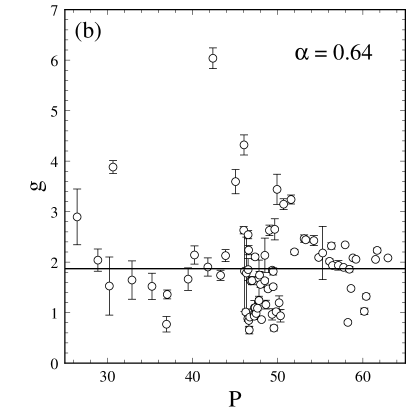
FIG. 8.: (a) Measurements of the coefficient of the cubic nonlinearity $g$ for zero shear vs. ${\cal P}$ for (a) $\alpha=0.33$ and (b) $\alpha=0.64$.

of the electrode dimensions. The ${\cal P}$ appropriate to each film was deduced after each run as described in Section IV A. Since ${\cal P}$ is proportional to the conductivity, which exhibits a slow drift, a wide range of ${\cal P}$ could be investigated. While they are independent in principle, $\alpha$ and ${\cal P}$ are not easy to separate experimentally. This practical constraint derives from Eqn. 12 in which ${\cal P}\propto d^{-1}$, where the width of the film $d=r_{o}-r_{i}$. In practice, $d$ is largest at small $\alpha$, so the runs with the smallest ${\cal P}$ occur for small $\alpha$.

The nonlinear coefficient $g(\alpha,{\cal P})$ was determined as described in Section IV A. Figures 8a and b show $g$ as a function of ${\cal P}$ for two different $\alpha$. The scatter that is manifest in these plots exceeds the statistical uncertainty of the fit. As discussed in Section IV A, the scatter originates from systematic effects due to the non-ideal features of the experiment. Nevertheless, the gross features of the ${\cal P}$ dependence of $g$ can still be extracted.

At $\alpha=0.33$, the measurements explored the range $2<{\cal P}<8$. These were the smallest ${\cal P}$ reached in the experiment. It is clear from Fig. 8a that $g$ increases with ${\cal P}$, and passes through zero for small enough ${\cal P}$. Thus, for $\alpha=0.33$, we find that the bifurcation from the conduction state to the $m=4$ vortex state is subcritical ($g<0$) for ${\cal P}\stackrel{{\scriptstyle<}}{{\sim}}5$ and supercritical ($g>0$) for ${\cal P}\stackrel{{\scriptstyle>}}{{\sim}}5$. Near ${\cal P}\stackrel{{\scriptstyle\sim}}{{=}}5$ we pass a tricritical point. It is interesting to observe that in each case the bifurcation involves the same two symmetry states, yet its subcriticality depends on ${\cal P}$.

For all the other, larger $\alpha$ investigated, $g$ was found to be independent of ${\cal P}$. This is illustrated in Fig. 8b for $\alpha=0.64$ and was also true for $\alpha=0.47,~{}0.56,~{}0.60,$ and $0.80$. However, for all of these cases, ${\cal P}$ was never less than $10$ and can be as large as several hundred. Thus, it is unclear whether the subcriticality at $\alpha=0.33$ is due to the smallness of ${\cal P}$ or the smallness of $\alpha$, or some combination. It would be interesting to determine whether $g$ also becomes negative for large $\alpha$ as ${\cal P}$ decreases. The regime of large $\alpha$ and small ${\cal P}$, while accessible in principle, would require significantly larger electrodes or much thicker films. All electroconvection experiments on freely suspended films in the rectangular geometry have reported supercritical bifurcations[20, 21, 22, 23]. However, these experiments were also at large ${\cal P}$ and so the possibility of a subcritical bifurcation in rectangular films cannot be excluded.

The case of large ${\cal P}$ is easier to understand. In the governing electrohydrodynamic equations (see Ref. [3]), the parameter analogous to the Prandtl number only appears as the inverse, ${\cal P}^{-1}$, multiplying certain nonlinear terms. Hence, it is perhaps not surprizing that $g$ becomes independent of ${\cal P}$ for ${\cal P}\stackrel{{\scriptstyle>}}{{\sim}}10$, where these terms become negligible.

In order to examine how $g$ depends on $\alpha$, we removed the ${\cal P}$ dependence by averaging over data at various ${\cal P}$. For the five largest $\alpha$, $g$ is independent of ${\cal P}$ over broad ranges of ${\cal P}$. A weighted average of $g$ was obtained for these cases. For $\alpha=0.33$, where some ${\cal P}$ dependence was evident, only $g$ values in the narrow range $2.1<{\cal P}<4.4$ were averaged.

In this averaging the systematic scatter in $g$ was treated as random. It is thus likely that the true uncertainty in the average values of $g$ will be much larger than the standard deviation of the mean. The ultimate test of this procedure lies in the comparison of the averaged values of $g$ with theoretical predictions. As we describe below, the limited comparison we are able to make at present is not unfavourable. The line in Fig. 8b shows the average value of $g$ for the plotted data. All of the results for $g(\alpha)$ are tabulated in Table II and plotted in Fig. 9.

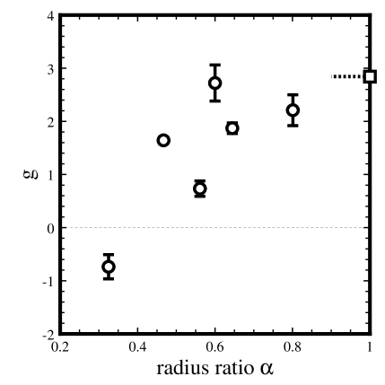
FIG. 9.: Measurements of the coefficient of the cubic nonlinearity $g$ for zero shear vs. the radius ratio $\alpha$. The dashed line shows the theoretical value for $g$ in the limits ${\cal P}\rightarrow\infty$ and $\alpha\rightarrow 1$ from Ref. [25].

It is clear from Fig. 9 that, overall, $g(\alpha)$ increases with $\alpha$. As discussed above, the larger $\alpha$ data are also associated with larger ${\cal P}$. At present, no theoretical predicion is available for $g$ at arbitrary $\alpha$ and ${\cal P}$. However, we expect $g$ to approach a limiting value quite rapidly as $\alpha\rightarrow 1$. This limit corresponds to an unbounded lateral geometry in which the film is a strip of fluid suspended at its long parallel edges by two semi-infinite plate electrodes. In this limit the discrete azimuthal mode numbers $m$ are replaced by a continuous wavenumber $k=m/{\bar{r}}$, where ${\bar{r}}=(r_{i}+r_{o})/2$ is the mean radius. From linear theory, we found that the critical parameters ${\cal R}_{c}^{0}$ and $k_{c}^{0}=m_{c}^{0}/{\bar{r}}$ at $\alpha=0.80$ are already very close to the limiting values for $\alpha\rightarrow 1$.[3]

This limiting behaviour is reasonable given the large dimensionless circumference for large $\alpha$. The relevant aspect ratio $\Lambda$ is the circumference at the mean film radius, $\pi(r_{i}+r_{o})$, divided by the width of the film $d=r_{o}-r_{i}$, so that $\Lambda=\pi(1+\alpha)/(1-\alpha)$. At $\alpha=0.80$, $\Lambda\sim 28$. Almost all the experiments performed in the rectangular geometry had $\Lambda\stackrel{{\scriptstyle<}}{{\sim}}10$ [20, 21, 22, 23, 24] and were well-modelled by the theory for an unbounded strip for which $\Lambda=\infty$. It is thus resonable to expect $g$ at $\alpha=0.80$ to be close to its limiting value for $\alpha=1$. Similarly, as the large $\alpha$ data also involve very large values of ${\cal P}$, we may also employ the theory in the ${\cal P}\rightarrow\infty$ limit.

Weakly nonlinear analysis of unsheared electroconvection in the ‘plate’ electrode geometry was presented in Ref. [25] for the case ${\cal P}=\infty$. The result of that analysis, $g=2.842$ is shown in Fig. 8. It is in good agreement with a reasonable extrapolation of the data to the $\alpha\rightarrow 1$ limit.

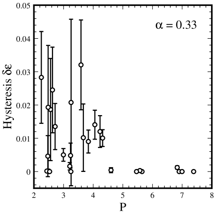
FIG. 10.: Measurements of the hysteresis width $\delta\epsilon$ vs. ${\cal P}$

for radius ratio $\alpha=0.33$.

When $g<0$, the onset of convection becomes hysteretic and the quintic term with coefficient $h$ in Eqn. 13 becomes significant.[42] Since $0<f\ll 1$, the width of the hysteresis loop $\delta\epsilon$ in $\epsilon$ is given by $\delta\epsilon=g^{2}/4h$. When $g\geq 0$, $\delta\epsilon=0$. The hysteresis width with zero applied shear is plotted in Fig. 10 for $\alpha=0.33$ and various ${\cal P}$. Note that the hysteresis vanishes for ${\cal P}\stackrel{{\scriptstyle>}}{{\sim}}5$ and even when non-zero, is always rather small, $\delta\epsilon\sim 0.02$. This is in contrast with the sheared case, discussed in the next Section, for which $\delta\epsilon\sim 0.1$.

D Coefficients of the cubic nonlinearity with shear

In the presence of shear, the coefficient $g$ of the cubic nonlinearity is strongly dependent on the Reynolds number ${\cal R}e$ of the Couette flow imposed in the base state. We find that the shear drives $g$ negative, producing a hysteretic Hopf bifurcation to convection in the form of travelling vortices. In this Section, we describe the ${\cal R}e$ dependence of $g$, which, as in the previous Section, is also a function of the radius ratio $\alpha$ and the dimensionless ratio ${\cal P}$.

Figure 11 shows a representative example of the ${\cal R}e$ dependence of $g$, in this case for $\alpha=0.47$. At ${\cal R}e=0$, the value of $g$ is found, as described in Section IV C, by averaging over a range of ${\cal P}$, which was always $>10$. In the case shown in Fig. 11, $g({\cal R}e=0)=1.64\pm 0.06$ with a mean ${\cal P}$ of $16.3$. The plotted $g$ data for ${\cal R}e>0$ had $13.3<{\cal P}<21.7$.

Our main result is that ${\cal R}e$ plays the part of a second control parameter which allows the primary bifurcation

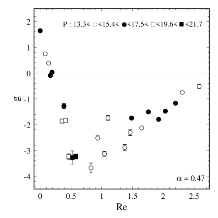
FIG. 11.: Measurements of the coefficient of the cubic nonlinearity $g$ vs. the Reynolds number ${\cal{R}}e$ at $\alpha=0.47$. The different symbols denote data in various quartiles of ${\cal P}$.

to electroconvection to be tuned between super- and subcritical. For $\alpha=0.47$, the bifurcation is supercritical at ${\cal R}e=0$ and weakens as the Reynolds number increases. The bifurcation becomes tricritical at ${\cal R}e\sim 0.2$ and is subcritical thereafter. The subcriticality at first deepens with increasing Reynolds number, until at ${\cal R}e\sim 0.85$ a minimum value of $g\stackrel{{\scriptstyle\sim}}{{=}}-3.7$ is reached. For ${\cal R}e>0.85$, the bifurcation remains subcritical but $g$ becomes an increasing function of the Reynolds number. For the range of Reynolds numbers investigated the bifurcation does not become supercritical again.

There is some scatter in the data, nonetheless, the overall trends are clear. The systematic deviations are comparable to those in Figs. 8a and b. The results were qualitatively similar for $\alpha=0.56,0.60,0.64,$ and $0.80$. The tricritical Reynolds number at which $g=0$ will be denoted ${{\cal R}e_{T}}$. The value of ${{\cal R}e_{T}}$ varys for different $\alpha$ and ${\cal P}$, but the general features of the $g$ vs. ${\cal R}e$ curve are preserved over a wide range of parameters. Table III lists the values of ${\cal R}e_{T}$ under various conditions.

The variation of ${\cal R}e_{T}$ is probably due to the combination of changing both $\alpha$ and ${\cal P}$, rather than to the variation either parameter separately. These are difficult to experimentally disentangle and the parameter space is large. For zero shear, $g$ was found to be independent of ${\cal P}$ for ${\cal P}\stackrel{{\scriptstyle>}}{{\sim}}10$, but under shear there is insufficient data to draw many conclusions about the ${\cal P}$ dependence of $g$. If linear theory is any guide, we expect there will in general be a greater ${\cal P}$ dependence in the sheared case. It was established in Ref. [3] that the linear theory result for ${\cal R}_{c}$ was independent of ${\cal P}$ for ${\cal R}e=0$,

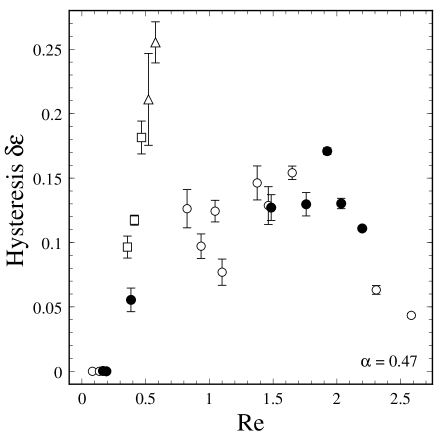
FIG. 12.: The hysteresis width $\delta\epsilon$ vs. the Reynolds number ${\cal R}e$ for radius ratio $\alpha=0.47$. The symbols denote the same quartiles of ${\cal P}$ as in Fig. 11.

but weakly dependent on ${\cal P}$ for ${\cal R}e\neq 0$. It appears from the tabulated results that as ${\cal P}$ and $\alpha$ decrease, ${\cal R}e_{T}$ increases.

The minimum value of $g$ as a function of ${\cal R}e$ also vary for different $\alpha$ and ${\cal P}$. We will refer to the coordinates of this special point as $g_{min}$ and ${\cal R}e_{min}$. Table IV lists the minimum values observed. A look at Fig. 11 shows that the minimum value is only known up to the density of data and to within the scatter in the whole plot. The minimum is a local one and is observed within ranges of ${\cal R}e$ which had different maxima for different $\alpha$.

Since the parameter space for the data is defined by several parameters it becomes difficult to make meaningful comparisons of the experimental results when more than one parameter changes. However, one fortunate comparison can be gleaned from Table IV. At $\alpha=0.47$, the film had ${\cal P}=15.3$ while at $\alpha=0.80$, ${\cal P}=12.0$. Since the radius ratios are very different and the ${\cal P}$ are not, it is not unreasonable to directly compare the values of $g_{min}$ and ${\cal R}e_{min}$ for these cases. It is evident that the bifurcation is much more strongly subcritical at $\alpha=0.80$ than at $\alpha=0.47$, and the values of ${\cal R}e_{min}$ are also very different.

The coefficient of the quintic nonlinearity $h$ as function of ${\cal R}e$ is studied in Ref. [42]. Figure 12 shows the the hysteresis width $\delta\epsilon=g^{2}/4h$ as a function of ${\cal R}e$ for $\alpha=0.47$. The hysteresis when ${\cal R}e>0$ is much larger than that described in the previous Section which was found for ${\cal R}e=0$ at small $\alpha$ and ${\cal P}$.

The Nusselt number of the convection is independent of the Hopf frequency (i.e. the travelling rate of the vortex pattern). It would be interesting to measure this frequency, which is governed by the imaginary part of the complex Ginzberg-Landau equation, Eqn. 10, and depends on $\epsilon$, $\alpha$, ${\cal R}e$ and ${\cal P}$. This would however require visualization of the flow pattern or some spatially localized probe of the amplitude.

V Discussion

Because of its rather simple symmetry and forcing scheme, annular electroconvection under applied shear has many similarities to other systems and models. In this section, we discuss these similar systems with a view to putting annular electroconvection into a general context.

Electroconvection is obviously analogous to buoyancy-driven thermal convection. In fact, it can be shown that the linear stability problem for surface charge driven electroconvection in thin films reduces to the 2D Rayleigh-Bénard problem if the nonlocal coupling between fields and charges is neglected.[7] Detailed calculations show that this “local” approximation is an accurate one, even when applied in the weakly nonlinear regime.

There have been some theoretical studies of 3D Rayleigh-Bénard convection (RBC) in the presence of a plane Couette shear flow[43]. The theory assumed the usual theoretical geometry of a fluid layer confined between infinite, perfectly conducting horizontal planes. Our annular system approaches the plane one in the $\alpha\rightarrow 1$ limit. (The $\alpha<1$ annular geometry has finite extent and curvature; the implications of these are discussed below.) Linear stability analysis of a plane Couette base state to RBC reveals stability differences between transverse roll disturbances (with axes perpendicular to the shear flow), and longitudinal roll disturbances (with axes parallel to the shear flow). Longitudinal-roll disturbances have identical stability properties to unsheared RBC, and are always more unstable than the transverse-roll disturbances. In fact, longitudinal-roll disturbances have stability properties that are independent of any uni-directional shear flow along the axis of the rolls. In our 2D system, these more unstable longitudinal roll modes do not exist and the vortices we see correspond to truly 2D transverse rolls. Thus, we observe the analog of a state that would normally be preempted by longitudinal rolls if the geometry were not constrained.

According to linear theory, transverse-roll disturbances in unbounded, sheared RBC, like our vortices, exhibit suppression, or added stability due to the shear, under plane Poiseuille or plane Couette or any mixture of these two flows. The onset Rayleigh number for transverse rolls is a monotonically increasing function of the shear Reynolds number, similar to what we found for electroconvection. Furthermore, the critical wavenumber of the most unstable transverse disturbance was found to be a monotonically decreasing function of the shear Reynolds number, which is analogous to the reduction of $m_{c}$ by shear that we observed. Transverse rolls also travel under unidirectional plane Couette shear, again analogous to our travelling vortex state.

Whereas unbounded RBC with plane Couette shear cannot be realized experimentally, RBC has been studied experimentally and theoretically in narrow slots with open through-flows.[1, 44, 45] Quasi-2D transverse rolls can be stabilized by wall effects in slots. The through-flow consists of a weak Poiseuille flow with a very small Reynolds number. Its effects on RBC are well understood. In brief, the onset of convection is again suppressed, but the first instability is convective (i.e. it grows only downstream of a localized perturbation), rather than absolute. The resulting convection pattern drifts in the direction of the through flow. It is interesting that the clear distinction between convective and absolute instability is blurred in annular electroconvection with shear, in which the ‘through’ flow loops back on itself. The annular geometry is naturally closed. The linear stability analysis of Ref. [3] only treated absolute instablity. In principle, the system might still be considered to be convectively unstable if localized perturbations grew only as they travelled azimuthally.

Taylor Vortex flow (TVF)[1] is an extensively studied pattern-forming instability with geometric similarities to annular electroconvection. However, the instability leading to TVF depends crucially on axial disturbances to 3D Couette flow. Purely 2D circular Couette flow is, in fact, linearly stable.[46, 47] TVF is the result of an instability of a 3D shear flow, while what we have studied here is the effect of a shear flow on the electroconvective instability.

Agrait and Castellanos theoretically studied the effect of a 3D Couette shear on an electrohydrodynamic instability in TVF geometry.[16] Their electrohydrodynamic system consisted of a nearly insulating fluid confined between metallic electrodes. Charge injection, a process by which charge carriers are created at the electrodes, occurs when strong electric fields are applied. The interaction of this volume charge density with the applied electric field leads to electroconvection instabilities.[14, 15, 17] Agrait and Castellanos considered electroconvection due to a radial field with charge injection on either cylinder. Both cylinders were permitted to rotate to produce a general Couette shear. They found that shearing enhanced the instability, leading to a 3D flow that resembles TVF. This is in direct contrast to the stabilizing effects we observed in 2D.

Although shear and rigid rotation are conceptually quite different, it is interesting to compare their effects on instabilities. Again, we find crucial distinctions between 2D and 3D systems.

The added stability in sheared annular electroconvection is a consequence of the shear and not of rotation. Under rigid rotation, where the inner and outer electrodes are co-rotating, one can transform to rotating co-ordinates in which the electrodes are stationary. This transformation introduces a Coriolis term $-2\Omega\hat{\bf z}\times{\vec{\bf v}}=-2\Omega\nabla\psi$ in the Navier-Stokes equation which may be absorbed into the pressure gradient term $\nabla P$ and eliminated.[3, 30] Thus, in a purely 2D system, rigid rotation and the non-rotating, unsheared case have identical stability. It also follows, since the transformation is general and the unsheared bifurcation is stationary, that the resulting nonlinear vortex pattern above onset must be stationary in the co-rotating frame.

This lack of dependence on rigid rotation may be contrasted with a large class of 3D and quasi-2D rotating Rayleigh-Bénard systems[4, 48, 49, 50, 51, 52], where rotation produces added stability but the absence of strictly 2D flow results in a time-dependent (precessing) convection pattern in the co-rotating frame. The precession seen in these systems is analogous to the travelling of the sheared patterns that we observed only to the extent that rotation and shear break the same symmetry, which allows travelling patterns. Symmetry aside, the physical origins of added stability and precession are fundamentally different between the 2D sheared and 3D rotating cases.

In general, 3D rotating convecting systems may also support strictly 2D ‘Taylor column’[53] solutions which do not precess in the rotating frame and whose onset occurs at the same critical Rayleigh number as in the absence of rotation.[4, 30] The system most analogous to ours is the interesting but experimentally unrealizable situation of 2D RBC in a rotating annular geometry with purely radial gravity and heating[30]. Theoretical studies found columnar solutions which are very closely analous to our vortices. One might hope to approach this limit in experiments using radially temperature gradients imposed between rapidly rotating concentric cylinders. Purely columnar solutions have not observed in any rotating RBC experiment because the boundary conditions at the top and bottom of the cylinder must be stress free[4, 30], a requirement that cannot be attained in terrestrial RBC experiments. In contrast, two-dimensionality, stress free surface conditions and radial driving forces all arise naturally in the electroconvection of an annular suspended film. Thus, the vortices that occur in annular electroconvection without shear are accurate 2D analogs of ‘Taylor columns’.

The similarity between our system and many other better-studied systems and models suggests that many linear and nonlinear techniques developed for other problems can be fruitfully brought to bear on annular electroconvection. In addition, the system may allow the study of bifurcation scenarios that are not experimentally realizable in other similar systems.

.

VI Conclusion

In this paper, we have reported a wide ranging experimental study of the primary bifurcation to electroconvection in sheared two-dimensional annular films. Our principal experimental probe was the excess current carried by the film due to convection, which can be directly related to the amplitude of the convective flow. In all, we examined annuli with six different radius ratios $\alpha$, with $0.33~{}\leq~{}\alpha~{}\leq~{}0.80$. For these, the Reynolds number of the applied Couette shear varied between $0~{}\leq~{}{\cal R}e~{}<~{}3$. The explored range for the dimensionless parameter ${\cal P}$, which varies with film thickness and conductivity, was $1~{}<~{}{\cal P}~{}<~{}150$.

We compared this data, in the first instance, with the predictions of linear theory[3]. The data for the critical voltage $V_{c}^{0}$ for the onset of convection without shear could be combined for all six radius ratios and was shown to obey the scaling predicted by linear theory. This data could then be used in a slightly model-dependent way to fix the only remaining unknown material parameter, the fluid viscosity. We could then compare the experimentally measured suppression of the onset by shear to linear theory in an essentially pararmeter-free way. The agreement was satisfactory for a wide range of $\alpha$, ${\cal P}$, and ${\cal R}e$. Using a simple visualization scheme, we also confirmed that the azimuthal mode number $m$ near onset was close to the most unstable critical value $m_{c}$ predicted by linear theory.

Nonlinear fits to current-voltage data above the onset of convection were then used to infer the real part of the amplitude of convection. Under shear, the amplitude can be shown to obey a complex Ginzburg-Landau equation; its real part was fit to the time-independent steady state version of this equation in order to extract the coefficient $g$ of the cubic nonlinearity. When shear is absent, the primary bifurcation is a pitchfork while with shear, the bifurcation is a pitchfork Hopf. We determined the functional dependence of $g$ as $\alpha$, ${\cal R}e$ and ${\cal P}$ were varied. When shear is absent, it was found that for $\alpha=0.47,0.56,0.60,0.64,0.80$ and ${\cal P}\stackrel{{\scriptstyle>}}{{\sim}}13$ that $g$ was independent of ${\cal P}$. In addition, in this regime $g~{}>~{}0$, hence the bifurcation was supercritical. For $\alpha~{}=~{}0.33$, $g$ was found to be an increasing function of ${\cal P}$ for $2~{}<~{}{\cal P}~{}<8$. More importantly, it was found that the bifurcation was subcritical($g~{}<0$) for ${\cal P}\stackrel{{\scriptstyle<}}{{\sim}}5$ and supercritical($g~{}>0$) for ${\cal P}\stackrel{{\scriptstyle>}}{{\sim}}5$. In overall trend, we found that $g$ is an increasing function of $\alpha$ for zero shear. The largest $\alpha=0.80$ was sufficiently close to the limiting case of $\alpha\rightarrow 1$ that we could extrapolate the measured values of $g$ for comparison to the value of $g$ calculated from weakly nonlinear theory for the corresponding ‘plate’ electrode geometry. This quantitative comparison gave reasonable agreement.

When shear was applied, it had a strong effect on the subcriticality of the primary bifurcation. Measurements of $g$ as a function of the shear Reynolds number ${\cal R}e$ revealed that for $\alpha=0.47,0.56,0.60,0.64,0.80$ there existed a tricritical Reynolds number ${\cal R}e_{T}$ below which $g>0$ and the onset is a supercritical Hopf bifurcation. For ${\cal R}e>{\cal R}e_{T}$, $g<0$ and the onset became a subcritical Hopf bifurcation with the degree of subcriticality a nontrivial function of ${\cal R}e$. Hence, the Reynolds number forms an interesting second control parameter in this system which can be used to vary the nature of the primary bifurcation.

The data presented in this paper represents only a sparse sampling of the full 3D parameter space of $g(\alpha,{\cal P},{\cal R}e)$. Within this space, there presumably exist continuous 2D loci on which $g=0$ and the primary bifurcation is tricritical. On other loci, the hysteresis $\delta\epsilon$ is a local maximum. As a function of $\alpha$, linear theory[7] shows that there exist special values of $\alpha$ at which two azimuthal mode numbers $m$ and $m+1$ are simultaneously linearly unstable. All of the $g$ results we have described pertain to the primary bifurcation; above onset we also observed numerous secondary bifurcations which take the form of hysteretic jumps in $m$. The location of these secondary bifurcations is a function of ${\cal R}e$. These considerations suggest that more-or-less discontinuous jumps in the behavior of $g$ may occur at parameter values across which the azimuthal mode number $m$ of the nonlinear pattern changes discontinuously. The rich phenomenology of even the primary bifurcation presents a significant challenge to the weakly nonlinear theory of this instability.

REFERENCES

- [1] M. C. Cross and P. C. Hohenberg, Rev. Mod. Phys. 65, 851 (1993).
- [2] A.C. Newell, T. Passot and J. Lega, Ann. Rev. Fluid Mech., 25, 399 (1993).
- [3] Z.A. Daya, V. B. Deyirmenjian, and S. W. Morris, Phys. Fluids, 11, 3613 (1999).
- [4] E. Knobloch, in Lectures on Solar and Planetary Dynamos edited by M. R. E. Proctor and A. D. Gilbert (Cambridge University Press, New York, 1994), p. 331.
- [5] V. B. Deyirmenjian, Z. A. Daya, and S. W. Morris, unpublished.
- [6] Z.A. Daya, V. B. Deyirmenjian, S. W. Morris, and J. R. de Bruyn, Phys. Rev. Lett. 80, 964 (1998).
- [7] Z. A. Daya, S. W. Morris, and J. R. de Bruyn, Phys. Rev. E 55, 2682 (1997).
- [8] A. A. Sonin, Freely suspended liquid crystalline films (John Wiley, Chichester, New York, 1998).
- [9] D. Dash and X.L. Wu, Phys. Rev. Lett. 79, 1483 (1997).
- [10] Y. Couder, J.M. Chomaz and M. Rabaud, Physica D 37, 384 (1989).
- [11] D. Avsec and M. Luntz, Compt. Rend. Acad. Sci. (Paris) 203, 1140 (1936).
- [12] W. V. R. Malkus and G. Veronis, Phys. Fluids 4, 13 (1961).
- [13] D.C. Jolly and J. R. Melcher, Proc. Roy. Soc. London A., 314, 269 (1970).
- [14] J. R. Melcher, Continuum Electromechanics (MIT Press, Cambridge MA, 1981).
- [15] N. J. Felici, J. Phys. (Paris) Colloq. 37, C1-11 (1976).
- [16] N. Agrait and A. Castellanos, Physico-Chemical Hydrodynamics, 10, 181 (1988).
- [17] A. T. Pérez and A. Castellanos, Phys. Rev. A 40, 5844 (1989).
- [18] S. Faetti, L. Fronzoni, and P. Rolla, J. Chem. Phys. 79, 5054 (1983).
- [19] A. Buka and L. Kramer, Pattern Formation in Liquid Crystals, (Springer, Berlin, 1995).
- [20] S. W. Morris, J. R. de Bruyn, and A. D. May, Phys. Rev. Lett. 65, 2378 (1990).
- [21] S. W. Morris, J. R. de Bruyn, and A. D. May, J. Stat. Phys. 64, 1025 (1991).
- [22] S. W. Morris, J. R. de Bruyn, and A. D. May, Phys. Rev. A 44, 8146 (1991).
- [23] S. S. Mao, J. R. de Bruyn, and S. W. Morris, Physica A 239, 189 (1997).
- [24] S. S. Mao, J. R. de Bruyn, Z. A. Daya, and S. W. Morris, Phys. Rev. E 54, R1048 (1996).
- [25] V. B. Deyirmenjian, Z. A. Daya, and S. W. Morris, Phys. Rev. E, 56, 1706 (1997).
- [26] S. Ried, H. Pleiner, W. Zimmermann, and H. R. Brand, Phys. Rev. E, 53, 6101 (1996).
- [27] A. Becker, S. Ried, R. Stannarius, and H. Stegemeyer, Europhys. Lett. 39, 257 (1997).
- [28] C. Langer and R. Stannarius, Phys. Rev. E., 58, 650 (1998).
- [29] C. Langer, Z. A. Daya, S. W. Morris and R. Stannarius, to be published in Mol. Cryst. Liq. Cryst.
- [30] A. Alonso, M. Net, and E. Knobloch, Phys. Fluids, 7, 935 (1995).
- [31] It was also found that the critical azimuthal mode number under shear is reduced so that .
- [32] Samples with high concentrations of TCNQ, left to themselves for a period of weeks to months, changed color from off-white to orange to green. The same changes were observed in a solution of TCNQ in acetonitrile independent of concentration. At the lower dopant concentrations used in the experiments, the samples remained an off-white color.
- [33] G. Wyszecki, Colorimetry, in Handbook of Optics, McGraw-Hill (1978).
- [34] A. Nemcsics, Colour Dynamics (Ellis Horwood, New York, 1993).
- [35] E. B. Sirota, P. S. Pershan, L. B. Sorensen and J. Collett, Phys. Rev. A, 36, 2890 (1987).
- [36] A.J. Leadbetter, J.C. Frost, J.P. Gaughan, G.W. Gray, and A. Mosly, J. Phys. (Paris) 40, 375 (1979).
- [37] It is well known that liquid crystals degrade upon dc excitation; see for example S. Barret, F. Gaspard, R. Herino, and F. Mondon, J. Appl. Phys. 47, 2375 (1976). The changes in the electrical conductivity of our liquid crystal film are due to electrochemical reactions with the electrodes. The presence of suitable dopants is known to arrest the degradation process, nonetheless the electrochemical reactions with the electrodes slowly change the film conductivity. It is for this reasson that the ohmic portions of the current-voltage characteristics of the incremental and decremental runs in Figs. 3a and b do not coincide. The drift in the conductivity was usually but ranged up to during the course of an experimental run of minutes duration. The drift had no simple time dependence under any of the experimental conditions and was clearly a complex process. Relaxation times for obtaining the current-voltage characteristics were never in excess of seconds so as to contain the total drift during an experimental run. While the drift in the conductivity is inconvenient, it can be corrected for in the data as described in Section IV A. Surprisingly however, the drift in the conductivity facilitates the exploration of a much broader range of the parameter space of the experiment. One of the parameters introduced earlier was . The drift in the conductivity makes accessible a wide range of without having to draw a film of different thickness or with a different dopant concentration.
- [38] D. A. Dunmur, M. R. Manterfield, W. H. Miller and J. K. Dunleavy, Mol. Cryst. Liq. Cryst. 46, 127 (1978).
- [39] W. H. Press, S. A. Teukolsky, W. T. Vetterling, and B. P. Flannery, Numerical Recipes in C, (Cambridge University Press, Cambridge, 1992).
- [40] L.E. Scales, Introduction to Nonlinear Optimization (Macmillan Publishing Ltd., London, 1985).
- [41] R.G. Horn and M. Kleman, Ann. Phys., 3, 229 (1978).
- [42] Z. A. Daya, Ph.D. thesis, University of Toronto, 1999, unpublished.
- [43] K. Fujimura and R. E. Kelly, Fluids Dynamics Research 2, 281 (1988).
- [44] S. P. Trainoff, Ph.D. thesis, University of California, Santa Barbara, 1997, unpublished.
- [45] H. W. Muller and M. Tveitereid, Phys. Rev. Lett. 74, 1582 (1995).
- [46] P. G. Drazin and W. H. Reid, Hydrodynamic Stability (Cambridge University Press, Cambridge, 1989).
- [47] X-l. Wu, B. Martin, H. Kellay, and W. I. Goldburg, Phys. Rev. Lett. 75, 236 (1995).
- [48] H. F. Goldstein, E. Knobloch, I. Mercader, and M. Net, J. Fluid Mech., 248, 583 (1993).
- [49] H. F. Goldstein, E. Knobloch, I. Mercader, and M. Net, J. Fluid Mech., 262, 293 (1994).
- [50] F. Zhong, R. Ecke and V. Steinberg, Phys. Rev. Lett. 67, 2473 (1991).
- [51] R. Ecke, F. Zhong, and E. Knobloch, Europhys. Lett. 19, 177 (1992).
- [52] F. Zhong, R. Ecke, and V. Steinberg, J. Fluid Mech., 249, 135 (1993).
- [53] F. H. Busse, J. Fluid Mech., 44, 441 (1970).