Complex structures in generalized small worlds

Abstract

We propose a generalization of small world networks, in which the reconnection of links is governed by a function that depends on the distance between the elements to be linked. An adequate choice of this function lets us control the clusterization of the system. Control of the clusterization, in turn, allows the generation of a wide variety of topologies.

I Introduction

The concept of small world was introduced by Milgram milgram in order to describe the topological properties of social communities and relationships. Recently, a model of these has been introduced through what was called small world (SW) networks watts98 . In the original model of SW networks a single parameter $p$, running from 0 to 1, characterizes the degree of disorder of the network, respectively ranging from a regular lattice to a completely random graph watts2 . The construction of these networks starts from a regular, one-dimensional, periodic lattice of $N$ elements and coordination number $2K$. Then each of the sites is visited, rewiring $K$ of its links with probability $p$. Values of $p$ within the interval $[0,1]$ produce a continuous spectrum of small world networks. Note that $p$ is the fraction of modified regular links. To characterize the topological properties of the small world networks two magnitudes are calculated watts98 . The first one, $L(p)$, measures the mean distance between any pair of elements in the network, that is, the shortest path between two vertices, averaged over all pairs of vertices. Thus, an ordered lattice has $L(0)\sim N/K$, while, for a random network, $L(1)\sim\ln(N)/\ln(K)$. The second one, $C(p)$, measures the mean clustering of an element’s neighborhood . $C(p)$ is defined in the following way: let’s consider the element $i$, having $k_{i}$ neighbors connected to it. We call $c_{i}(p)$ the number of neighbors of element $i$ that are neighbors among themselves, normalized to the value that this would have if all of them were connected to one another; namely $k_{i}(k_{i}-1)/2$. Now $C(p)$ is the average, over the system, of the local clusterization $c_{i}(p)$. Ordered lattices are highly clustered, with $C(0)\sim 3/4$, and random lattices are characterized by $C(1)\sim K/N$. Between these extremes small-worlds are characterized by a short length between elements, like random networks, and high clusterization, like ordered ones.

Other procedures for developing social networks have been proposed ama ; albe . There, an evolving network is considered. The network grows by the addition of nodes and links. The new links are added according to the sociability or popularity of the individual it connects to. That is, on the evolutionary growth of the network, those nodes with a higher number of links are granted with new links with the highest probability. This process gives place to topologically different networks characterized by the site connectivity distribution ($\delta$). In ama three different topologies are shown: scale free networks where $\delta$ decays as a power law, broad scale networks, with $\delta$ behaving as a power law and a cutoff and single scale networks with $\delta$ having a fast decaying tail. On the other side in albe , in addition to the scale free networks, the case with $\delta$ following an exponential is presented.

In the present work, we propose that the reconnection of a link be governed by a distribution $\Theta$, depending on the distance between nodes instead of its ‘popularity.’ By changing the probability distribution $\Theta$ we can obtain topologically different SW networks, favoring the preservation of high clusterization. This is a statistical or macroscopical magnitude. Observing the microscopical properties of the networks a deeper knowledge of what happens is acquired.

II Construction procedure

As mentioned in the introduction, we perform a generalization of the original SW networks construction watts2 . As such, the SW we study are random networks built upon a topological ring with $N$ vertices and coordination number $2K$. Each link connecting a vertex to a neighbor in the clockwise sense is then rewired at random, with probability $p$, to another vertex of the system, chosen with some criterion. With probability $(1-p)$ the original link is preserved. Self-connections and multiple connections are prohibited. With this procedure, we have a regular lattice at $p=0$, and progressively random graphs for $p>0$. The long range links that appear at any $p>0$ trigger the small world phenomenon. At $p=1$ all the links have been rewired, and the result is similar to (though not exactly) a completely random network. This algorithm should be used with caution, since it can produce disconnected graphs. We have used only connected ones for our analysis. Since links are neither destroyed nor created, the resulting network has an average coordination number $2K$, equal to the initial one.

We propose to chose the endpoint of the reconnected links according to a probability distribution $\Theta(q)$ depending on the topological distance $q$ between the two involved nodes in the regular network (before any reconnection takes place). The case with uniform probability is thus equivalent to the Strogatz-Watts model. Other distributions may favor the connections with nearby or with far away nodes. The values of $q$ run from 1 to the maximum distance allowed, namely $N/2K$. When the node $i$ is to be rewired (according to the probability $p$) we choose at random one among all the nodes at a certain distance $q$ (taken with probability $\Theta(q)$). For example, as we show below, by favoring reconnection with nearby nodes, we can extend the interval of $p$ values where the small world behavior is found, preserving the regular lattice high clusterization $C(p,\Theta)$ as $L(p,\Theta)$ decreases. But besides the macroscopical behavior of SW networks so generated, it is of interest to explore their intrinsic structure. The results are discussed in the following section.

III Numerical results and discussion

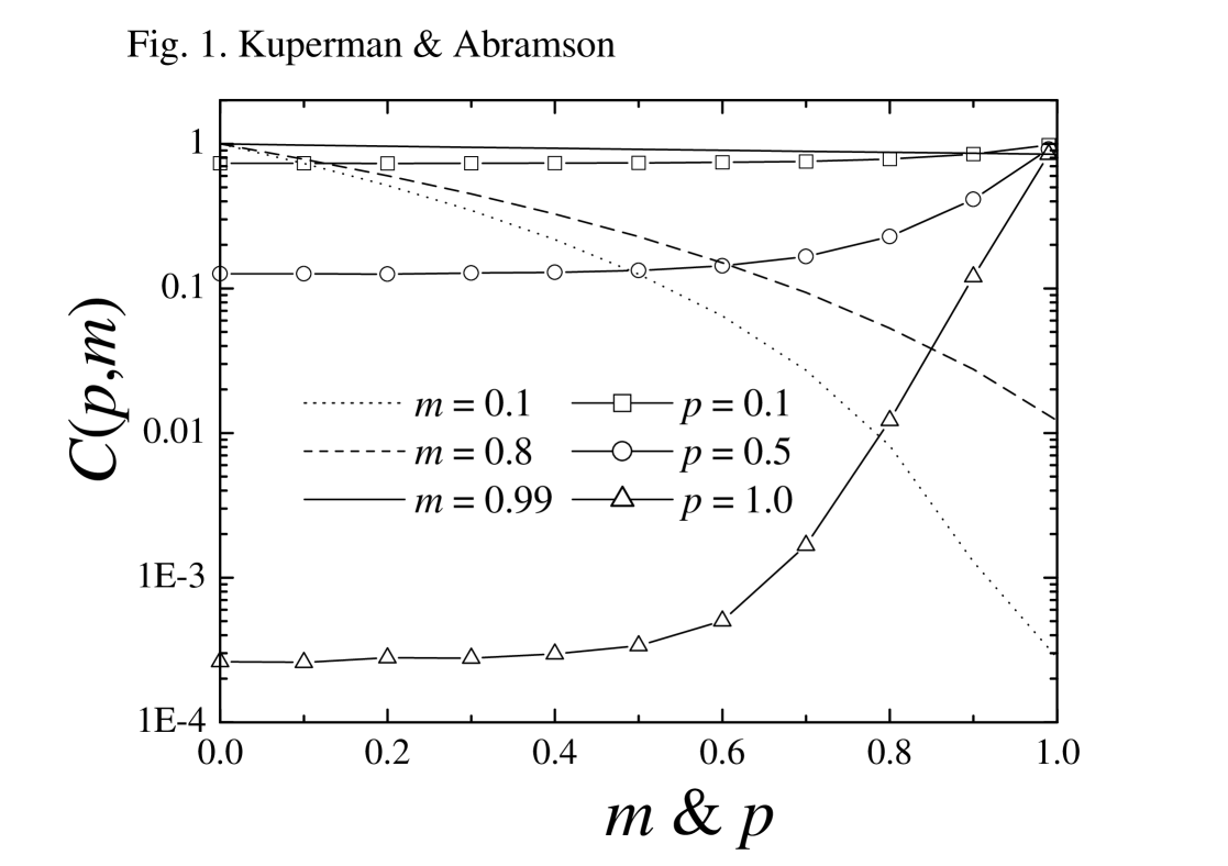
Figure 1: Average clusterization $C$ is displayed as a function of the rewiring probability $p$, and of the exponent $m$, in the same plot. Data are shown for three values of $p$ (lines and symbols), and for three values of $m$ (lines), as indicated in the legend. $N=10^{5},K=10$.

As an example of a generalization in the spirit of the previous paragraph, we introduce only one family of SW networks taking $\Theta\varpropto q^{-m}$, with $0<m<1$. The case $m=0$ gives a uniform $\Theta(q)$ and is equivalent to already known cases. For $m\geq 1$ a non integrable divergence at $q=0$ limits the possibility of having a normalized probability distribution. Lets start with the study of the average clusterization $C(p,m)$. In Fig. 1, we show two groups of curves. $C(p,m)$ as a function of the rewiring parameter $p$ for three $m$ values is shown with lines. $C(p,m)$ as a function of $m$ for three values of $p$ is shown with lines and symbols. The system under study has $N=10^{5}$ elements and $K=10$. We can see that as $m$ increases the region of high clusterization moves toward higher values of $p$. This means that the region in the $0\leq p\leq 1$ interval where SW networks can be found is enlarged. The are other relevant aspect derived from this fact that will be analyzed later. This effect is much more evident in the second group of curves, $C(p,m)$ vs $m$. Moving along one of the curves, which means fixing a value of $p$, for example $p=0.5$ (circles) we can go from low clusterization at $m\approx 0$ (uniform distribution $\Theta$) to high clusterization as $m$ grows. All the curves converge to the maximum clusterization when $m$ approaches 1.

The other aspect of interest to be discussed is related to the internal structure of the resulting networks. In recent papers ama ; albe , it has been reported that different kinds of behavior can be found in the accumulated connectivity distribution of evolving networks. In the present model, as in Strogatz and Watts’, the connectivity presents a well defined mean value, and an exponential decay at high values. This difference is a consequence of the construction method. At the same time, there is an interesting correlation between local clusterization and connectivity values that is worth analyzing. In Fig. 2 we show a plot of the connectivity vs. the clusterization of each element in the system. It can be observed that for each value of the connectivity there are elements with widely different clusterization. This shows that a characterization of this kind of networks in terms of the connectivity alone is incomplete. It is remarkable that, at low values of $p$, for each value of the connectivity, all (or almost all) the allowed values of $C$ are present in the system. In contrast, at high values of $p$, an emerging structure can be observed. The elements fall into classes of clusterization. Each class is characterized by a scale free relationship between connectivity and clusterization. This is apparent in Fig. 2.b), where each class is represented by the dots falling on straight lines in the log-log plot. In both plots, the occupied region is upper bounded by an envelope with power law decay. That is, highly connected elements are restricted to a range of low clusterizations, while lowly connected elements are responsible for the preservation of the high clusterization of the network. In qualitative terms we see that the network is partitioned into small subnetworks composed mainly by elements of low connectivity, while the long distance connection between each subunit is accomplished by highly connected (popular but otherwise lowly clustered) elements.

When analyzing internally the structures of the obtained networks we can see that several kinds of small world structures can arise. An example for small systems ($N=30,K=2$) and two kind of structures is shown in Fig. 3. Both correspond to the same value of the rewiring parameter $p=0.5$, meaning that approximately one half of the links have been reconnected. In Fig. 3.b) we can see an organization of the links in two levels: part of the rewired links have formed local subnetworks of high clusterization, while some others are connecting these structures between them. This is due to the fact that the distribution $\Theta=q^{-0.9}$ favors links to near vertices. In Fig. 3.a), instead, $\Theta$ is uniform, there is no preference in the reconnection process, and no local structures are formed. Case (b) could, at first sight, be confused with an $m=0$ network with a value of $p$ significantly lower than the current 0.5. However, in that case, much less links would have been rewired. The average clusterization would be around 0.5 instead of 0.4. In a system with significantly greater $N$ and $K$, one would expect a hierarchical organization in the connectivity of subnetworks. This organization can be controlled by the election of the distribution $\Theta$.

Let us now turn to the distribution of the clusterization in the system. In Fig. 4 we show histograms of the values of the individual clusterization in the system, for four selected values of $m$ and $p$. Each value of the local clusterization present in the system (a discrete magnitude) is represented by a dot, at a height proportional to its frequency. We can observe the incidence of the parameters into the internal organization of the clusterization of the network. The effect of the rewiring $p$ is different at different values of $m$. It is interesting to observe that each distribution is composed by a superposition of many branches. Each one of these comprises a number of elements of nearby clusterization.

We calculate now the cumulative probability distribution of clusterization $Q(C)=\sum_{C}^{1}P(C^{\prime})$, that represents the probability that an element has clusterization $C$ or greater. In figures 5 and 6 we show the accumulated clusterization $Q(C)$ for three values of the rewiring parameter $p$. Fig. 5 corresponds to a slightly non uniform distribution $\Theta=q^{-0.1}$ while Fig. 6 corresponds to a highly non uniform distribution $\Theta=q^{-0.99}$. First, observe (in any of the figures) that different values of $p$ produce different behaviors in the accumulated distribution. In Fig. 5 we have $m=0.1$. This slight departure from the uniformity (Strogatz and Watts’ model) produces a slower decay of $Q$ for growing $p$, appreciable as a change of the curvature in the log plots. The fact that $\Theta=q^{-0.99}$ generates networks with many highly clustered elements (independently of $p$) can be seen in Fig. 6 as a plateau that reaches high values of $C$. Even if the three distributions in Fig. 6 decay in similar way, they arise from distributions $P(C)$ as differing as those shown in Fig. 4 (bottom row). Note also in Figs. 5 and 6 that the effect of a $\Theta$ that favors high clusterization can be seen even at low levels of disorder as $p=0.1$. This can be appreciated by comparing the curves corresponding to $p=0.1$ in Figs. 5 and 6 (full lines), where the plateau in $Q(C)$ shows that almost all the values of clusterization are above $0.4$ in the first case, and above $0.7$ in the second.

We have used $\Theta=q^{-m}$ as an example of a distribution used to generate the rewiring. The present scheme is rather flexible to produce a variety of clusterization distributions and topologies, through the election of a proper distribution $\Theta$. This fact may be relevant in the modelling of real networks. At the present time several social phenomena have been modelled on the basis of a SW network abra ; kup ; pastor .

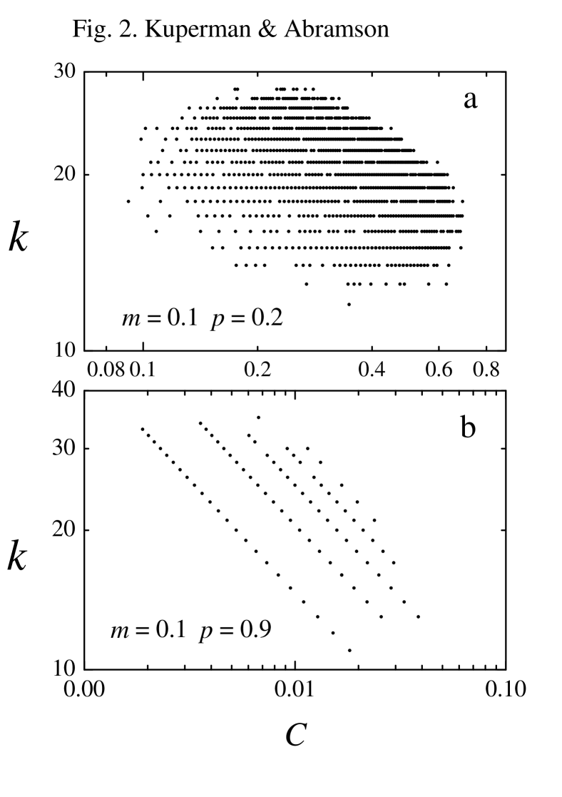
Figure 2: Connectivity vs clusterization for each element in the system. (a) $m=0.1$, $p=0.2$. (b) $m=0.1$, $p=0.9$. In both plots, $N=10^{5},K=10$. Except points with $c=0$ (not shown for reasons of scale), all points are plotted.

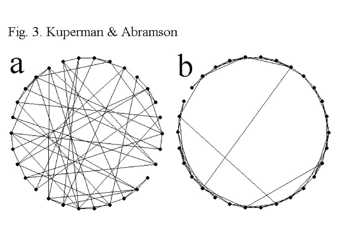
Figure 3: Two small worlds with 30 elements and $K=2$. They have the same degree of rewiring but differing distribution $\Theta$. (a) $p=0.5$, $m=0$. $C=0.11$ (b) $p=0.5$, $m=0.9$. $C=0.41$.

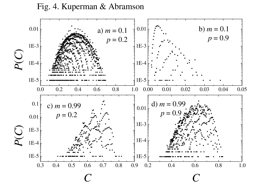
Figure 4: Distribution of the local clusterization. Values of $m$ and $p$ as indicated in the legends. In all plots, $N=10^{5},K=10$. Except points with $c=0$ (not shown for reasons of scale), all points are plotted.

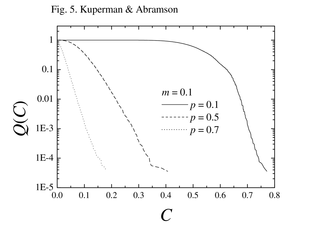
Figure 5: Accumulated probability of finding an element with clusterization $C$ or more. Data are shown for $m=0.1$, and three values of $p$, as indicated in the legend. $N=10^{5}$ and $K=10$.

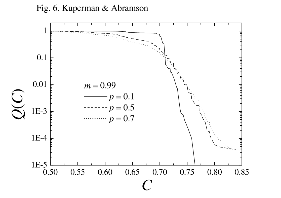
Figure 6: Accumulated probability of finding an element with clusterization $C$ or more. Data are shown for $m=0.99$, and three values of $p$, as indicated in the legend. $N=10^{5}$ and $K=10$.

References

- (1) S. Milgram, Psychol. Today 2, 60-67 (1967)
- (2) D. J. Watts and S. H. Strogatz, Nature 393, 440–442 (1998).
- (3) D. J. Watts, Small Worlds (Princeton University Press, 1999).
- (4) L. A. N. Amaral, A. Scala, M. Barthélemy and H. E. Stanley, Proc. Natl. Acad. Sci. U.S.A. 97, 11149 (2000).
- (5) R. Albert and A.L. Barabási, Phys. Rev. Lett. 85, 5234 (2000)
- (6) G. Abramson and M. Kuperman, Phys. Rev. E. 63 030901(R) (2001).
- (7) M. Kuperman and G. Abramson, Phys. Rev. Lett. (2001, in the press).
- (8) Romualdo Pastor-Satorras and A. Vespignani, preprint cond-mat/0102028.