Measures of Anisotropy and the Universal Properties of Turbulence

Abstract

Local isotropy, or the statistical isotropy of small scales, is one of the basic assumptions underlying Kolmogorov’s theory of universality of small-scale turbulent motion. The literature is replete with studies purporting to examine its validity and limitations. While, until the mid-seventies or so, local isotropy was accepted as a plausible approximation at high enough Reynolds numbers, various empirical observations that have accumulated since then suggest that local isotropy may not obtain at any Reynolds number. This throws doubt on the existence of universal aspects of turbulence. Part of the problem in refining this loose statement is the absence until now of serious efforts to separate the isotropic component of any statistical object from its anisotropic components. These notes examine in some detail the isotropic and anisotropic contributions to structure functions by considering their SO(3) decomposition. After an initial discussion of the status of local isotropy (section 1) and the theoretical background for the SO(3) decomposition (section 2), we provide an account of the experimental data (section 3) and their analysis (sections 4, 5 and 6). Viewed in terms of the relative importance of the isotropic part to the anisotropic parts of structure functions, the basic conclusion is that the isotropic part dominates the small scales at least up to order 6. This follows from the fact that, at least up to that order, there exists a hierarchy of increasingly larger power-law exponents, corresponding to increasingly higher-order anisotropic sectors of the SO(3) decomposition. The numerical values of the exponents deduced from experiment suggest that the anisotropic parts in each order roll off less sharply than previously thought by dimensional considerations, but they do so nevertheless.

1 Introduction

Local isotropy, or the isotropy of small scales of turbulent motion, is one of the assumptions at the core of the belief that small scales attain some semblance of universality [11]. This is a statistical concept, and is not necessarily opposed to the idea of structured geometry of small scales [9]. The important question about local isotropy is not whether the small scales are strictly isotropic, but the degree to which the notion becomes a better approximation as the scales become smaller [20]. Aside from the generic requirement that the flow Reynolds number be high (so that small scales as a distinct range may exist independent of the large scale), the question of how or if local isotropy becomes a good working approximation depends on the nature of large-scale anisotropy, on whether or not there are other body forces, on the nearness to physical boundaries, etc. All of this was well understood by the time of publication of Monin & Yaglom [19]. The general consensus at the time seems to have been that small scales indeed attain isotropy far from the boundary at high enough Reynolds numbers, at least when one considered second-order quantities.

The situation changed perceptibly when the small scales of scalar fluctuations were experimentally found to be anisotropic in many types of shear flows even at the highest Reynolds numbers of measurement. For a summary, see Ref. [23]. Since that time, various other pieces of evidence are slowly accumulating to suggest that small-scale velocity is also anisotropic; see, for example, Ref. [22]. The claim is that the previously held belief—which, to some degree, was comforting—loomed large only because we had not explored the right statistical quantities. The notion that anisotropy persists at all scales at all Reynolds numbers (though manifested only in certain statistical parameters) puts a strong damper on any theory that purports to consider small-scale turbulence as a universal object. This is somewhat of an impasse.

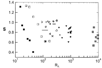
Figure 1: The magnitude of the skewness of the temperature derivative in turbulent shear flows. The figure is taken from Ref. [24]. The Taylor microscale Reynolds number $R_{\lambda}$ is proportional to the square root of the large scale Reynolds number. It is defined more precisely in section 2.

Since the problems began with passive scalars, we might as well consider the evidence in that case a little more closely. The evidence, collected over many years by many people, is reproduced in Fig. 1 from Ref. [24]. The argument is that if the temperature fluctuation $\theta$ is locally isotropic, its derivative $\partial\theta/\partial x$, being a small-scale quantity by construction, should be isotropic. Taking reflection symmetry as part of isotropy, we should have $\langle(\partial\theta/\partial x)^{n}\rangle$ = $-\langle(\partial\theta/\partial x)^{n}\rangle$ for all odd values of $n$. This means that all the odd moments must be zero. In particular, $\langle(\partial\theta/\partial x)^{3}\rangle=0$, or ‘small’ in practice. But small compared to what? The standard thing to do is to normalize $\langle(\partial\theta/\partial x)^{3}\rangle$ by $\langle(\partial\theta/\partial x)^{2}\rangle^{3/2}$, or to examine the behavior of the skewness $S$ of $\partial\theta/\partial x$. These are the data shown in Fig. 1. The data suggest, despite some large scatter, that the skewness remains to be of the order unity even at the largest Reynolds numbers for which measurements are available.

There are two points to be made. The first is that the Taylor microscale Reynolds number $R_{\lambda}$ may not be the right parameter against which to plot $S$. As articulated by Hill [8], the reasons are that the velocity that appears in $R_{\lambda}$ is a large-scale quantity and the length scale $\lambda$ cannot be defined independent of the large scale velocity. (In practice, the definition of $\lambda$ may not require the large scale, see [26], though this is not a result that can be shown formally; but the comment on the velocity remains valid in any case.) We believe, however, that the situation will probably not change qualitatively even if we adopted a different abscissae for Fig. 1. The second point is that, if one used $\langle(\partial\theta/\partial x)^{4}\rangle^{3/4}$ instead of $\langle(\partial\theta/\partial x)^{2}\rangle^{3/2}$ for normalizing $\langle(\partial\theta/\partial x)^{3}\rangle$, the normalized quantity will vanish with Reynolds number, roughly according to some power of the Reynolds number. Why is it not legitimate to compare the third moment to the next high-order even moment, instead of the neighboring low-order moment, or, perhaps to the geometric mean of the lower and higher order even moments? In either case, we will have a quantity that diminishes with the Reynolds number.

These are not elegant arguments, and seem like desperate efforts made to save the situation at any cost. There is a further argument to be made, however. Leaving aside the technicalities for a moment, let us suppose that, for a given statistical quantity to be measured, there are at all scales an isotropic part and an anisotropic part. We might now ask whether the ratio of the anisotropic part to the isotropic part vanishes as the scale size becomes smaller. We are no longer asking if the third moment vanishes with respect to (a suitable power of) some even order moment, but if, within a moment of a given order, the isotropic part eventually dominates the anisotropic part as the scale size vanishes. If this is indeed so, it allows us to say that, while non-universal anisotropic parts may always be present, the isotropic part dominates at small enough scales. If, of course, the isotropic part contributes exactly zero to the statistical quantity being considered, the anisotropic part will no doubt prevail at any finite Reynolds number, but this is not in contradiction to the statement just made. This is a richer point of view to take, potentially less inhibiting for the development of a sensible theory of turbulence. In such a picture, the universal theory that may emerge holds for the isotropic part alone, but, for it to be applicable to other types of turbulence, the anisotropic ‘correction’ has to be added in some suitable way.

The questions of interest, then, are obvious: What is a good way to decompose any statistical object of choice into isotropic and anisotropic parts? How do these two parts vary with scale size, relative to each other? A plausible method for answering these questions was proposed in Ref. [5] by using the SO(3) decomposition of tensorial objects usually considered in turbulence. One can argue as to whether this is the best perspective, but there is no doubt that it provides one framework within which our questions can be posed and answered. An experimental assessment of this issue is the broad topic of these notes. This is preceded by a detailed description of the theoretical issues involved.

The notes were part of the lectures presented by KRS at Les Houches, and form part of the Ph.D. work of SK. We note in advance that the literature cited is limited to a few key articles. We thank Itamar Procaccia and Victor L’vov for introducing us to the subject discussed here, and Christopher White and Brindesh Dhruva for their help in acquiring some of the data. KRS thanks the organizers of the School for the invitation to deliver the lectures.

2 Theoretical tools

2.1 The method of SO(3) decomposition

A familiar example of decomposition into the irreducible representations of the SO(3) symmetry group is the solution of the Laplace equation in spherical coordinates

$$\nabla^{2}{\psi}({\bf r})=0,$$ (1)

where ${\psi}$ is a scalar function defined over the sphere of radius $r$. This equation is linear, homogeneous and isotropic. The solutions are separable, and may be written as products of functions of $r$, $\theta$ and $\phi$. The solutions form a linear space, a possible basis for which are derived from the spherical harmonics $Y_{lm}(\theta,\phi)$

$$\psi_{lm}({\bf r})=r^{l}Y_{lm}(\theta,\phi)=r^{l}Y_{lm}({\bf{\hat{r}}})$$ (2)

where the index $l=0,1,2,...,\infty$ denotes the degree of the harmonic polynomial. The angular dependence ($\theta,\phi$) is equivalent to the unit vector ${\bf{\hat{r}}}$, or the unit sphere. In the angular dependence, the index $m$ denotes the elements of the orthonormal basis space that span each harmonic polynomial of degree $l$. For each $l$ there are $2l+1$ elements indexed by $m=-j,-j+1,\dots,j$ which are the $Y_{lm}$. Equation (2) is a useful basis space of solutions to the Laplace equation because the $\psi_{lm}({\bf{\hat{r}}})$ are each solutions of the Laplace equation and are orthonormal for different $l$,$m$. Each basis element has a definite behavior under rotations, that is, the action on it by an element of SO(3) preserves the indices. In other words, the rotated basis element will also be indexed by the same $l$,$m$. The general solution of (1) is given by

$$\psi({\bf r})=\sum_{l,m}a_{lm}\psi_{lm}({\bf r}).$$ (3)

The coefficients $a_{lm}$ are obtained from the boundary conditions on $\psi({\bf r})$ and, for a particular solution, any of them may be zero. In the theory of group representations, $\psi_{lm}({\bf r})$ is said to be the $2l+1$ dimensional irreducible representation of the group of all rotations, the SO(3) symmetry group, in the space of scalar functions over the sphere. The space of scalar functions is called a ‘carrier’ or ‘target’ space for the SO(3) group representations. For each irreducible representation indexed by $l=0...\infty$ there are $2l+1$ components indexed by $m=-l...+l$. A representation of a symmetry group is said to be irreducible if it does not contain any subspaces that are invariant under the transformation associated with that symmetry.

Here we make a distinction between the behaviors under rotation of the equation (1) and of its solutions $\psi({\bf r})$. The statement that the equation is isotropic means that it will hold true in a rotated frame with the Laplacian operator ${\overline{\nabla}}$ and the function ${\overline{\psi}}({\overline{\bf r}})$ properly defined in the new coordinate system, ${\overline{\nabla}}^{2}{\overline{\psi}}({\overline{\bf r}})=0$. However, the function $\psi({\bf r})$ may contain both isotropic and anisotropic components. All symmetry groups possess a one-dimensional representation in the carrier space, which is invariant under the transformations of that group. For the representations of the SO(3) symmetry group in the space of scalar functions over the unit sphere, the one-dimensional representation, indexed by $l=0$, is $Y_{00}=constant$; it will clearly remain unchanged under proper rotations. This is the isotropic representation. The higher-dimensional representations $Y_{lm}$ (dimension $3,5,7,\dots$ corresponding to $l=1,2,3,\dots$) have functional forms in $\theta$ and $\phi$ which are altered under rotation even though the degree ($l$), and hence the dimensionality, of the representation is preserved. These are the anisotropic representations. We examine this point in more detail with further discussion of the simple example of the scalar functions $\psi$.

For a particular rotation $\Lambda$ in Euclidean space which tells us how to rotate a vector ${\bf x}$ into a new coordinate system where it is denoted by ${\bf{\overline{x}}}$,

$${\overline{x}}^{\alpha}=\Lambda^{\alpha}_{\beta}x^{\beta},$$ (4)

we can define an operator $O_{\Lambda}$ which tells us how to rotate the function $\psi({\bf r})$ to ${\overline{\psi}}({\bf{\overline{r}}})$. If the function $\psi({\bf r})$ is written in terms of a linear combination of its basis elements as in Eq. (3), then the rotation operation is written as

$${\overline{\psi}}({\bf{\overline{r}}}) = O_{\Lambda}\psi({\bf r})$$ (5)

$$= O_{\Lambda}\sum_{l,m}a_{lm}\psi_{lm}({\bf r})$$

$$= \sum_{l,m}O_{\Lambda}a_{lm}\psi_{lm}({\bf r}).$$

The $O_{\Lambda}$ for each $l$ representation is a $(2l+1)\times(2l+1)$ matrix denoted by $D^{(l)}_{m^{\prime},m}(\Lambda)$. The transformation is written as

$$O_{\Lambda}\psi_{lm}({\bf r}) = \sum_{m^{\prime}=-l}^{l}D^{(l)}_{m^{\prime},m}(\Lambda)\psi_{lm^{\prime}}({\bf r}).$$ (6)

Thus, when a rotation of the function $\psi({\bf r})$ into a new coordinate system is to be performed, the rotation matrices $D^{(j)}_{m,m^{\prime}}(\Lambda)$ are all that is needed in order to transform each of the irreducible representations of the SO(3) group that form the basis functions of $\psi({\bf r})$. As can be seen from Eq. (6), the $j=0$ (one-dimensional) irreducible representation is the one which is invariant to all rotations in that its functional form is always preserved. The $D^{(0)}(\Lambda)$ matrix is merely a number, independent of $\Lambda$, multiplying the $j=0$ representation. The $j=0$ irreducible representation is the isotropic component of the SO(3) decomposition. For all higher-order $j$’s the rotation preserves the dimension of the transformed component, i.e. the indices $j$ and $m$ are retained, but the functional form is altered. The $D^{(j)}(\Lambda)$ for $j>0$ are true $(2j+1)\times(2j+1)$ matrices that mix the various $m$ contributions of the original, unrotated basis.

The above simple example involved the case of a scalar function $\psi$ that depended on a single unit vector ${\bf{\hat{r}}}$. The method of SO(3) decomposition may be carried over to more complicated objects. The theory is given in detail in [5]. In general we can imagine an $n^{th}$ order tensor function which depends on $p$ unit vectors $T^{\alpha_{1}\alpha_{2}\dots\alpha_{n}}({\bf{\hat{r}_{1}}},{\bf{\hat{r}_{2}}},\dots{\bf{\hat{r}_{p}}})$ and is the solution to an isotropic equation. Then, the rules of SO(3) decomposition carry over in the following manner. The rotation operator $O_{\Lambda}$ is now defined through the relation

$${\overline{T}}^{\alpha_{1}\alpha_{2}\dots\alpha_{n}}({\overline{\bf{\hat{r}_{1}}}},{\overline{\bf{\hat{r}_{2}}}},...{\overline{\bf{\hat{r}_{p}}}})=O_{\Lambda}T^{\alpha_{1}\alpha_{2}\dots\alpha_{n}}({\bf{\hat{r}_{1}}},{\bf{\hat{r}_{2}}},\dots,{\bf{\hat{r}_{p}}})$$ (7)

$$= \Lambda^{\alpha_{1}}_{\beta_{1}}\Lambda^{\alpha_{2}}_{\beta_{2}}\dots\Lambda^{\alpha_{n}}_{\beta_{n}}T^{\beta_{1}\beta_{2}\dots\beta_{n}}(\Lambda^{-1}{\overline{\bf{\hat{r}_{1}}}},\Lambda^{-1}{\overline{\bf{\hat{r}_{2}}}},\dots,\Lambda^{-1}{\overline{\bf{\hat{r}_{p}}}}).$$

The tensor function $T$ may be written in terms of the irreducible representations of the SO(3) symmetry group. The basis elements are denoted by $B^{\alpha_{1}\alpha_{2}\dots\alpha_{n}}_{jm}({\bf{\hat{r}}})$ where the $j$ index plays the same role as the $l$ index in the example of the scalar function. The basis elements are more complicated than the $\psi_{lm}$ because the space of functions $T$ is the direct product of $n$ Euclidean three-dimensional vector spaces (manifest in the indices $\alpha_{1}\dots\alpha_{n}$) with $p$ infinite dimensional spaces of continuous single-variable functions over the unit sphere (the ${\bf{\hat{r}_{1}}}\dots{\bf{\hat{r}_{p}}}$). If the constituent spaces are also written in the SO(3) decomposition, the rules of angular momentum addition, familiar from quantum mechanics, may be used in taking the direct product. The three-dimensional Euclidean vector space is a $j=1$ space while each of the infinite-dimensional spaces functions over the unit sphere is the sum of the $j=0,j=1,\dots,j\rightarrow\infty$ irreducible representations of SO(3) (recall the above example of $\psi({\bf{\hat{r}}})$) with each $j$ representation appearing once.

In tensor product notation, the product space of two vector spaces $V_{1}$ and $V_{2}$ is denoted by $V_{1}\otimes V_{2}$. In the case of vector spaces in the SO(3) notation the spaces are named uniquely by their index $j$. Using tensor product notation, the $n$ three-dimensional Euclidean spaces form a space $1\otimes 1\otimes\dots\otimes 1$ ($n$ times). The tensor notation indicating a linear sum of tensors with SO(3) representation indices $j_{1}$ and $j_{2}$ is $j_{1}\oplus j_{2}$. Using this notation, each of the infinite dimensional spaces is $0\oplus 1\oplus 2\oplus\dots$. The direct product of $p$ of these is ($0\oplus 1\oplus 2\oplus\dots)\otimes(0\oplus 1\oplus 2\oplus\dots)\otimes\dots\otimes(0\oplus 1\oplus 2\oplus\dots)$ ($p$ times). Thus, the final product space for $B_{jm}({\bf{\hat{r}}})$ is written in tensor-product notation as $1\otimes 1\otimes\dots\otimes 1$ ($n$ times) $\otimes(0\oplus 1\oplus 2\oplus\dots)\otimes(0\oplus 1\oplus 2\oplus\dots)\dots(0\oplus 1\oplus 2\oplus\dots)$ ($p$ times). Now, the tensor product of spaces $j_{1}$ and $j_{2}$ will contain new spaces whose SO(3) indices are given in the following manner. We recall the rules of angular momentum addition familiar from quantum mechanics. The total angular momentum of an SO(3) representation space is given by its index $j$. The rules of angular momentum addition dictate how the product of two spaces of angular momentum (SO(3) index) $j_{1}$ and $j_{2}$ may be added and the possible $j$ indices of the resulting spaces,

$$j_{1}\otimes j_{2}=|j_{1}-j_{2}|\oplus\dots\oplus(j_{1}+j_{2}).$$ (8)

Equation (8) says that the direct product of two spaces each belonging to a particular $j$ will generate a sum of new spaces with only those $j$ indices allowed by the rule. The operations $\otimes$ and $\oplus$ are distributive like the corresponding arithmetic operators. For example

$$1\otimes 1 = 0\oplus 1\oplus 2$$

$$1\otimes 1\otimes 1 = (0\oplus 1\oplus 2)\otimes 1$$ (9)

$$= (0\otimes 1)\oplus(1\otimes 1)\oplus(2\otimes 1).$$

If we now apply the angular momentum addition rules (8) to each of the product terms on the right hand side of Eq. (9), we get

$$1\otimes 1\otimes 1 = 1\oplus 0\oplus 1\oplus 2\oplus 1\oplus 2\oplus 3$$ (10)

$$= 0\oplus(1\times 3)\oplus(2\times 2)\oplus 3.$$

When taking the product of more than two spaces, there will be several ways to arrive at a particular $j$ in the final product space. We see this in the final rearrangement of the right hand side of Eq. (10), where there is only one representation each of $j=0$ and $j=3$, but three of $j=1$ and two of $j=2$. Going back to our more complicated target space for the basis elements $B^{\alpha_{1}\alpha_{2}\dots\alpha_{n}}_{jm}({\bf{\hat{r}}})$, which is $1\otimes 1\otimes\dots\otimes 1$ ($n$ times) $\otimes(0\oplus 1\oplus 2\oplus\dots)\otimes(0\oplus 1\oplus 2\oplus\dots)\dots(0\oplus 1\oplus 2\oplus\dots)$ ($p$ times), we expect that there may be many ways to obtain a particular $j$ in the final product space. To indicate this, for each basis element we associate a further index $q$ giving $B_{qjm}({\bf{\hat{r}}})$. These are important when we start to actually calculate the basis elements. The machinery used is the Clebsch-Gordan method well-known in quantum mechanics and the reader is referred to [5] for the details. The tensor $T$ may also depend on vectors ${\bf r_{i}}$ with magnitudes $r_{i}$ but for each rotation operation $O_{\Lambda}$ these may be treated as parameters included in the weight associated with each basis element. The $T$ are represented as

$$T^{\alpha_{1}\alpha_{2}\dots\alpha_{n}}({\bf r_{1}},{\bf r_{2}},\dots,{\bf r_{p}})=\sum_{q,j,m}a_{qjm}(r_{1},r_{2},\dots,r_{p})$$

$$\times B^{\alpha_{1}\alpha_{2}\dots\alpha_{n}}_{qjm}({\bf{\hat{r}_{1}}},{\bf{\hat{r}_{2}}},\dots,{\bf{\hat{r}_{p}}}).$$ (11)

In the next two sections, we move away from the very general formalism of SO(3) decomposition discussed above, and apply it to the specific case of the statistical tensor quantities in fluid turbulence and their dynamical equations obtained from the Navier-Stokes equations. We are motivated by the observation that the SO(3) decomposition when applied in the correct manner would allow ($a$) separation of the scaling variable $r$ from the angular dependence, and ($b$) the separation of the isotropic from the anisotropic parts of the tensor.

2.2 Foliation of the structure function into $j$-sectors

We would like to use the formalism of the SO(3) representation, as presented in general terms in the previous section, to study the structure function tensor in turbulence theory. The $n$th order structure function is defined by an ensemble average of the $n$th moment of the difference of velocity components across scales $r_{p}$. It is in fact a tensor function over $p$ unit spheres. We define the velocity difference as

$$w^{\alpha_{i}}({\bf r_{k}})=u^{\alpha_{i}}({\bf x+r_{k}})-u^{\alpha_{i}}({\bf x}),$$ (12)

where the $\alpha_{i}$ denotes the component of the velocity vector in the direction $i$ in a defined coordinate system, and the subscript $k$ on ${\bf r_{k}}$ denotes a particular choice of the vector. The $n$th order structure function for $p$ such choices of vector scale ${\bf r}$ is then

$$S^{\alpha_{1}\alpha_{2}\dots\alpha_{n}}({\bf r_{1}},{\bf r_{2}},\dots,{\bf r_{p}})=\langle w^{\alpha_{1}}({\bf r_{i}})w^{\alpha_{2}}({\bf r_{j}})\dots\times w^{\alpha_{n}}({\bf r_{k}})\rangle,$$ (13)

where the subscripts $i$,$j$,$\dots$ denote any of the vectors from ${\bf r_{1}}$ to ${\bf r_{p}}$.

In this section we review briefly the reason why the structure functions may be written as a linear combination of the irreducible representations of the SO(3) symmetry group. For details the reader is again referred to [5]. The dynamical equation for the structure function may be derived from the Navier-Stokes equations. Similar to the solutions of the Laplace equation, the solution to the $n$th order structure function equation forms a linear space with the basis chosen to be the irreducible representations $B_{qjm}({\bf r})$ of the SO(3) group as shown in previous sections (see Eq. (11). Since the basis is orthonormal for different $j,m$, and the equation is isotropic, we obtain a $heirarchy$ of dynamical equations each with terms of a $given$ $j$ and $m$. This demonstrates that the dynamical equations themselves $do$ $not$ mix the various $j$ and $m$ contributions, and that the dynamical equation for the $isotropic$ part of the structure function is different from the dynamical equations for any of the higher $j$ contributions. Further, it may be shown from solvability conditions on this set of equations that the scaling part of the function changes between $j$-sectors while remaining the same within a $j$-sector, for different $m$. This motivates the postulate that the different $j$ sectors scale with exponents different from the $isotropic$ $\zeta_{n}$. We denote these by $\zeta^{(j)}_{n}$ where subscript $n$ indicates the rank of the tensor and superscript $(j)$ indicates the number of the irreducible representation. We will leave out the superscript in the case of $j=0$ since then we recover the known isotropic scaling exponent $\zeta_{n}$.

2.3 The velocity structure functions

In the previous section we provided a heuristic justification for the use of the SO(3) decomposition for this tensor using the fact that it is the solution of an isotropic equation. Now, we use the rules of SO(3) (see Eq. (11)) decomposition to write it as

$$S^{\alpha_{1}\alpha_{2}\dots\alpha_{n}}({\bf r_{1}},{\bf r_{2}},\dots,{\bf r_{p}}) = \sum_{q,j,m}a_{qjm}(r_{1},r_{2},\dots,r_{p})$$ (14)

$$\times B^{\alpha_{1}\alpha_{2}\dots\alpha_{n}}_{qjm}({\bf{\hat{r}_{1}}},{\bf{\hat{r}_{2}}},\dots,{\bf{\hat{r}_{p}}}).$$

In this form, as was demonstrated for the scalar function $\psi$, the $j=0$ representation is the isotropic one. Its prefactor $a_{q_{00}}(r_{1},r_{2},\dots,r_{p})$ contains the scale dependence. For $p>1$ there will be infinitely many ways to obtain a particular $j$ for the product space as may be seen from the angular momentum addition rules in Eq. (8) and the direct-product representation. Therefore, $q$ ranges from $1$ to $\infty$. This is a difficult hurdle computationally but, fortunately, most experimental and theoretical work deals with the dependence on a single vector, and $p=1$. In that case, and for rank $n=2$, we obtain the second order structure function $S^{\alpha\beta}({\bf r})$ quite easily.

2.3.1 The second-order structure function

We consider the structure function of Eq. (14) for $n=2$ and $p=1$. The tensor product space is

$$1\otimes 1\otimes(0\oplus 1\oplus 2\oplus\dots) = (0\oplus 1\oplus 2)\otimes(0\oplus 1\oplus 2\oplus\dots)$$ (15)

$$= (0\otimes 0)\oplus(0\otimes 1)\oplus(0\otimes 2)\oplus\dots$$

$$\oplus (1\otimes 0)\oplus(1\otimes 1)\oplus(1\otimes 2)\oplus\dots$$

$$\oplus (2\otimes 0)\oplus(2\otimes 1)\oplus(2\otimes 2)\oplus\dots.$$

As demonstrated in (10) using the addition rule (8), there could be more than one way of obtaining a particular $j$ representation is obtained in the product space. To count these for a given j, we had to add there the index $q$ to the basis tensors (see for example Eq. (11)). We find for the second-order tensor over a single sphere that

• $j=0$ has a total of 3 representations

• $j=1$ has a total of 7 representations

• $j>1$ has a total of 9 representations.

The Clebsch-Gordon machinery tells us in addition about the symmetry (in the indices) and parity (in $r$) of each $q$ contribution. Using this information, the terms of the basis may be constructed. As in the case of the scalar function, the $B^{\alpha\beta}_{qjm}$ are orthonormal for different $j$,$m$ and $q$. In practice, the Clebsch-Gordon method of constructing these objects is rather tedious and so we follow the alternative method offered in [5]. We make use of the Clebsch-Gordon methods only to obtain the number of representations in each $j$, and its parity and symmetry properties. Armed with this information, the $B^{\alpha\beta}_{qjm}$ may be constructed by a more convenient means. The idea is to use the fact that we already know an orthonormal basis in the SO(3) representation for the scalar function over the sphere (Eq. (2)). We can now ‘add indices’ to this basis in a way to be described, while retaining the properties under rotation, in other words its $j$ and $m$ values. To add indices in a way that does not change the $j$,$m$ values is to perform contraction with the objects $\delta^{\alpha\beta}$,$r^{\alpha}$,$\epsilon^{\alpha\beta\gamma}$ and the partial derivative operator $\partial_{\alpha}$. This method automatically takes care of the $j$ and $m$ properties; and all that needs to be done now is to apply the above operators to obtain the different $q$ terms with the right symmetry and parity properties. This gives us a complete set of basis elements which are different than the Clebsch-Gordan method. The orthonormality among different $q$ for the same $j$ and $m$ is lost, but the orthonormality among different $j$ and $m$ is maintained because we start out with a basis Eq. (2) which already possesses these properties. However, different $q$ elements are linearly independent and span a given ${j,m}$-sector. The details on how this is done using the rules from [5] is presented in appendix A. In what follows we simply write down the components calculated using that method.

The second order structure function tensor is

$$S^{\alpha\beta}({\bf r})=\langle(u^{\alpha}({\bf x+r})-u^{\alpha}({\bf x}))(u^{\beta}({\bf x+r})-u^{\beta}({\bf x}))\rangle$$ (16)

which we decompose using the SO(3) irreducible representations $B^{\alpha\beta}_{qjm}({\bf{\hat{r}}})$ as

$$S^{\alpha\beta}({\bf r}) = S^{\alpha\beta}_{j=0}({\bf r})+S^{\alpha\beta}_{j=1}({\bf r})+S^{\alpha\beta}_{j=2}({\bf r})+\dots$$ (17)

$$= \sum_{q,j,m}a_{qjm}(r)B^{\alpha\beta}_{qjm}(\alpha\beta)({\bf{\hat{r}}}).$$

A further constraint is provided by the incompressibility condition

$$\partial_{\alpha}S^{\alpha\beta}({\bf r})=0.$$ (18)

Each $j$,$m$-sector must separately satisfy the incompressibility condition since taking the partial derivative preserves the rotation properties and does not mix the $j,m$ sectors. Therefore, the incompressibility condition provides a constraint among the different $q$ contributions within a given $j,m$-sector. For example, the $j=0$ contribution has three different representations ($q=\{1,2,3\}$), two of which are symmetric and one antisymmetric in the indices $\alpha$, $\beta$. By definition, the structure function is symmetric in the indices, therefore the antisymmetric contribution will not appear giving only two $q$ contributions. The incompressibility constraint gives

$$\partial_{\alpha}\sum_{q}a_{q_{00}}r^{\zeta_{2}}B^{\alpha\beta}_{q_{00}}({\bf{\hat{r}}})=0,$$

and

$$\partial_{\alpha}(a_{100}r^{\zeta_{2}}\delta^{\alpha\beta}+a_{200}r^{\zeta_{2}}{r^{\alpha}r^{\beta}\over r^{2}})=0.$$ (20)

Motivated by the expectation that the structure functions scale as powers of $r$ in the inertial range, we assumed in Eq. (20) that the scale-dependent prefactor is of the form $a_{q_{00}}r^{\zeta_{n}}$ where $a_{q_{00}}$ is a flow-dependent constant. Equation (20) results in a relationship between $a_{100}$ and $a_{200}$ giving the final form of the isotropic $j=0$ sector with just one unknown coefficient $c_{0}$ to be determined by the flow boundary conditions. That is,

$$S^{\alpha\beta}_{j=0}({\bf r})=c_{0}r^{\zeta_{2}}\Big{[}(2+\zeta_{2})\delta^{\alpha\beta}-\zeta_{2}{r^{\alpha}r^{\beta}\over r^{2}}\Big{]}.$$ (21)

Here, $\zeta_{2}\approx 0.69$ is the known empirically known anomalous second-order scaling exponent. We would like to assume a similar scaling form for the prefactor $a_{qjm}(r)$ for $j>1$. In such a formulation, there is a hierarchy of scaling exponents which we denote by $\zeta^{(j)}_{2}\neq\zeta_{2}$ corresponding to the higher-order $j$ sectors. Successive $j$’s indicate increasing degrees of anisotropy. The following section provides a justification for such a classification of the scaling of the various sectors. It is the larger goal of this article to examine these aspects of the theory with the help of high-Reynolds-number data.

2.4 Dimensional estimates for the lowest order anisotropic scaling exponents

In this section we present dimensional considerations to determine the “classical” values expected for $\zeta_{2}^{(1)}$ and $\zeta_{2}^{(2)}$ the spirit of Kolmogorov’s 1941 theory (henceforth called K41). We work on the level of K41 to produce the value $\zeta_{2}^{(0)}=2/3$. Ignoring intermittency corrections is justified to the lowest order because the differences between any two values $\zeta_{2}^{(j)}$ and $\zeta_{2}^{(j^{\prime})}$ for $j\neq j^{\prime}$ are considerably larger than the intermittency corrections to either of them.

It is easiest to produce a dimensional estimate for $\zeta_{2}^{(2)}$. One simply asserts [15] that the $j=2$ contribution is the first one appearing in $S^{\alpha\beta}({\bf r})$ due to the existence of a shear. Since the shear is a second rank tensor, it can appear linearly in the $j=2$ contribution to $S^{\alpha\beta}({\bf r})$. We thus have for any $m$, $-j\leq m\leq j$,

$$S_{j=2}^{\alpha\beta}({\bf r})\sim T^{\alpha\beta\gamma\delta}{\partial\bar{U}^{\gamma}\over\partial r^{\delta}}f(r,\bar{\epsilon}).$$ (22)

Here $T^{\alpha\beta\gamma\delta}$ is a constant dimensionless tensor made of $\delta^{\alpha\beta}$, $\frac{r^{\alpha}}{r}$, and bilinear contributions made of the three unit vectors ${\hat{\bf p}},~{}{\hat{\bf m}},~{}{\hat{\bf n}}$, which form our coordinate system as defined in appendix A. The form of Eq. (22) means that the dimensional function $f(r,\bar{\epsilon})$ stands for the response of the second-order structure function to a small external shear. Within the K41 dimensional reasoning, this function in the inertial interval can be made only of the mean energy flux per unit time and mass, $\bar{\epsilon}$ and $r$ itself. The only combination of $\bar{\epsilon}$ and $r$ that yields the right dimensions of the function $f$ is $\bar{\epsilon}^{1/3}r^{4/3}$. Therefore

$$S_{j=2}^{\alpha\beta}({\bf r})\sim T^{\alpha\beta\gamma\delta}{\partial\bar{U}^{\gamma}\over\partial r^{\delta}}\bar{\epsilon}^{1/3}r^{4/3}\ .$$ (23)

We thus find a “classical K41” value of $\zeta_{2}^{(2)}$ to be $4/3$.

To obtain the value of $\zeta_{2}^{(1)}$ we cannot proceed in the same way. We need a contribution that is linear (rather than bilinear) in the unit vectors ${\hat{\bf p}},~{}{\hat{\bf m}},~{}{\hat{\bf n}}$. We cannot construct a contribution that is linear in the shear and yet does not vanish due to the incompressibility constraint. Thus there is a fundamental difference between the $j=2$ term and the $j=1$ term. While the former can be understood as an inhomogeneous term linear in the forced shear, the $j=1$ term, being more subtle, may perhaps be connected to a solution of some homogeneous equation well within the inertial interval.

We therefore need to consider some quantity other than the shear which could contribute to the anisotropy. One invariance in the inviscid limit is as given by Kelvin’s circulation theorem. In the so-called Clebsch representation, one writes the Euler equation in terms of one complex field $a({\bf r},t)$, see for example[16]. In the ${\bf k}$-representation, the Fourier component of the velocity field ${\bf u}({\bf k},t)$ is determined from a bilinear combination of the complex field

$${\bf u}({\bf k},t) = \frac{1}{8\pi^{3}}\int d^{3}k_{1}d^{3}k_{2}{\bf\Psi}({\bf k_{1}},{\bf k_{2}})a^{*}({\bf k_{1}},t)a({\bf k_{2}},t)\,$$ (24)

$${\bf\Psi}({\bf k_{1}},{\bf k_{2}}) = \frac{1}{2}\left({\bf k_{1}}+{\bf k_{2}}-({\bf k_{1}}-{\bf k_{2}})\frac{k_{1}^{2}-k_{2}^{2}}{|{\bf k_{1}}-{\bf k_{2}}|^{2}}\right).$$ (25)

It was argued in [16] that this representation reveals a local conserved integral of motion given by

$${\bf\Pi}=\frac{1}{8\pi^{3}}\int d^{3}k{\bf k}a^{*}({\bf k},t)a({\bf k},t).$$ (26)

Note that this conserved quantity is a vector, and so it cannot have a finite mean in an isotropic system. Consider a correction to the second order structure function due to a flux of the integral of motion $\bar{\bf\pi}$. The dimensionality of $\bar{\bf\pi}$ is $[\bar{\bf\pi}]=[\bar{\epsilon}^{2/3}/r^{1/3}]$, and therefore now the dimensionless factor is $\bar{\bf\pi}\,r^{1/3}/\bar{\epsilon}^{2/3}$. As we did with the shear in the case of the $j=2$, we assume here the expandability of $\delta_{\bf\pi}S$ at small values of the flux $\bar{\bf\pi}$ and find

$$S_{j=1}^{\alpha\beta}({\bf r})\sim T^{\alpha\beta\gamma}\,\bar{\pi}^{\gamma}\,r\,$$ (27)

where $T^{\alpha\beta\gamma}$ is a constant dimensionless tensor that is linear in the unit vectors $\hat{\bf p},~{}\hat{\bf m},~{}\hat{\bf n}$. We thus find the “classical K41” value $\zeta_{2}^{(1)}$ is $1$. The derivation of the exponents $\zeta_{2}^{(1)}$ and $\zeta_{2}^{(2)}$ is given in [12]. It is concluded that dimensional analysis predicts values of 2/3, 1 and 4/3 for $\zeta_{2}^{(j)}$ with $j=0$, 1 and 2 respectively. It is not known at present how to continue this line of argument for $j>2$.

For the higher-order structure functions $S^{\alpha_{1}\alpha_{2}\dots\alpha_{n}}({\bf r})$ where $n>2$, similar dimensional analysis may be performed in order to find the K41 contribution to scaling due to shear (corresponding to the $j=2$ component). For each $n$, the lowest order correction to scaling that is linear in the shear is $n/3+2/3$.

2.5 Summary

The technique of SO(3) decomposition may be used in order to write the structure function tensor in terms of its isotropic part, indexed by $j=0$, and higher-order anisotropic parts, indexed by $j>0$. The dynamical equation for the structure function of order $n$ foliates into a set of equations each of different $j,m$. This motivates the postulate that the different sectors scale differently. The theory also indicates that any scaling behavior would depend only the $j$ index and be independent of the $m$ within that sector. There is allowance for dependence on boundary conditions, specific kinds of forcing and so on, in the unknown coefficients $a_{qjm}$ in the SO(3) expansion (Eq. (11)). We first consider the second-order structure function in a detailed manner in the light of this group representation. The analysis may be implemented for structure functions of any order but the task becomes computationally and conceptually more difficult for $n>2$. In section 6, we present a means of circumventing these problems.

We have reviewed the theoretical estimates for the low-order anisotropic scaling exponents for the second-order structure function. The method may be carried over to the higher-order objects as well, and we have derived the lowest order shear-dependent scaling contributions to the $n^{th}$ order structure function to be $r^{n/3+2/3}$. For the second-order structure function, we have shown that the $j=2$ contribution corresponds to a low-order shear-dependency. Again for the second-order structure function, we have presented a conserved quantity in the Clebsch-representation which provides the correct dimensional properties for the $j=1$ scaling contribution to be $r$. The arguments used are purely dimensional in the K41 sense, and do not take account of anomalous scaling. We expect that real turbulent flows will exhibit anomalous scaling in the isotropic sector, $and$ in every anisotropic sector in the SO(3) hierarchy. The issue of anomalous exponents in turbulence has now multiplied several-fold, to all the $j$ sectors, in light of the apparent universality that this work suggests. Thus, the theoretically predicted anisotropic exponents are to be treated merely as estimates, especially for higher-order structure functions ($n>2$), since the scaling anomalies are expected to increase with the order $n$, similar to the isotropic case.

In subsequent sections we demonstrate the use of experimental data in order to test the predictions of the theory. In particular, we provide explicit calculations of measurable tensor quantities and extract scaling corrections due to anisotropy.

3 Some experimental considerations

3.1 Background

Experimental studies of turbulent flows at very high Reynolds numbers are usually limited in the sense that one measures the velocity field at a single spatial point, or a few spatial points, as a function of time [19], and uses Taylor’s hypothesis to identify velocity increments at different times with those across spatial length scales, $r$. The standard outputs of such single-point measurements are the longitudinal two-point differences of the Eulerian velocity field and their moments. In homogeneous and isotropic turbulence, these structure functions are observed to vary as power-laws in $r$, with scaling exponents $\zeta_{n}$ [7].

Recent progress in measurements and in simulations has begun to offer information about the tensorial nature of structure functions. Ideally, one would like to measure the tensorial $n$th order structure functions defined in Eqs. (12) and (13). Such information should be useful in studying the anisotropic effects induced by all practical means of forcing.

3.2 Relevance of the anisotropic contributions

In analyzing experimental data the model of “homogeneous and isotropic small-scale” is universally adopted, but it is important to examine the relevance of this model for realistic flows. As we will demonstrate in the next chapter, our data we use exhibit anisotropy down to fairly small scales [25]. We have shown mathematically that keeping the tensorial information helps significantly in disentangling different scaling contributions to structure functions. In the light of the SO(3) representation of section 2, where it is shown that anisotropy might lead to different scaling exponents for different tensorial components, a careful study of the various contributions is needed. This is our goal in the rest of this article.

3.3 The measurements

In order to extract a particular $j$ contribution and the associated scaling exponent, one would ideally like to possess the statistics of the velocity at all points in three-dimensional space. One could then extract the $j$ contribution of particular interest by multiplying the full structure function by the appropriate $B_{qjm}$ and integrating over a sphere of radius $r$. Orthogonality of the basis functions ensures that only the $j$ contribution survives the integration. One could then perform this procedure for various $r$ and extract the scaling behaviors.

The method just described was adopted successfully in [2] using data from direct numerical simulations of channel flows. The Taylor microscale Reynolds number $R_{\lambda}$ for the simulations was about 70. This is not large enough for a clear inertial scaling range to exist. The authors of Ref. [2] resort to extended self-similarity (ESS) in both the isotropic and the anisotropic sectors. Nonetheless, the results indicated a scaling exponent of about $4/3$ in the $j=2$ sector. While the experimental data are limited to a few points in space, and the integration over the sphere is not possible, we are able to attain very high Reynolds numbers especially in the atmosphere under steady conditions ($R_{\lambda}\approx 10,000-20,000$). Despite the advantage of extended scaling range, we are however faced with a true superposition of contributions from various $j$ sectors with no simple way of disentangling them as was done with the numerical data. However, as we will show in section 6, we can make a judicious choice of the tensor components studied, and obtain access to the anisotropic contributions.

The tensor structure of the velocity structure functions is lost in the computation of the usual single-point single-component measurement of longitudinal and transverse objects. This is because the part of the expansion that is dependent on the angle $\theta$ is hidden: the longitudinal and transverse components set the value of $\theta$ to a constant. The boundary-dependent prefactors now collapse to a single number as

$$S^{\alpha\beta}_{j=2}(r)=ar^{\zeta^{(j)}_{2}}.$$ (28)

On the one hand, this is a simple expression. On the other, the angular dependence is completely lost and there is no formal difference from the isotropic object

$$S^{\alpha\beta}_{j=0}(r)=c_{0}r^{\zeta_{2}}.$$ (29)

In order to see the true tensor character of the structure function we need an angular variation of the scale separation $r$. In the atmospheric boundary layer which offers the highest Reynolds numbers available, the simplest configuration that would allow us to do this is a two hot-wire combination separated by distance $\Delta$ in the spanwise direction (y), orthogonal to the mean-wind. By Taylor’s frozen flow hypothesis, such a set-up will provide two simultaneous one-dimensional cuts through the flow. Therefore, one can measure the correlation between the two probes, across a scale $r$ that makes an angle $\theta$ with the mean-wind direction. As $r$ varies, the angle with respect to the mean-wind will also vary, giving some functional dependence on $\theta$ for the coefficients in the SO(3) decomposition. A schematic of the experimental configuration is presented in Fig. 2.

Figure 2: Schematic of the experimental set-up. Shown is the positioning of the single wire probes 1 and 2 with respect to the mean wind, and a visual explanation of how Taylor’s hypothesis is employed. The coordinate system chosen is different from what is conventional in turbulence—where the mean-wind is taken to lie along the $x$-axis. The pictured choice of coordinates simplifies the calculations involving the spherical harmonics.

A final consideration in measurements aimed at measuring anisotropic contributions is the homogeneity of the flow. The incompressibility condition may only be applied as a constraint on the structure function coefficients if the flow is homogeneous in the $r$ direction. If we consider, for instance, probes separated in the shear (vertical) direction, $r$ will have a component in the inhomogeneous direction and incompressibility may not be used to constrain the terms in the S0(3) expansion, leaving too many free parameters. However, in some instances, it is important to consider quantities that are not constrained by the incompressibility condition. For example, the $j=1$ contribution to the second order structure function will not appear in the experimental configuration described above. This is so because only one symmetric, even-parity, term exists in $j=1$ by the Clebsch-Gordon rules, and this must vanish by the incompressibility constraint. Probe-separation in the shear direction would be needed to produce a non-zero contribution of the $j=1$ term. In short, one can understand the nature of the best experimental configuration from carefully studying the tensor decomposition of the structure function.

Height $\overline{U}$ $u^{\prime}$ $10^{2}\langle\varepsilon\rangle$, $\eta$ $\lambda$ $R_{\lambda}$ $f_{s},$ per # of meters ms^-1 ms ^-1 m ² s^-3 mm cm channel, Hz samples 6 4.1 1.08 $1.1$ 0.75 15 10,500 10,000 $4\times 10^{7}$ 35 8.3 2.30 $7.8$ 0.45 13 19,500 5,000 $4\times 10^{7}$ 0.11 2.7 0.47 $6.6$ 0.47 2.8 900 5,000 $8\times 10^{6}$ 0.27 3.1 0.48 2.8 0.6 4.4 1400 5,000 $8\times 10^{6}$ 0.54 3.5 0.5 1.5 0.7 6.2 2100 5,000 $8\times 10^{6}$

Table 1: Data sets I (first line), II (second line) and III (third-fifth lines). The various symbols have the following meanings: $\overline{U}$ = local mean velocity, $u^{\prime}$ = root-mean-square velocity, $\langle\varepsilon\rangle$ = energy dissipation rate obtained by the assumption of local isotropy and Taylor’s hypothesis, $\eta$ and $\lambda$ are the Kolmogorov and Taylor length scales, respectively, the microscale Reynolds number $R_{\lambda}\equiv u^{\prime}\lambda/\nu$, and $f_{s}$ is the sampling frequency.

We analyze measurements in atmospheric turbulence at various heights above the ground (data sets I, II and III). Sets I and III were acquired from flow over a long fetch in the salt flats in Utah. The site of measurements was chosen to provide steady wind conditions. The surface of the desert was smooth and even: the water that floods the land during spring recedes uniformly and leaves the ground hard and essentially smooth during early summer. The boundary layer on the desert floor in early summer is thus quite similar to that on a smooth flat plate [10]. The measurements were made in the early summer season roughly between 6 PM and 9 PM during which nearly neutral stability conditions prevailed. Data set II was acquired over a rough terrain with ill-defined fetch at the meteorological tower at the Brookhaven National Laboratory. In sets I and II, data were acquired at heights 6 m and 35 m respectively. They were recorded simultaneously from two single hot-wire probes separated in the spanwise direction $y$ by 55 cm and 40 cm respectively. In both cases, the separation distance was within the inertial range, and was set nominally orthogonal to the mean wind direction (see below). Set III was acquired from an array of three cross-wires, arranged above each other at heights 11 cm, 27 cm and 54 cm respectively. These measurements are thus much closer to the desert floor.

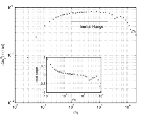
Figure 3: A typical compensated longitudinal third-order structure function. The inset indicates the region of isotropic inertial range scaling. (From Ref. [6].)

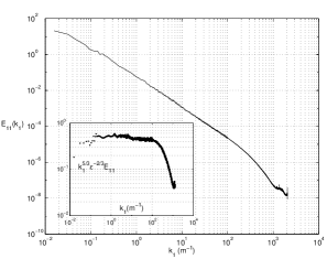
Figure 4: The one-dimensional energy spectrum computed from data set II. (From Ref. [6].)

The hot-wires, about 0.7 mm in length and 6 $\mu$m in diameter, were calibrated just prior to mounting them on the meteorology towers and checked immediately after dismounting. The hot-wires were operated on DISA 55M01 constant-temperature anemometers. The frequency response of the hot-wires was typically good up to 20 kHz. The voltages from the anemometers were suitably low-pass filtered and digitized. The voltages were constantly monitored on an oscilloscope to ensure that they did not exceed the digitizer limits. Also monitored on-line were power spectra from an HP 3561A Dynamic Signal Analyzer. The wind speed and direction were independently monitored by a direction indicator mounted on the tower (sets I and III), or a vane anemometer a few meters away (set II). The real-time durations of data records were limited only by the degree of constancy demanded of the wind speed and its direction.

The Taylor microscale Reynolds number was 10,000 for set I and about 20,000 for set II [6]. For set III, the corresponding numbers were 900, 1400 and 2100, respectively, at the three heights. Table 1 lists a few relevant facts about the data records analyzed here. Figure 3 shows a compensated third order longitudinal structure function and indicates the region over which the inertial range is expected to hold. As another example of the nature of the data, we show in Fig. 4 the longitudinal energy spectrum which displays extensive range of scaling. The slope is slightly larger than 5/3, as the compensated spectrum in the inset is supposed to clarify.

4 Anisotropic contribution in the case of homogeneity

4.1 General remarks on the data

We analyze data sets I and II described in section 3 (see Table 1) to extract the lowest order anisotropic contribution to scaling ([4],[12]). First, some preliminary tests and corrections need to be made. To test whether the separation between the two probes is indeed orthogonal to the mean wind, we computed the cross-correlation function $\langle u_{1}(t+\tau)u_{2}(t)\rangle$. Here, $u_{1}$ and $u_{2}$ refer to velocity fluctuations in the direction of the mean wind, for the arbitrarily numbered probes 1 and 2 respectively (see Fig. 2). If the separation were precisely orthogonal to the mean wind, the cross-correlation function should be maximum for $\tau=0$. Instead, for set I, we found the maximum shifted slightly to $\tau=0.022$ s, implying that the separation was not precisely orthogonal to the mean wind. To correct for this effect, the data from the second probe were time-shifted by 0.022 s. This amounts to a change in the actual value of the orthogonal distance. We computed this effective distance to be $\Delta\approx 54$ cm (instead of the 55 cm that was set physically). For set II, the effective separation distance was estimated to be 31 cm (instead of the physically set 40 cm). Next, we tested the isotropy of the flow for separations of the order of $\Delta$. Define the “transverse” structure function across $\Delta$ as $S_{T}(\Delta)\equiv\langle[u_{1}(\bar{U}t)-u_{2}(\bar{U}t)]^{2}\rangle$ and the “longitudinal” structure function as $S_{L}(\Delta)\equiv\langle[u_{1}(\bar{U}t+\bar{U}t_{\Delta})-u_{1}(\bar{U}t)]^{2}\rangle$ where $t_{\Delta}=\Delta/\bar{U}$. If the flow were isotropic we would expect [19]

$$S_{T}(\Delta)=S_{L}(\Delta)+{\Delta\over 2}{\partial S_{L}(\Delta)\over\partial\Delta}\ .$$ (30)

In the isotropic state both longitudinal and transverse components scale with the same exponent, $S_{T,L}(\Delta)\propto\Delta^{\zeta_{2}}$, and the ratio $S_{T}/S_{L}$ is computed from (30) to be $1+\zeta_{2}/2\approx 1.35$, because $\zeta_{2}\approx 0.69$ (see below). The experimental ratio was found to be 1.32 for set I, indicating that the anisotropy at the scale $\Delta$ is small. This same ratio was about 1.8 for set III, indicating higher degree of anisotropy in that scale range. The differences between the two data sets seem attributable partly to differences in the terrain and other atmospheric conditions, and partly to the different distances from the ground.

Lastly, we needed to assess the effects of high turbulence level on Taylor’s hypothesis. A comparison was made of the structure functions of two signals with turbulence levels differing by a factor of 2 and no difference was found. The correction scheme proposed in [27] also showed no changes. For a few separation distances, the statistics of velocity increments from two probes separated along ${\bf n}$, the direction of the mean wind, agreed with Taylor’s hypothesis. More details can be found in Ref. [6].

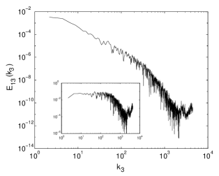
Figure 5: Log-log plot of the shear-stress cospectrum $E_{13}(k_{3})$ computed at 0.54 m. The inset shows a log-log plot of $k_{3}^{2.1}E_{13}(k_{3})$ vs. $k_{3}$. The flat region indicates a region of scaling with exponent -2.1.

The use of the isotropy equation (30) presents some evidence regarding the prevalence of modest amounts of anisotropy in the second-order statistics. This persistence is more explicit if one considers another familiar object, namely the cross-spectral density between horizontal and vertical velocity components. We consider the one-dimensional cross-spectral density (or shear-stress cospectrum) $E_{13}(k_{3})$, which is zero in the case of isotropy. From dimensional considerations, the scaling exponent for this quantity is $-7/3$ (see [15] for theory and [21] for experimental tests). Figure 5 shows the cospectrum computed for the height of 0.54 m. The inset shows that the cospectrum compensated with a scaling exponent of $-2.1$ is flat. To the extent that this is numerically smaller than 7/3, the decay of anisotropy is slower than expected for second-order quantities. Even allowing for the fact that the dimensional analysis assumes K41 scaling and therefore does not account for possible intermittency corrections in the anisotropic sectors, it is still clear that the small scales do not attain isotropy as fast as dimensional considerations suggest. We would like to use the properties of the SO(3) decomposition in order to disentangle the isotropic from the anisotropic contributions and better quantify the anisotropy. We first consider the second-order structure function in detail.

4.2 The tensor form for the second-order structure function

4.2.1 The anisotropic tensor component derived under the assumption of axisymmetry

To obtain a theoretical form of the structure function tensor we first select a natural coordinate system. Our choice is to have the mean-wind direction ${\bf n}$ along the z-axis which we label as 3. The angle with respect to the 3-axis is the polar angle $\theta$. The second axis is given by the separation vector ${\bf\Delta}$ between the two probes. We make the simplifying assumption that the main symmetry broken in the flow is the cylindrical symmetry about the mean-wind direction. In other words, the main anisotropic contribution is cylindrically symmetric about the mean-wind direction. It is shown a posteriori that this assumption probably accounts for most of the anisotropy for this particular geometrical set-up. In the next section, we provide a complete analysis with no assumptions about the symmetries of the flow. We conclude from that analysis that the simplification of the present section is not inconsistent with the properties of the full tensor.

Next, we write down the tensor form for the general second-order structure function (defined by Eq. (13) for $n=2$) in terms of irreducible representations of the SO(3) rotation group. Since we are far from the wall, our interest is in relatively modest anisotropies, and so we focus on the lowest order correction to the isotropic ($j=0$) contribution. We therefore write

$$S^{\alpha\beta}({\bf r})=S_{j=0}^{\alpha\beta}({\bf r})+S_{j=2}^{\alpha\beta}({\bf r})+\dots$$ (31)

We do not have a $j=1$ term because it vanishes from parity considerations (the structure function itself is even in $r$ in our experimental configuration) or by the incompressibility constraint. Assumed cylindrical symmetry of the anisotropic $j=2$ contribution implies that we only consider the $m=0$ subspace in this contribution. Now, the most general form of the tensor can be written down by inspection. The case $j=0$ is well known (see Eq. (21)) to be

$$S_{j=0}^{\alpha\beta}({\bf r})=c_{0}(r)\left[(2+\zeta_{2})\delta^{\alpha\beta}-\zeta_{2}{r^{\alpha}r^{\beta}\over r^{2}}\right]\,$$ (32)

where $c_{0}(r)=c_{0}r^{\zeta_{2}}$, and $c_{0}$ is a non-universal numerical coefficient that needs to be obtained from fits to the data. The $j=2$ component has six independent tensor forms and corresponding coefficients. These correspond to the different $a_{q_{00}}$ described in section 1. As with $j=0$, the $j=2$ component can be simplified by imposing conditions of incompressibility and orthogonality with the $j=0$ part of the tensor. This leaves us (in the case of cylindrical symmetry) with two independent coefficients which we call $a$ and $b$, giving,

$$S^{\alpha\beta}_{j=2}({\bf r}) = ar^{\zeta_{2}^{(2)}}\Big{[}(\zeta_{2}^{(2)}-2)\delta^{\alpha\beta}-\zeta_{2}^{(2)}(\zeta_{2}^{(2)}+6)$$

$$\times \delta^{\alpha\beta}{({\bf n}\cdot{\bf r})^{2}\over r^{2}}+2\zeta_{2}^{(2)}(\zeta_{2}^{(2)}-2){r^{\alpha}r^{\beta}({\bf n}\cdot{\bf r})^{2}\over r^{4}}$$

$$+ ([\zeta_{2}^{(2)}]^{2}+3\zeta_{2}^{(2)}+6)n^{\alpha}n^{\beta}$$

$$- {\zeta_{2}^{(2)}(\zeta_{2}^{(2)}-2)\over r^{2}}(r^{\alpha}n^{\beta}+r^{\beta}n^{\alpha})(\bf n\cdot\bf r)\Big{]}$$

$$+ br^{\zeta_{2}^{(2)}}\Big{[}-(\zeta_{2}^{(2)}+3)(\zeta_{2}^{(2)}+2)\delta^{\alpha\beta}(\bf n\cdot\bf r)^{2}$$

$$+ (\zeta_{2}^{(2)}-2){r^{\alpha}r^{\beta}\over r^{2}}+(\zeta_{2}^{(2)}+3)(\zeta_{2}^{(2)}+2)n^{\alpha}n^{\beta}$$

$$+ (2\zeta_{2}^{(2)}+1)(\zeta_{2}^{(2)}-2){{r^{\alpha}}{r^{\beta}}{({\bf n}\cdot{\bf r})^{2}}\over r^{4}}$$

$$- ([\zeta_{2}^{(2)}]^{2}-4)(r^{\alpha}n^{\beta}+r^{\beta}n^{\alpha})(\bf n\cdot\bf r)\Big{]}.$$

We note that the forms for the tensor were derived on the basis of the assumption of cylindrical symmetry. We used neither the Clebsch-Gordon method nor the “adding indices” method of section 1. This is why they were not automatically orthogonal to the $j=0$ contribution; that condition had to be explicitly imposed. However, in the end, this method also yields the same number of independent coefficients as the formal Clebsch-Gordon methods. This merely shows that there are different ways of writing the tensor forms for the basis elements. However, the Clebsch-Gordon rules tell us the number, parity and symmetry of the terms we must in the end have for a given $j,m$ sector.

Finally, we note that in the present experimental set-up only the component of the velocity in the direction of ${\bf n}$ (the 3-axis) is measured. In the coordinate system chosen above we can read from Eqs. (21) and (4.2.1) the relevant component to be

$$S^{33}(r,\theta) = S^{33}_{j=0}(r,\theta)+S^{33}_{j=2}(r,\theta)$$

$$= c_{0}\left({r\over\Delta}\right)^{\zeta_{2}}\Big{[}2+\zeta_{2}-\zeta_{2}\cos^{2}\theta\Big{]}$$

$$+ a\left({r\over\Delta}\right)^{\zeta_{2}^{(2)}}\Big{[}(\zeta_{2}^{(2)}+2)^{2}-\zeta_{2}^{(2)}(3\zeta_{2}^{(2)}+2)\cos^{2}\theta$$

$$+ 2\zeta_{2}^{(2)}(\zeta_{2}^{(2)}-2)\cos^{4}\theta\Big{]}$$

$$+ b\left({r\over\Delta}\right)^{\zeta_{2}^{(2)}}\Big{[}(\zeta_{2}^{(2)}+2)(\zeta_{2}^{(2)}+3)-\zeta_{2}^{(2)}(3\zeta_{2}^{(2)}+4)$$

$$\times \cos^{2}\theta+(2\zeta_{2}^{(2)}+1)(\zeta_{2}^{(2)}-2)\cos^{4}\theta\Big{]}\ .$$

Here $\theta$ is the angle between ${\bf r}$ and ${\bf n}$, and $r$ has been normalized by $\Delta$, making all the coefficients dimensional, with units of (m/sec)². Taylor’s hypothesis allows us to obtain components of $S^{\alpha\beta}$ from (4.2.1), with $\theta=0$ and variable, respectively. In other words,

$$S^{33}(r,\theta=0)=\langle[u_{1}(\bar{U}t+\bar{U}t_{r})-u_{1}(\bar{U}t)]^{2}\rangle\ ,$$ (35)

where $t_{r}\equiv r/\bar{U}$, and

$$S^{33}(r,\theta)=\langle[u_{1}(\bar{U}t+\bar{U}t_{\tilde{r}})-u_{2}(\bar{U}t)]^{2}\rangle.$$ (36)

Here $\theta=\arctan(\Delta/\bar{U}t_{\tilde{r}})$, $t_{\tilde{r}}=\tilde{r}/\bar{U}$, and $r=\sqrt{\Delta^{2}+(\bar{U}t_{\tilde{r}})^{2}}$.

The quantities on the left hand side of Eqs. (35) and (36) were computed from the experimental data and fitted to the theoretical expression (4.2.1) using the appropriate values of $\theta$. The fits were performed in the range $1<r/\Delta<10$ ($0.54$ m $<r<5.4$ m) for set I and $1<r/\Delta<25$ ($0.31$ m $<r<8$ m) for set II. The ranges were based on the constancy of the third order structure function (see Fig. 3 for an example). Panels (a) of Figs. 6 and 7 show, for data sets I and II respectively, a comparison between the measured $S^{33}(r,\theta=0)$ and the $j=0$ form of the equation. The comparison shows that the agreement is modest, and that the best-fit yields the exponent $\zeta_{2}$ to be $0.69$. A careful analysis of the data elsewhere [25] shows that, if the effect of the shear is removed in a plausible way, the power-law fit is excellent over a range of scale separations. To include the $j=2$ contribution, we fixed $\zeta_{2}$ to be 0.69 and performed the following analysis. For given values of the variables $r$ and $\theta$, we guessed the second exponent $\zeta_{2}^{(2)}$ and estimated the unknown coefficients $c_{0}$, $a$ and $b$ by using a linear regression algorithm. We followed this procedure repeatedly for different values of $\zeta_{2}^{(2)}$ ranging from $0$ to $2$. We then chose the value of $\zeta_{2}^{(2)}$ that minimized $\chi^{2}$ (the sum of the squares of the differences between the experimental data and the fitted values).

In Fig. 8 we present $\chi^{2}$ values as a function of $\zeta_{2}^{(2)}$. The optimal value of this exponent and the uncertainty determined from these plots is $\zeta_{2}^{(2)}\approx 1.38\pm 0.15$ from set I, and $\zeta_{2}^{(2)}\approx 1.36\pm 0.1$ from set II. The best numerical values for the coefficients are presented in Table 2. Panels (b) in Figs. 6 and 7 show fits to the sum of the $j=0$ and $j=2$ contributions to the experimental data. Even though the $j=2$ contributions are small, they improve the fits tremendously. This situation lends support to the essential correctness of the present analysis.

$\zeta_{2}$ $\zeta_{2}^{(2)}$ $c_{0}$ $a$ $b$ 0.69 1.38$\pm 0.15$ 0.023$\pm 0.001$ -0.0051$\pm 0.0006$ 0.0033$\pm 0.0005$ 0.69 1.36$\pm 0.10$ 0.112$\pm 0.001$ -0.052$\pm 0.004$ 0.050$\pm 0.004$

Table 2: The scaling exponents and the three coefficients in units of (m/sec)² as determined from the nonlinear fit of Eq. (7) to data sets I (first line) and II (second line).

Figure 6: The structure functions $S^{33}$ for $\theta=0$ and for non-zero $\theta$ computed for set I. The dots are for experimental data and the line is the analytic fit. Panel (a) presents fits to the $j=0$ component only, and panel (b) to components $j=0$ and $j=2$ together.

Figure 7: The structure functions $S^{33}$ for $\theta=0$ and for non-zero $\theta$ computed for set III. The dots are for experimental data and the line is the analytic fit. Panel (a) presents fits to the $j=0$ component only, and panel (b) to the sum of the components $j=0$ and $j=2$.

The figures show that the purely longitudinal structure function corresponding to $\theta=0$ is somewhat less affected by the anisotropy than is the finite $\theta$ structure function (see especially, Fig. 7). The reason is the closeness of the numerical absolute values of the coefficients $a$ and $b$ (see Table 2). For $\theta=0$ the two tensor forms multiplied by $a$ and $b$ coincide, and the $j=2$ contribution becomes very small. The value of $\zeta_{2}=0.69$ quoted above can be obtained from such a fit to the $\zeta_{2}=0$ part alone; as long as one measures only this component, it seems reasonable to proceed with just that one exponent. However, the inclusion of the second exponent $\zeta_{2}^{(2)}$ improves the fit even for the longitudinal case; for the finite $\theta$ case, this inclusion appears essential for a good fit. In fact, the fit using $j=0$ and $j=2$ for data set II extends all the way to 40 m (beyond the range shown in Fig. 7). This indicates that the “inertial-range” where scaling theory applies is much longer than anticipated by traditional log-log plots. The close agreement with the theoretical expectation of 4/3 (e.g., Refs. [15],[12]), and the apparent reproducibility of the result for two different experiments is a strong indication that this exponent may be universal.

Figure 8: The determination of the exponent $\zeta_{2}^{(2)}$ from a least-square fit of $S^{33}(r,\theta)$ to its analytic form. From set I we obtain a numerical value of the best fit, $\zeta_{2}^{(2)}=1.38\pm 0.15$ while from set III the best fit value is $1.36\pm 0.1$ both of which are in close agreement with the theoretical expectation of 4/3 of section 2.4 (without intermittency corrections). The differences in the nature of the minima are not understood.

It should be understood that, for the objects considered in this section, the exponent $\zeta_{2}^{(2)}$ is just the smallest exponents in a possible hierarchy $\zeta_{2}^{(j)}$ that characterizes higher order irreducible representations indexed by $j$. (The case of $\zeta_{2}^{(1)}$ will be discussed in section 5.) As discussed earlier, we expect the exponents to be a non-decreasing function of $j$, and that the highest values of $j$ are being peeled off quickly when $r$ decreases. Nevertheless, the lower order values of $\zeta_{2}^{(j)}$ can be measured and computed. The results of this section were first reported in [4]. Results are also in agreement with the subsequent analysis of numerical simulations [2].

4.2.2 The complete $j=2$ anisotropic contribution

In the previous section, preliminary results on the scaling exponent $\zeta_{2}^{(}{2})$, were obtained under the assumption of cylindrical symmetry of the dominating anisotropic contribution. The analysis here is more complete, and takes into account the full tensorial structure. We show that this is feasible, and the final results are in agreement with those presented in the previous section.

The method used to extract the unknown anisotropic scaling exponent is essentially the same as in the previous section. Since we look for the lowest order anisotropic contributions in our analyses, we perform a two-stage procedure to separate the various sectors. First we look at the small scale region of the inertial range to determine the extent of the fit with a single (isotropic) exponent. We then seek to extend this range by including appropriate anisotropic tensor contributions, and obtain the additional scaling exponents using least-squares fitting procedure. This procedure is self-consistent.

Reference [18] presents a detailed analysis of the consequences of Taylor’s hypothesis on the basis of an exactly soluble model. It also proposes ways for minimizing the systematic errors introduced by the use of Taylor’s hypothesis. In light of that analysis we will use an “effective” wind, $U_{\rm eff}$, for surrogating the time data. This velocity is a combination of the mean wind $\overline{U}$ and the root-mean-square $u^{\prime}$,

$$U_{\rm eff}\equiv\sqrt{\overline{U}^{2}+(bu^{\prime})^{2}}\,$$ (37)

where $b$ is a dimensionless parameter.

In the second order structure function defined already, viz.,

$$S^{\alpha\beta}({\bf r})=\langle(u^{\alpha}({\bf x}+{\bf r})-u^{\alpha}({\bf x}))(u^{\beta}({\bf x}+{\bf r})-u^{\beta}({\bf x}))\rangle,$$ (38)

the $j=2$ component of the SO(3) symmetry group corresponds to the lowest order anisotropic contribution that is symmetric in the indices, and has even parity in ${\bf r}$ (due to homogeneity). Although the assumption of axisymmetry used in [4] and in the previous section seemed to be justified from the excellent qualities of fits obtained, we attempt to fit the same data (set I) with the full tensor form for the $j=2$ contribution. The derivation of the full $j=2$ contribution to the symmetric, even parity, structure function appears in appendix A. We then find the range of scales over which the structure function

$$S^{33}(r,\theta=0)=\langle(u_{1}^{(3)}(x+r)-u_{1}^{(3)}(x))^{2}\rangle,$$ (39)

with the subscript $1$ denoting one of the two probes, can be fitted with a single exponent. To find the $j=2$ anisotropic exponent we need to use data taken from both probes. To clarify the procedure, for the geometry shown in Fig. 2, what is computed is actually

$$S^{33}(r,\theta)=\langle[u^{(3)}_{1}(U_{\rm eff}t+U_{\rm eff}t_{\tilde{r}})-u^{(3)}_{2}(U_{\rm eff}t)]^{2}\rangle.$$ (40)

Here $\theta=\arctan(\Delta/U_{\rm eff}t_{\tilde{r}})$, $t_{\tilde{r}}=\tilde{r}/U_{\rm eff}$, and $r=\sqrt{\Delta^{2}+(\bar{U}_{\rm eff}t_{\tilde{r}})^{2}}$. $U_{\rm eff}$ is defined by Eq. (37) with the optimal value of $b$ taken from model studies to be 3. For simplicity we shall refer from now on to such quantities as

$$S^{33}(r,\theta)=\langle(u_{1}^{(3)}(x+r)-u_{2}^{(3)}(x))^{2}\rangle\ .$$ (41)

Next, we fix the scaling exponent of the isotropic sector to be $0.69$ and find the $j=2$ anisotropic exponent that results from fitting to the full $j=2$ tensor contribution. We fit the objects in Eqs. (39) and (41) to the sum of the $j=0$ (with scaling exponent $\zeta_{2}=0.69$) and the $j=2$ contributions. The sum is given by (see appendix A)

$$S^{33}(r,\theta) = S^{33}_{j=0}(r,\theta)+S^{33}_{j=2}(r,\theta)$$

$$= c_{0}\left({r\over\Delta}\right)^{\zeta_{2}}\Big{[}2+\zeta_{2}-\zeta_{2}\cos^{2}\theta\Big{]}$$

$$+ a\left({r\over\Delta}\right)^{\zeta_{2}^{(2)}}\Big{[}(\zeta_{2}^{(2)}+2)^{2}-\zeta_{2}^{(2)}(3\zeta_{2}^{(2)}+2)\cos^{2}\theta$$

$$\mbox{~{}}\hskip 48.36958pt+2\zeta_{2}^{(2)}(\zeta_{2}^{(2)}-2)\cos^{4}\theta\Big{]}$$

$$+ b\left({r\over\Delta}\right)^{\zeta_{2}^{(2)}}\Big{[}(\zeta_{2}^{(2)}+2)(\zeta_{2}^{(2)}+3)-\zeta_{2}^{(2)}(3\zeta_{2}^{(2)}+4)\cos^{2}\theta$$

$$\mbox{~{}}\hskip 48.36958pt+(2\zeta_{2}^{(2)}+1)(\zeta_{2}^{(2)}-2)\cos^{4}\theta\Big{]}$$

$$+ a_{9,2,1}\left({r\over\Delta}\right)^{\zeta_{2}^{(2)}}\Big{[}-2\zeta_{2}^{(2)}(\zeta_{2}^{(2)}+2)\sin\theta\cos\theta$$

$$\mbox{~{}}\hskip 66.86414pt+2\zeta_{2}^{(2)}(\zeta_{2}^{(2)}-2)\cos^{3}\theta\sin\theta\Big{]}$$

$$+ a_{9,2,2}\left({r\over\Delta}\right)^{\zeta_{2}^{(2)}}\Big{[}-2\zeta_{2}^{(2)}(\zeta_{2}^{(2)}-2)\cos^{2}\theta\sin^{2}\theta\Big{]}$$

$$+ a_{1,2,2}\left({r\over\Delta}\right)^{\zeta_{2}^{(2)}}\Big{[}-2\zeta_{2}^{(2)}(\zeta_{2}^{(2)}-2)\sin^{2}\theta\Big{]}.$$

We fit the experimentally generated functions to the above form using values of $\zeta_{2}^{(2)}$ ranging from $0.5$ to $3$. Each iteration of the fitting procedure involves solving for the six unknown, non-universal coefficients. The best value of $\zeta_{2}^{(2)}$ is the one that minimizes the $\chi^{2}$ value for these fits; we obtain that to be $1.38\pm 0.15$. The fits with this choice of exponent are displayed in Fig. 9.

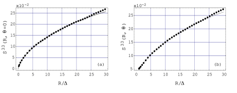
Figure 9: The structure functions computed from data set I and fit with the $j=0$ and full $j=2$ tensor contributions using the best fit values of exponents $\zeta_{2}=0.68$ and $\zeta_{2}^{(2)}=1.38$. Panel (a) shows the fit to the single-probe ($\theta=0$) structure function in the range $0.2<r/\Delta<25$ and panel (b) shows the fit to the $\theta$-dependent structure function in the range $1<r/\Delta<25$.

The corresponding values of the six fitted coefficients is given in Table 2. The range of scales that are fitted to this expression is $0.2<r/\Delta<25$ for the $\theta=0$ (single-probe) structure function and $1<r/\Delta<25$ for the $\theta\neq 0$ (two-probe) structure function. We are unable to fit Eq. (4.2.2) to scales larger than about 12 meters without losing the quality of the fit in the small scales. This limit is roughly twice the height of the probe from the ground. Based on the earlier discussion, we should be in the regime of the largest scales up to which the three-dimensional theory would hold. (Beyond this scale the boundary layer is dominated by the sloshing motions which are quasi two-dimensional in nature.) Therefore this limit to the fitting range is consistent with our expectations for the maximum scale of three-dimensional turbulence. We conclude that the structure functions exhibit scaling behavior over the whole scaling range, but this important fact is missed if one does not consider a superposition of the $j=0$ and $j=2$ contributions. We thus conclude that the estimate for the $j=2$ scaling exponent $\zeta_{2}^{(2)}\approx 1.38$. This same estimate was obtained in [4] and in the previous section using only the axisymmetric terms. The value of the coefficients $a$ and $b$ are again close in magnitude but opposite in sign—just as in [4], giving a small contribution to $S^{33}(r,\theta=0)$. The non-axisymmetric contributions vanish in the case of $\theta=0$. The contribution of these terms to the finite $\theta$ function is relatively small because the angular dependence appears as $\sin\theta$ and $\sin^{2}\theta$, both of which are small for small $\theta$ (large $r$); it was for this reason that we were able to obtain in the previous section a good fit to just the axisymmetric contribution. Lastly, we note that the total number of free parameters in this fit is 7 (6 coefficients and 1 exponent). The relative “flatness” of the $\chi^{2}$ function near its minimum (see, especially the left panel of Fig. 8) may be indicative of the large number of free parameters in the fit. However, the value of the exponent is perfectly in agreement with the analysis of numerical simulations [2] in which one can properly integrate the structure function against the basis functions, eliminating all contributions except that of the $j=2$ sector. Furthermore, fits to the data in the vicinity of $\zeta_{2}^{(2)}=1.38$ show enough divergence from experiment that we are satisfied about the genuineness of the $\chi^{2}$ result. The results of this analysis taking into account the full $j=2$ tensor were first presented in [12].

4.3 Summary

We consider the lowest order anisotropic contribution to the second order tensor functions of velocity in the atmospheric boundary layer. The $j=1$ contribution is absent in our experimental configuration because of the incompressibility constraint. The $j=2$ sector is expected to be the dominant contribution to anisotropy. First we make the a priori assumption that the cylindrical symmetry is broken in the first deviation from anisotropy. The use of the Clebsch-Gordon rules tell us the number of terms that must be included. We derive on this basis the tensor form for the $j=2$ contribution that is axisymmetric. The conditions of orthogonality with $j=0$ and incompressibility are used to constrain the unknown coefficients giving two unknown coefficients and one unknown exponent in the anisotropic sector. Using this form along with the known isotropic contribution, we can extract the anisotropic scaling exponent from the experimental data. We have also used the full form of the $j=2$ tensor including all its $2j+1$ components in order to examine if the results from the initial analysis were justified. The excellent agreement between the two strengthens our confidence in the value of the $j=2$ exponent $\zeta^{(2)}_{2}\approx 1.36$, and in our initial assumption of the breaking of axisymmetry of the flow.

5 Anisotropic contribution in the case of inhomogeneity

5.1 Extracting the j=1 component

The homogeneous structure function defined in Eq. (38) is known from properties of symmetry and parity to possess no contribution from the $j=1$ sector (see section B.2), the $j=2$ sector being its lowest order anisotropic contributor. In order to isolate the scaling behavior of the $j=1$ contribution in atmospheric shear flows we must either ($a$) explicitly construct a new tensor object which will allow for such a contribution, or ($b$) extract it from the structure function itself computed in the presence of inhomogeneity. Adopting the former approach, we construct the tensor

$$T^{\alpha\beta}({\bf r})=\langle u^{\alpha}({\bf x}+{\bf r})-u^{\alpha}({\bf x}))(u^{\beta}({\bf x}+{\bf r})+u^{\beta}({\bf x}))\rangle.$$ (43)

This object vanishes both when $\alpha=\beta$ and when ${\bf r}$ is in the direction of homogeneity, viz., the streamwise direction. From data set III we can calculate this function for non-homogeneous scale-separations (in the shear direction). In general, this will exhibit mixed parity and symmetry; the incompressibility condition does not reduce our parameter space. Therefore, to minimize the final number of fitting parameters, we examine only the antisymmetric contribution. In section B.2, we have derived the antisymmetric tensor contributions in the $j=1$ sector, and used this to fit for the unknown $j=1$ exponent. We describe the results of this effort below. This can be used to find $j=1$ exponent for the inhomogeneous structure function which is symmetric but has mixed parity. We do not present the result of that analysis here essentially because it is consistent with those from the antisymmetric case.

Returning to consideration of the antisymmetric part of the tensor object defined in Eq. (43), viz.,

$${\widetilde{T}}^{\alpha\beta}({\bf r}) = {T^{\alpha\beta}({\bf r})-T^{\beta\alpha}({\bf r})\over 2}$$ (44)

$$= \langle u^{\alpha}({\bf x})u^{\beta}({\bf x}+{\bf r})\rangle-\langle u^{\beta}({\bf x})u^{\alpha}({\bf x}+{\bf r})\rangle,$$

it is easy to see that it will only have contributions from the antisymmetric $j=1$ basis tensors. An additional useful property of this object is that, for the configuration of data set II, it does not have any contribution from the isotropic $j=0$ sector spanned by $\delta^{\alpha\beta}$ and $r^{\alpha}r^{\beta}$ since these objects are symmetric in the indices. This allows us to isolate the $j=1$ contribution and determine its scaling exponent $\zeta_{2}^{(1)}$ starting from the smallest scales available. Using data (set III) from the probes at $0.27$ m (probe 1) and at $0.11$ m (probe 2) we calculate

$${\widetilde{T}}^{31}({\bf r})=\langle u_{2}^{(3)}({\bf x})u_{1}^{(1)}({\bf x}+{\bf r})\rangle-\langle u_{1}^{(3)}({\bf x}+{\bf r})u_{2}^{(1)}({\bf x})\rangle\,$$ (45)

where again superscripts denote the velocity component and subscripts denote the probe by which this component is measured. The goal is to fit this experimental object to the tensor form derived in appendix B, Eq. (67), namely,

$${\widetilde{T}}^{31}(r,\theta,\phi=0)=-a_{3,1,0}r^{\zeta_{2}^{(1)}}\sin\theta+a_{2,1,1}r^{\zeta_{2}^{(1)}}+a_{3,1,-1}r^{\zeta_{2}^{(1)}}\cos\theta.$$ (46)

Figure 10 gives the $\chi^{2}$ minimization of the fit as a function of $\zeta_{2}^{(1)}$. We obtain the best value to be $1\pm 0.15$ for the final fit. This is shown in Fig. 11.

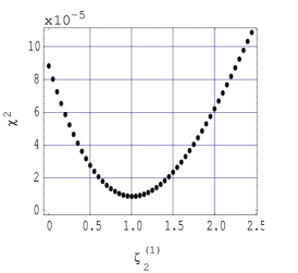
Figure 10: The $\chi^{2}$ minimization by the best-fit value of the exponent $\zeta_{2}^{(1)}$ of the $j=1$ anisotropic sector from the fit to $\theta$-dependent ${\widetilde{T}}^{31}(r,\theta)$ function in the range $1<r/\Delta<2.2$.

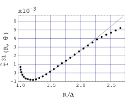
Figure 11: The fitted ${\widetilde{T}}^{31}(r,\theta)$ function. The dots indicate the data and the line is the fit.

$\zeta_{2}^{(1)}$ $a_{3,1,0}$ $a_{2,1,1}$ $a_{3,1,-1}$ $1\pm 0.15$ $0.0116\pm 0.001$ $0.0124\pm 0.001$ $-0.0062\pm 0.001$

Table 3: The values of the exponents and coefficients (in units of (m/sec)²) obtained from the fit to the function ${\widetilde{T}}^{31}(r,\theta)$.

The fit in Fig. 11 peels off at around $r/\Delta=2$. The values of the coefficients corresponding to the exponent $\zeta_{2}^{(1)}=1$ are given in Table 3. The maximum range of scales over which the fit works is of the order of the height of the probes from the ground, consistent with the considerations presented earlier. This value of the scaling exponent of the $j=1$ sector is in agreement with the theoretically expected value of unity (section 2.4). Again, we have satisfied ourselves that a different value of the exponent yields a substantially poorer fit to the data. These findings significantly strengthen the proposition [5] that the scaling exponents in the various sectors (at least up to $j=2$) are likely to be universal.

6 The higher order structure functions

6.1 Introduction

The method of SO(3) decomposition is applicable to tensor functions of any rank. However, computing the anisotropic terms in the higher order structure functions ($n>2$) becomes an increasingly difficult task. The number of contributions to a given $j$ (i.e., the $q$ index) quickly becomes too large. If we were to use the methods adopted in the case of the second order structure function, the large number of free parameters available for fitting the data guarantees over-fitting. This would not allow us to unambiguously extract the anisotropic scaling behavior. In order to circumvent this problem we recall two properties of the tensor decomposition. First, for the single-point measurements, with $\theta=0$ (no angular dependence), although the tensorial information is lost, the free coefficients collapse to a single number, see Eqs. (29) and (28). Second, the $isotropic$ part of the structure function tensor is very easily obtained, as we will show below. Examination of this part of the SO(3) expansion will show us which tensor components do not contribute to the isotropic sector. We then extract anisotropic exponents by considering only those tensor components that are explicitly zero in the isotropic sector, so that whatever is measured derives its contribution $entirely$ from the anisotropic sector. We use an interpolation formula to compensate for the large-scale encroachment of inertial-range scales. This allows us to examine the lowest order anisotropic scaling behavior. The resulting anisotropic exponents for a given tensorial order are larger than those known for the corresponding isotropic part. One conclusion that emerges is that the anisotropy effects diminish with decreasing scale, although more slowly than previously thought.

We can use the present method in principle to examine the anisotropic contribution of tensors of $any$ order without requiring the knowledge of the particular mathematical form of the anisotropic sectors of these tensors. This is a considerable advantage theoretically because the high-order tensors are non-trivial to compute; it is an advantage experimentally because, unlike in numerical simulations, one can measure only some components for simple geometric arrangements of probes. The results of this analysis were first presented in [13].

6.2 Method and results

In this part of the analysis we use data set II described in section 2. We first consider the second-order tensor $S^{\alpha\beta}({\bf r})$. Isotropy implies that this tensor can be expressed as a linear combination of two terms, $\delta^{\alpha\beta}$ and $r^{\alpha}r^{\beta}$. As is well known, both terms give non-zero contributions to longitudinal as well as transverse components, corresponding to $\alpha=\beta$. For $\alpha\neq\beta$ these two terms are identically zero if ${\bf r}$ is taken to be in the streamwise direction 3. Therefore, we compute the so-called mixed structure function

$$S^{31}(r)=\langle(u^{3}(x+r)-u^{3}(x))(u^{1}(x+r)-u^{1}(x))\rangle,$$ (47)

where, as already noted, the superscripts 1 and 3 denote the vertical and streamwise components respectively. This object is identically zero in the isotropic sector, and so, any non-zero value comes from anisotropy. In particular, any scaling behavior that it obeys should relate solely to anisotropy. By computing Eq. (47) and examining its scaling, we intend to extract the purely anisotropic scaling behavior in the $j=2$ sector, uncontaminated by any isotropic scaling, in contrast to the case of either longitudinal or transverse structure functions.

6.2.1 The second-order structure function

The previous paragraph provides the motivation for examining the measured structure functions $S^{31}(r)$. However, as we shall see shortly, apart from the expected $r^{2}$ behavior in the dissipative range and saturation at some large scale, there appears to be no distinct inertial range scaling. We suspect that this happens because there is poor scale separation, since the probes are fairly close to the ground; in fact, the large scales (which we expect to be of the order of the height of the probe from the ground and larger (see previous section)) may be encroaching significantly into the inertial range. We would be aided materially in our search for scaling if, somehow, the large-scale effects can be separated. One way of doing this is to write down an interpolation function that models the entire structure function in its three different scaling regions—a dissipative range that scales like $r^{2}$ when $r$ is of the order of the Kolmogorov scale $\eta$, a large-scale behavior that tends to saturate (indicating decorrelation) as $r$ gets to be larger than $L$, and the intermediate inertial range for $\eta<<r<<L$ which may exhibit scaling. Through the use of the interpolation formula, one can extract the scaling part in a natural way. This is described below.

A suitable form of the interpolation function is given in [6] for structure functions of arbitrary order. It has the form

$$S^{\alpha_{1}\alpha_{2}...\alpha_{n}}(r)={A_{n}\eta^{n}(r/\eta)^{n}\over(1+B_{n}(r/\eta)^{2})^{C_{n}}}(1+D_{n}(r/L))^{2C_{n}-n},$$ (48)

where $A_{n}$, $B_{n}$, $C_{n}$ and $D_{n}$ are variable parameters. This formula is an extension of that given in Ref. [28] and includes a large-scale term. Such extensions have been attempted earlier (e.g., Ref. [14]). Antonia et al. [1] have successfully tested the function (48). Dhruva [6] has shown that the present interpolation formula works extremely well for longitudinal structure functions of order 2, 4 and 6. To reinforce this point, we test its performance by comparing it to the measured transverse structure function, $\alpha=\beta=1$, $r$ in the direction 3. For each data set, the height of the probe is assumed to be the large scale $L$. The fit is shown for the transverse structure function of orders 2 and 4 at the 0.54 m probe in Fig. 12. The agreement between the formula and the data is excellent. Taken together with similar conclusions in [6] for longitudinal structure functions, we conclude that the interpolation formula describes the familiar structure functions very well. For this pragmatic reason, we shall adopt it for our purposes here, and test the robustness of the results obtained in the appendix C.

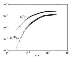
Figure 12: Log-log plots of transverse structure functions at 0.54m. $\times$ denote the second order, O the fourth order and the solid lines represent the interpolation fit.

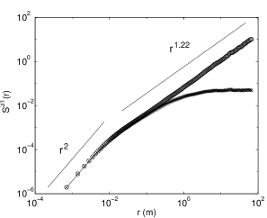
Figure 13: Log-log plot of second order mixed structure function at 0.54m. X denote data, the solid line is the interpolation fit (not visible beyond an r of $10^{-1}$m because of the closely packed symbols), and O correspond to the large-scale compensated function.

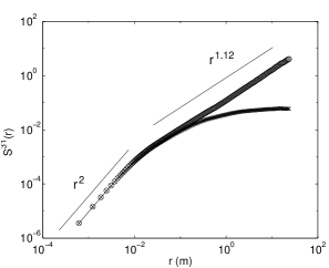
Figure 14: Log-log plot of second order mixed structure function at 0.27m. The legend is the same as for Fig. 13.

In the formula (48), the large scale behavior is given by the factor $(1+D_{2}(r/L))^{2C_{2}-2}$. If the measured structure function is divided by this factor, we should recover the contribution of the remaining parts—in particular the inertial range part, with the leading order scaling exponent given by $2-2C_{2}$. Figures 13 and 14 display a second-order anisotropic structure function for two heights above the ground. Presumably because of the finiteness of the Reynolds number and the relatively large shear effect, the scaling in the intermediate range $\eta<<r<<L$ is not apparent. However, by dividing out the large scale contribution as described above, we see two distinct regions of scaling; the dissipative range of $\sim r^{2}$ and the extended mid-range which scales with exponent between $1.22$ and $1.12$. The advantage of the scaling function is thus evident: it has allowed us to extract a scaling exponent that is most likely to be due to anisotropy. The values of the fitted parameters and the corresponding $\zeta_{2}^{(2)}$ are given in Tables 4 and 5 for the probes at 0.54 m and at 0.27 m respectively. The error on the measurement of the exponent $C_{2}$ at 0.54 m is about 0.05 while at 0.27 m it is about 0.08. This gives an error on the estimates of $\zeta_{2}^{(2)}$ of 0.07 and 0.11 respectively, and places the theoretically expected value of $\approx 4/3$ within 1.5 to 2 standard deviations of the present value. This result is consistent with general expectations [15] and the findings of the previous section.

6.2.2 Higher-order structure functions

In general, the tensor forms contributing to the $j=0$ sector for tensors of any rank $n$ are composed of linear combinations of the Kronecker-$\delta$ and the components of ${\bf r}$ along the tensor indices. The following is a list of isotropic tensor contributions for rank 3 through 6:

• $n=3$: $\delta^{\alpha\beta}r^{\gamma}$ + permutations, and $r^{\alpha}r^{\beta}r^{\gamma}$;

• $n=4$: $\delta^{\alpha\beta}\delta^{\gamma\delta}$ + permutations, $\delta^{\alpha\beta}r^{\gamma}r^{\delta}$ + permutations, and
  $r^{\alpha}r^{\beta}r^{\gamma}r^{\delta}$;

• $n=5$: $\delta^{\alpha\beta}\delta^{\gamma\delta}r^{\mu}$ + permutations, $\delta^{\alpha\beta}r^{\gamma}r^{\delta}r^{\mu}$ + permutations, and $r^{\alpha}r^{\beta}r^{\gamma}r^{\delta}r^{\mu}$;

• $n=6$: $\delta^{\alpha\beta}\delta^{\gamma\delta}\delta^{\mu\nu}$ + permutations, $\delta^{\alpha\beta}\delta^{\gamma\delta}r^{\mu}r^{\nu}$ + permutations,
  $\delta^{\alpha\beta}r^{\gamma}r^{\delta}r^{\mu}r^{\nu}$ + permutations, and $r^{\alpha}r^{\beta}r^{\gamma}r^{\delta}r^{\mu}r^{\nu}$.

Based on the above considerations, it can be expected that the structure function components that are zero in the $j=0$ sector are:

• $n=3$: $S^{111}$ (transverse), $S^{331}$;

• $n=4$: $S^{3331},S^{3111}$;

• $n=5$: $S^{11111}$ (transverse), $S^{33111},S^{33331}$;

• $n=6$: $S^{333111},S^{311111},S^{333331}$.

Note that the odd-order transverse structure function is always zero in the isotropic sector. The functions we shall now consider are given in the second column of Tables 4 and 5.

Order $n$ Tensor $A_{n}$ $B_{n}$ $C_{n}$ $D_{n}$ $\zeta_{n}^{(2)}=n-2C_{n}$ $\zeta_{n}$ 2 $S^{31}$ 3.9 0.014 0.39 0.67 1.22 0.7 3 $S^{111}$ 2400 0.010 0.93 2.28 1.14 1 4 $S^{3331}$ 5200 0.014 1.21 0.27 1.58 1.26 5 $S^{11111}$ $1.22\times 10^{7}$ 0.029 1.59 3.09 1.82 1.56 6 $S^{333111}$ $3.75\times 10^{7}$ 0.041 1.93 0.50 2.14 1.71

Table 4: Structure function calculated and the anisotropic scaling exponents for the data at 0.54m.

Order $n$ Tensor $A_{n}$ $B_{n}$ $C_{n}$ $D_{n}$ $\zeta_{n}^{(2)}=n-2C_{n}$ $\zeta_{n}$ 2 $S^{31}$ 9.4 0.005 0.44 0.52 1.12 0.7 3 $S^{111}$ 6940 0.015 0.89 2.78 1.21 1 4 $S^{3331}$ $2.1\times 10^{4}$ 0.014 1.23 0.23 1.54 1.26 5 $S^{11111}$ $5.9\times 10^{7}$ 0.028 1.58 3.52 1.84 1.56 6 $S^{333111}$ $2.7\times 10^{8}$ 0.038 2.00 0.34 2.00 1.71

Table 5: Structure function calculated and the anisotropic scaling exponents for the data at 0.27m.

For the case of the third and fifth order transverse structure functions we use the moments of the absolute value of the velocity differences in order to obtain better convergence. In using the interpolation function we assume that the inertial range scaling of these anisotropic components is given by a single exponent $\zeta_{n}^{(j)}$ where the superscript denotes an isotropic exponent without reference to the precise $j$ sector. The compensated functions (with large-scale effects removed) are shown in Figs. 15–22. The errors on the value of $\zeta_{n}^{(2)}$ obtained are about $7\%$ at 0.54 m and about $9\%$ at 0.27 m. For comparison, the last column in Tables 4 and 5 gives the empirical values of the isotropic scaling exponent of the same order as given in [6]. The entries in this column are measurably smaller than the corresponding non-isotropic exponents. This suggests that the isotropic component alone survives at very small scales.

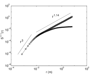
Figure 15: Log-log plot of third-order transverse structure function at 0.54m. The legend is the same as for Fig. 13.

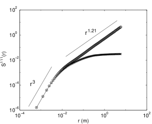
Figure 16: Log-log plot of third-order transverse structure function at 0.27m. The legend is the same as for Fig. 13.

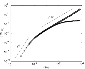
Figure 17: Log-log plot of fourth-order mixed structure function at 0.54m. The legend is the same as for Fig. 13.

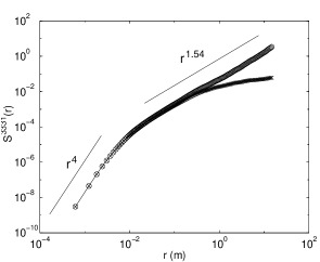
Figure 18: Log-log plot of fourth-order mixed structure function at 0.27m. The legend is the same as for Fig. 13.

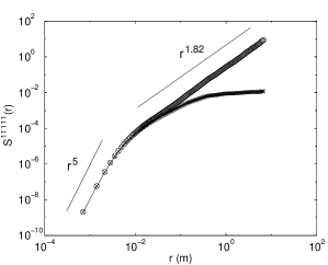
Figure 19: Log-log plot of fifth-order transverse structure function at 0.54m. The legend is the same as for Fig. 13.

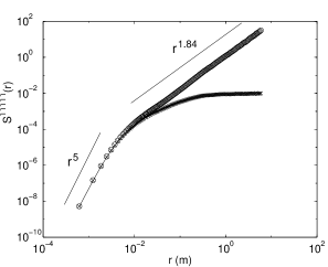
Figure 20: Log-log plot of fifth-order transverse structure function at 0.27m. The legend is the same as for Fig. 13.

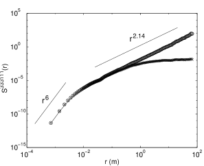
Figure 21: Log-log plot of sixth-order mixed structure function at 0.54m. The legend is the same as for Fig. 13.

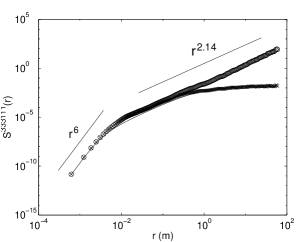
Figure 22: Log-log plot of sixth-order mixed structure function at 0.27m. The legend is the same as for Fig. 13.

6.3 Summary

We have presented a new method of extracting anisotropic exponents that avoids mixing with contributions from the isotropic sector. We do this by explicitly constructing those tensors that are zero in the isotropic sector. An operational step in the extraction of the scaling exponents is the use of an interpolation formula in the spirit of a “scaling function”. This method has allowed us to examine anisotropic effects in structure function tensors of order greater than 2. The resulting anisotropic exponents are consistently larger than those known for isotropic parts at all orders. This strongly suggests that anisotropy effects decrease with decreasing scale. However, the rate of decrease is much slower than expected from dimensional arguments (which yield 4/3, 5/3, 2, 7/3 and 8/3 for orders 2 through 6, to be compared with the values obtained at $0.54$ m of 1.22, 1.14, 1.58, 1.82, 2.14).

Our conclusions are based on the use of the interpolation formula, given by Eq. (48). While this formula is not based on a solid theoretical framework, we have shown that it works very well in describing the measured structure functions. We have also performed tests of its robustness by fitting it to smaller sections of the data in order to detect changes in the exponent. A discussion of these checks and their results is presented in appendix C. To the lowest order, the results are independent of the $r$-segment to which the formula is fitted (except, of course, when the fit is entirely for the dissipation range or in the large-scale range). Any other formula that works equally well will yield similar results. Even so, the formula is empirical, which is why we have not paid much attention to the fact that the scaling exponents obtained for the two probe positions are slightly different, and that the second-order exponent for 0.54 m is slightly larger than that obtained for the third-order. On the whole, the trend is that the anisotropic exponents become larger for larger orders of the structure function.

An interesting conclusion of the present work is that the effects of anisotropy vanish with decreasing scale more slowly than expected. The expectation in the light of the SO(3) formalism is that a hierarchy of increasingly larger exponents, corresponding to increasingly higher-order anisotropic sectors [17], would exist. This expectation appears to be true in the case of the passively advected vector field [3] where a discrete spectrum of anisotropic scaling exponents is obtained theoretically for all anisotropic sectors. In the present experiments, the fact that anisotropic effects can be fitted reasonably well by power laws suggests that the high-order effects may be small. It is perhaps true, however, that the power-laws described here may contain high-order corrections, and that the exponents deduced for the behavior of anisotropy may indeed undergo some revision when contributions from other sectors of the SO(3) decomposition are also considered. In spite of this possibility, we wish to emphasize that the anisotropy effects for each order of the structure function appear to be well described by something close to a power law with a single exponent. The magnitudes of the anisotropic exponents in each order indicate that the roll-off from isotropy happens less sharply than previously thought, but the roll-off occurs nevertheless. The higher-order objects considered here have not been studied extensively in the light of anisotropy.

7 Conclusions

We have used the SO(3) decomposition of tensorial objects such as structure functions measured in fluid turbulence experiments. This enables us to separate, for any given order structure function, the isotropic part from the anisotropic part. We have used experimental data at very high Reynolds numbers (Taylor microscale Reynolds numbers of up to 20,000) to carry through this decomposition.

We considered the lowest order anisotropic contribution to the second order tensor functions of velocity in the atmospheric boundary layer. For second order structure functions, we have extracted the anisotropic scaling exponent from the experimental data. We also used the full form of the $j=2$ tensor, as well as the axisymmetric version of it. In both instances, we have shown that the $j=2$ exponent $\zeta^{(2)}_{2}\approx 1.36$. This compares favorably with the estimate based on purely dimensional grounds. It should be noted that the dimensional estimates do not take into account possible anomalous scaling. We expect that turbulence flows will exhibit anomalous scaling in the isotropic sector, and in every anisotropic sector in the SO(3) hierarchy. By suitably arranging the measurement configuration, we have also extracted the $j=1$ contribution, and find the appropriate scaling exponent to be close to the dimensional estimate of unity.

For high orders, we have presented a new method for the extraction of anisotropic exponents that avoids mixing with contributions from the isotropic sector. We do this by explicitly constructing those tensors that are zero in the isotropic sector. The resulting anisotropic exponents are consistently larger than those known for isotropic parts at all orders. This strongly suggests that anisotropy effects decrease with decreasing scale. However, the rate of decrease is slower than expected from dimensional arguments (which yield 4/3, 5/3, 2, 7/3 and 8/3 for orders 2 through 6, to be compared with the values obtained at $0.54$ m of 1.22, 1.14, 1.58, 1.82, 2.14).

Armed with these details, it is now possible to say something of value about local isotropy. These statements are interspersed through out the text, but the most important conclusion is that the effects of anisotropy within a structure function of a given order do vanish with decreasing scale, though more slowly than expected. This provides a rich perspective on the notion of local isotropy and removes a hurdle towards the search for a universal theory of small-scale turbulence.

Appendix A Full form for the $j=2$ contribution for the homogeneous case

Each index $j$ in the SO(3) decomposition of an $n$-rank tensor labels a $2j+1$ dimensional SO(3) representation. Each dimension is labeled by $m=-j,-j+1,\dots j$. The $j=0$ sector is the isotropic contribution while higher order $j$’s should describe any anisotropy. The $j=0$ terms are well known to be

$$S_{j=0}^{\alpha\beta}({\bf r})=c_{0}r^{\zeta_{2}}\left[(2+\zeta_{2})\delta^{\alpha\beta}-\zeta_{2}{r^{\alpha}r^{\beta}\over r^{2}}\right]\,$$ (49)

where $\zeta_{2}\approx 0.69$ is the known universal scaling exponent for the isotropic contribution, and $c_{0}$ is an unknown coefficient that depends on the boundary conditions of the flow. For the $j=2$ sector, which is the lowest contribution to anisotropy to the homogeneous structure function, the $m=0$ (axisymmetric) terms were derived from constraints of symmetry, even parity (because of homogeneity) and incompressibility on the second order structure function to be [4]

$$S^{\alpha\beta}_{j=2,m=0}({\bf r})=ar^{\zeta_{2}^{(2)}}\Big{[}(\zeta_{2}^{(2)}-2)\delta^{\alpha\beta}-\zeta_{2}^{(2)}(\zeta_{2}^{(2)}+6)$$

$$\times \delta^{\alpha\beta}{({\bf n}\cdot{\bf r})^{2}\over r^{2}}+2\zeta_{2}^{(2)}(\zeta_{2}^{(2)}-2){r^{\alpha}r^{\beta}({\bf n}\cdot{\bf r})^{2}\over r^{4}}$$

$$+ ([\zeta_{2}^{(2)}]^{2}+3\zeta_{2}^{(2)}+6)n^{\alpha}n^{\beta}$$

$$- {\zeta_{2}^{(2)}(\zeta_{2}^{(2)}-2)\over r^{2}}(r^{\alpha}n^{\beta}+r^{\beta}n^{\alpha})({\bf n}\cdot{\bf r})\Big{]}$$

$$+ br^{\zeta_{2}^{(2)}}\Big{[}-(\zeta_{2}^{(2)}+3)(\zeta_{2}^{(2)}+2)\delta^{\alpha\beta}({\bf n}\cdot{\bf r})^{2}+{r^{\alpha}r^{\beta}\over r^{2}}$$

$$+ (\zeta_{2}^{(2)}+3)(\zeta_{2}^{(2)}+2)n^{\alpha}n^{\beta}+(2\zeta_{2}^{(2)}+1)(\zeta_{2}^{(2)}-2)$$

$$\times {{r^{\alpha}}{r^{\beta}}{({\bf n}\cdot{\bf r})^{2}}\over r^{4}}-([\zeta_{2}^{(2)}]^{2}-4)(r^{\alpha}n^{\beta}+r^{\beta}n^{\alpha})({\bf n}\cdot{\bf r})\Big{]}.$$

Here $\zeta_{2}^{(2)}$ is the universal scaling exponent for the $j=2$ anisotropic sector and $a$ and $b$ are independent unknown coefficients to be determined by the boundary conditions. We would now like to derive the remaining $m=\pm 1$, and $m=\pm 2$ components

$$S_{j=2,m}^{\alpha\beta}=\sum_{q}{a_{q,2,m}r^{\zeta_{2}^{(2)}}B_{q,2,m}^{\alpha\beta}(\bf{\hat{r}})},$$ (51)

where $\zeta_{2}^{2}$ is the scaling exponent of the $j=2$ SO(3) representation of the $n=2$ rank correlation function. The $B_{q,j,m}^{\alpha\beta}(\bf{\hat{r}})$ are the basis functions in the SO(3) representation of the structure function. The $q$ label denotes the different possible ways of arriving at the the same $j$ and runs over all such terms with the same parity and symmetry (a consequence of homogeneity and hence the constraint of incompressibility); see Ref. [5]. In our case, even parity and symmetric in the two indices. In all that follows, we work closely with the procedure outlined in [5]. Following the convention in [5] the $q$’s to sum over are $q=\{1,7,9,5\}$. The incompressibility condition $\partial_{\alpha}u^{\alpha}=0$ coupled with homogeneity can be used to give relations between the $a_{q,j,m}$ for a given $(j,m)$. That is, for $j=2$, $m=-2\dots 2$, we have

$$(\zeta_{2}^{(2)}-2)a_{1,2,m}+2(\zeta_{2}^{(2)}-2)a_{7,2,m}+(\zeta_{2}^{(2)}+2)a_{9,2,m} = 0$$

$$a_{1,2,m}+(\zeta_{2}^{(2)}+3)a_{7,2,m}+\zeta_{2}^{(2)}a_{5,2,m} = 0.$$ (52)

We solve equations (3) in order to obtain $a_{5,2,m}$ and $a_{7,2,m}$ in terms of linear combinations of $a_{1,2,m}$ and $a_{9,2,m}$:

$$a_{5,2,m} = {a_{1,2,m}([\zeta_{2}^{(2)}]^{2}-\zeta_{2}^{(2)}-2)+a_{9,2,m}([\zeta_{2}^{(2)}]^{2}+5\zeta_{2}^{(2)}+6)\over 2\zeta_{2}^{(2)}(\zeta_{2}^{(2)}-2)}$$

$$a_{7,2,m} = {a_{1,2,m}(2-\zeta_{2}^{(2)})-a_{9,2,m}(2+\zeta_{2}^{(2)})\over 2(\zeta_{2}^{(2)}-2)}.$$ (53)

Using the above constraints on the coefficients, we are now left with a linear combination of just two linearly independent tensor forms for each m:

$$S^{\alpha\beta}_{j=2,m} = a_{9,2,m}r^{\zeta_{2}^{(2)}}[-\zeta_{2}^{(2)}(2+\zeta_{2}^{(2)})B_{7,2,m}^{\alpha\beta}({\bf{\hat{r}}})$$

$$\mbox{~{}}\hskip 42.67912pt+2\zeta_{2}^{(2)}(\zeta_{2}^{(2)}-2)B_{9,2,m}^{\alpha\beta}({\bf{\hat{r}}})$$

$$\mbox{~{}}\hskip 42.67912pt+([\zeta_{2}^{(2)}]^{2}+5\zeta_{2}^{(2)}+6)B_{5,2,m}^{\alpha\beta}({\bf{\hat{r}}})]$$

$$+ a_{1,2,m}r^{\zeta_{2}^{(2)}}[2\zeta_{2}^{(2)}(\zeta_{2}^{(2)}-2)B_{1,2,m}^{\alpha\beta}({\bf{\hat{r}}})$$

$$\mbox{~{}}\hskip 42.67912pt-\zeta_{2}^{(2)}(\zeta_{2}^{(2)}-2)B_{7,2,m}^{\alpha\beta}({\bf{\hat{r}}})$$

$$\mbox{~{}}\hskip 42.67912pt+([\zeta_{2}^{(2)}]^{2}-\zeta_{2}^{(2)}-2)B_{5,2,m}^{\alpha\beta}({\bf{\hat{r}}})].$$

The task remains to find the explicit form of the basis tensor functions $B_{q,2,m}^{\alpha\beta}({\bf{\hat{r}}})$, $q\in\{1,7,9,5\}$, $m\in\{\pm 1,\pm 2\}$
$\bullet$ $B_{1,2,m}^{\alpha\beta}({\bf{\hat{r}}})\equiv r^{-2}\delta^{\alpha\beta}r^{j}Y_{2m}({\bf{\hat{r}}})$
$\bullet$ $B_{7,2,m}^{\alpha\beta}({\bf{\hat{r}}})\equiv r^{-2}[r^{\alpha}\partial^{\beta}+r^{\beta}\partial^{\alpha}]r^{2}Y_{2m}({\bf{\hat{r}}})$
$\bullet$ $B_{9,2,m}^{\alpha\beta}({\bf{\hat{r}}})\equiv r^{-4}r^{\alpha}r^{\beta}r^{2}Y_{2m}({\bf{\hat{r}}})$
$\bullet$ $B_{5,2,m}^{\alpha\beta}({\bf{\hat{r}}})\equiv\partial^{\alpha}\partial^{\beta}r^{2}Y_{jm}({\bf{\hat{r}}}).$

We obtain the $m=\{\pm 1,\pm 2\}$ basis functions in the following derivation. We first note that it is more convenient to form a real basis from the $r^{2}Y_{2m}({\bf{\hat{r}}})$ since we ultimately wish to fit to real quantities and extract real best-fit parameters. We therefore form the $r^{2}{\widetilde{Y}}_{2k}({\bf{\hat{r}}})$ ($k=-1,0,1$) as follows:

$$r^{2}{\widetilde{Y}}_{2\;0}(\hat{\bf r}) = r^{2}Y_{2\;0}(\hat{\bf r})=r^{2}\cos^{2}\theta=r{{}_{3}}^{2}$$

$$r^{2}{\widetilde{Y}}_{2\;-1}(\hat{\bf r}) = r^{2}{Y_{2\;-1}(\hat{\bf r})-Y_{2\;+1}(\hat{\bf r})\over 2}$$

$$= {r^{2}\over 2}\Big{[}(\cos\phi-i\sin\phi)\cos\theta\sin\theta$$

$$\hskip 19.91684pt+(\cos\phi+i\sin\phi)\cos\theta\sin\theta\Big{]}$$

$$= r^{2}\cos\theta\sin\theta\cos\phi=r_{3}r_{1}$$

$$r^{2}{\widetilde{Y}}_{2\;+1}(\hat{\bf r}) = r^{2}{Y_{2\;-1}(\hat{\bf r})+Y_{2\;+1}(\hat{\bf r})\over-2i}$$

$$= {r^{2}\over-2i}\Big{[}(\cos\phi-i\sin\phi)\cos\theta\sin\theta$$

$$\hskip 19.91684pt-(\cos\phi+i\sin\phi)\cos\theta\sin\theta\Big{]}$$

$$= r^{2}\cos\theta\sin\theta\sin\phi=r_{3}r_{2}$$

$$r^{2}{\widetilde{Y}}_{2\;-2}(\hat{\bf r}) = r^{2}{Y_{2\;2}(\hat{\bf r})-Y_{2\;-2}(\hat{\bf r})\over 2i}$$

$$= {r^{2}\over 2i}\Big{[}(\cos 2\phi+i\sin 2\phi)\sin^{2}\theta-(\cos 2\phi-i\sin 2\phi)\sin^{2}\theta\Big{]}$$

$$= r^{2}\sin 2\phi\sin^{2}\theta=2r_{1}r_{2}$$

$$r^{2}{\widetilde{Y}}_{2\;+2}(\hat{\bf r}) = r^{2}{Y_{2\;2}(\hat{\bf r})+Y_{2\;-2}(\hat{\bf r})\over 2}$$ (55)

$$= {r^{2}\over 2}\Big{[}(\cos 2\phi+i\sin 2\phi)\sin^{2}\theta+(\cos 2\phi-i\sin 2\phi)\sin^{2}\theta\Big{]}$$

$$= r^{2}\cos 2\phi\sin^{2}\theta=r_{1}^{2}-r_{2}^{2}.$$

This new basis of $r^{2}{\tilde{Y}}_{2k}{(\bf r)}$ is equivalent to the $r^{2}Y_{jm}{(\bf r)}$ themselves as they form a complete, orthogonal set (in the new k’s). We omit the normalization constants for the spherical harmonics for notational convenience. The subscripts on $r$ denote its components along the 1 ($m$), 2 ($p$) and 3 ($n$) directions; ${\bf m}$ denotes the shear direction, ${\bf p}$ the horizontal direction parallel to the boundary and orthogonal to the mean wind direction and ${\bf n}$ the direction of the mean wind. This notation simplifies the derivatives when we form the different basis tensors; the only thing to remember is that

$$\partial^{\alpha}r_{1}=\partial^{\alpha}(\bf{r\cdot m})=m^{\alpha}$$

$$\partial^{\alpha}r_{2}=\partial^{\alpha}(\bf{r\cdot p})=p^{\alpha}$$

$$\partial^{\alpha}r_{3}=\partial^{\alpha}(\bf{r\cdot n})=n^{\alpha}.$$ (56)

We use the above identities to proceed to derive the basis tensor functions

$$B_{1,2,-1}^{\alpha\beta}({\bf{\hat{r}}}) = r^{-2}\delta^{\alpha\beta}({\bf r\cdot n})({\bf r\cdot m})$$

$$B_{7,2,-1}^{\alpha\beta}({\bf{\hat{r}}}) = r^{-2}[(r^{\alpha}m^{\beta}+r^{\beta}m^{\alpha})({\bf r\cdot n})+(r^{\alpha}n^{\beta}+r^{\beta}n^{\alpha})({\bf r\cdot m})]$$

$$B_{9,2,-1}^{\alpha\beta}({\bf{\hat{r}}}) = r^{-2}r^{\alpha}r^{\beta}({\bf r\cdot n})({\bf r\cdot m})$$

$$B_{5,2,-1}^{\alpha\beta}({\bf{\hat{r}}}) = n^{\alpha}m^{\beta}+n^{\beta}m^{\alpha}$$

$$B_{1,2,1}^{\alpha\beta}({\bf{\hat{r}}}) = r^{-2}\delta^{\alpha\beta}({\bf r\cdot n})({\bf r\cdot p})$$

$$B_{7,2,1}^{\alpha\beta}({\bf{\hat{r}}}) = r^{-2}[(r^{\alpha}p^{\beta}+r^{\beta}p^{\alpha})({\bf r\cdot n})+(r^{\alpha}n^{\beta}+r^{\beta}n^{\alpha})({\bf r\cdot p})]$$

$$B_{9,2,1}^{\alpha\beta}({\bf{\hat{r}}}) = r^{-2}r^{\alpha}r^{\beta}({\bf r\cdot n})({\bf r\cdot p})$$

$$B_{5,2,1}^{\alpha\beta}({\bf{\hat{r}}}) = n^{\alpha}p^{\beta}+n^{\beta}p^{\alpha}$$

$$B_{1,2,-2}^{\alpha\beta}({\bf{\hat{r}}}) = 2r^{-2}\delta^{\alpha\beta}({\bf r\cdot m})({\bf r\cdot p})$$

$$B_{7,2,-2}^{\alpha\beta}({\bf{\hat{r}}}) = 2r^{-2}[(r^{\alpha}p^{\beta}+r^{\beta}p^{\alpha})({\bf r\cdot m})+(r^{\alpha}m^{\beta}+r^{\beta}m^{\alpha})({\bf r\cdot p})]$$

$$B_{9,2,-2}^{\alpha\beta}({\bf{\hat{r}}}) = 2r^{-2}r^{\alpha}r^{\beta}({\bf r\cdot m})({\bf r\cdot p})$$

$$B_{5,2,-2}^{\alpha\beta}({\bf{\hat{r}}}) = 2(m^{\alpha}p^{\beta}+m^{\beta}p^{\alpha})$$

$$B_{1,2,2}^{\alpha\beta}({\bf{\hat{r}}}) = r^{-2}\delta^{\alpha\beta}[({\bf r\cdot m})^{2}-({\bf r\cdot p})^{2}]$$

$$B_{7,2,2}^{\alpha\beta}({\bf{\hat{r}}}) = 2r^{-2}[(r^{\alpha}m^{\beta}+r^{\beta}m^{\alpha})({\bf r\cdot m})-(r^{\alpha}p^{\beta}+r^{\beta}p^{\alpha})({\bf r\cdot p})]$$

$$B_{9,2,2}^{\alpha\beta}({\bf{\hat{r}}}) = r^{-2}r^{\alpha}r^{\beta}[({\bf r\cdot m})^{2}-({\bf r\cdot p})^{2}]$$

$$B_{5,2,2}^{\alpha\beta}({\bf{\hat{r}}}) = 2(m^{\alpha}m^{\beta}-p^{\alpha}p^{\beta}).$$ (57)

Substituting these tensors forms into Eq. A we obtain the full tensor forms for the $j=2$ non-axisymmetric terms, with two independent coefficients for each k:

$$S^{\alpha\beta}_{j=2,k=-1}({\bf r}) = a_{9,2,-1}r^{\zeta_{2}^{(2)}}{\Big{[}}([\zeta_{2}^{(2)}]^{2}+5\zeta_{2}^{(2)}+6)(n^{\alpha}m^{\beta}+n^{\beta}m^{\alpha})$$

$$+ 2\zeta_{2}^{(2)}(\zeta_{2}^{(2)}-2)r^{-4}r^{\alpha}r^{\beta}({\bf r\cdot n})({\bf r\cdot m})$$

$$- \zeta_{2}^{(2)}(2+\zeta_{2}^{(2)})r^{-2}[(r^{\alpha}m^{\beta}+r^{\beta}m^{\alpha})({\bf r\cdot n})$$

$$~{}\hskip 71.13188pt+(r^{\alpha}n^{\beta}+r^{\beta}n^{\alpha})({\bf r\cdot m})]{\Big{]}}$$

$$+ a_{1,2,-1}r^{\zeta_{2}^{(2)}}{\Big{[}}([\zeta_{2}^{(2)}]^{2}-\zeta_{2}^{(2)}-2)(n^{\alpha}m^{\beta}+n^{\beta}m^{\alpha})$$

$$+ 2\zeta_{2}^{(2)}(\zeta_{2}^{(2)}-2)r^{-2}\delta^{\alpha\beta}({\bf r\cdot n})({\bf r\cdot m})$$

$$- \zeta_{2}^{(2)}(\zeta_{2}^{(2)}-2)r^{-2}[(r^{\alpha}m^{\beta}+r^{\beta}m^{\alpha})({\bf r\cdot n})$$

$$~{}\hskip 71.13188pt+(r^{\alpha}n^{\beta}+r^{\beta}n^{\alpha})({\bf r\cdot m})]{\Big{]}}$$

$$S^{\alpha\beta}_{j=2,k=1}({\bf r}) = a_{9,2,1}r^{\zeta_{2}^{(2)}}{\Big{[}}([\zeta_{2}^{(2)}]^{2}+5\zeta_{2}^{(2)}+6)(n^{\alpha}p^{\beta}+n^{\beta}p^{\alpha})$$

$$+ 2\zeta_{2}^{(2)}(\zeta_{2}^{(2)}-2)r^{-4}r^{\alpha}r^{\beta}({\bf r\cdot n})({\bf r\cdot p})$$

$$- \zeta_{2}^{(2)}(2+\zeta_{2}^{(2)})r^{-2}[(r^{\alpha}p^{\beta}+r^{\beta}p^{\alpha})({\bf r\cdot n})$$

$$~{}\hskip 71.13188pt+(r^{\alpha}n^{\beta}+r^{\beta}n^{\alpha})({\bf r\cdot p})]{\Big{]}}$$

$$+ a_{1,2,1}r^{\zeta_{2}^{(2)}}{\Big{[}}([\zeta_{2}^{(2)}]^{2}-\zeta_{2}^{(2)}-2)(n^{\alpha}p^{\beta}+n^{\beta}p^{\alpha})$$

$$+ 2\zeta_{2}^{(2)}(\zeta_{2}^{(2)}-2)r^{-2}\delta^{\alpha\beta}({\bf r\cdot n})({\bf r\cdot p})$$

$$- \zeta_{2}^{(2)}(\zeta_{2}^{(2)}-2)r^{-2}[(r^{\alpha}p^{\beta}+r^{\beta}p^{\alpha})({\bf r\cdot n})$$

$$~{}\hskip 71.13188pt+(r^{\alpha}n^{\beta}+r^{\beta}n^{\alpha})({\bf r\cdot p})]{\Big{]}}$$

$$S^{\alpha\beta}_{j=2,k=-2}({\bf r}) = a_{9,2,-2}r^{\zeta_{2}^{(2)}}{\Big{[}}([\zeta_{2}^{(2)}]^{2}+5\zeta_{2}^{(2)}+6)(m^{\alpha}p^{\beta}+m^{\beta}p^{\alpha})$$

$$+ 2\zeta_{2}^{(2)}(\zeta_{2}^{(2)}-2)r^{-4}r^{\alpha}r^{\beta}({\bf r\cdot p})({\bf r\cdot m})$$

$$- 2\zeta_{2}^{(2)}(2+\zeta_{2}^{(2)})r^{-2}[(r^{\alpha}p^{\beta}+r^{\beta}p^{\alpha})({\bf r\cdot m})$$

$$~{}\hskip 71.13188pt+(r^{\alpha}m^{\beta}+r^{\beta}m^{\alpha})({\bf r\cdot p})]{\Big{]}}$$

$$+ a_{1,2,-2}r^{\zeta_{2}^{(2)}}{\Big{[}}2([\zeta_{2}^{(2)}]^{2}-\zeta_{2}^{(2)}-2)(m^{\alpha}p^{\beta}+m^{\beta}p^{\alpha})$$

$$+ 2\zeta_{2}^{(2)}(\zeta_{2}^{(2)}-2)r^{-2}\delta^{\alpha\beta}({\bf r\cdot m})({\bf r\cdot p})$$

$$- 2\zeta_{2}^{(2)}(\zeta_{2}^{(2)}-2)r^{-2}[(r^{\alpha}p^{\beta}+r^{\beta}p^{\alpha})({\bf r\cdot m})$$

$$~{}\hskip 71.13188pt+(r^{\alpha}m^{\beta}+r^{\beta}m^{\alpha})({\bf r\cdot p})]{\Big{]}}$$

$$S^{\alpha\beta}_{j=2,k=2}({\bf r}) = a_{9,2,2}r^{\zeta_{2}^{(2)}}{\Big{[}}2([\zeta_{2}^{(2)}]^{2}+5\zeta_{2}^{(2)}+6)(m^{\alpha}m^{\beta}-p^{\beta}p^{\alpha})$$ (58)

$$+ 2\zeta_{2}^{(2)}(\zeta_{2}^{(2)}-2)r^{-4}r^{\alpha}r^{\beta}[({\bf r\cdot m})^{2}-({\bf r\cdot p})^{2}]$$

$$- 2\zeta_{2}^{(2)}(2+\zeta_{2}^{(2)})r^{-2}[(r^{\alpha}m^{\beta}+r^{\beta}m^{\alpha})({\bf r\cdot m})$$

$$~{}\hskip 71.13188pt-(r^{\alpha}p^{\beta}+r^{\beta}p^{\alpha})({\bf r\cdot p})]{\Big{]}}$$

$$+ a_{1,2,2}r^{\zeta_{2}^{(2)}}{\Big{[}}2([\zeta_{2}^{(2)}]^{2}-\zeta_{2}^{(2)}-2)(m^{\alpha}m^{\beta}-p^{\beta}p^{\alpha})$$

$$+ 2\zeta_{2}^{(2)}(\zeta_{2}^{(2)}-2)r^{-2}\delta^{\alpha\beta}[({\bf r\cdot m})^{2}-({\bf r\cdot p})^{2}]$$

$$- 2\zeta_{2}^{(2)}(\zeta_{2}^{(2)}-2)r^{-2}[(r^{\alpha}m^{\beta}+r^{\beta}m^{\alpha})({\bf r\cdot m})$$

$$~{}\hskip 71.13188pt-(r^{\alpha}p^{\beta}+r^{\beta}p^{\alpha})({\bf r\cdot p})]{\Big{]}}.$$

Now we wish to use this form to fit for the scaling exponent $\zeta_{2}^{(2)}$ in the structure function $S^{33}({\bf r})$ from data set I where $\alpha=\beta=3$ and the azimuthal angle of ${\bf r}$ in the geometry is $\phi=\pi/2$.:

$$S^{33}_{j=2,k=-1}(r,\theta,\phi=\pi/2) = 0$$

$$S^{33}_{j=2,k=1}(r,\theta,\phi=\pi/2) = a_{9,2,1}r^{\zeta_{2}^{(2)}}[-2\zeta_{2}^{(2)}(\zeta_{2}^{(2)}+2)\sin\theta\cos\theta$$

$$+ 2\zeta_{2}^{(2)}(\zeta_{2}^{(2)}-2)\cos^{3}\theta\sin\theta]$$

$$S^{33}_{j=2,k=-2}(r,\theta,\phi=\pi/2) = 0$$

$$S^{33}_{j=2,k=2}(r,\theta,\phi=\pi/2) = a_{9,2,2}r^{\zeta_{2}^{(2)}}[-2\zeta_{2}^{(2)}(\zeta_{2}^{(2)}-2)\cos^{2}\theta\sin^{2}\theta]$$ (59)

$$+ a_{1,2,2}r^{\zeta_{2}^{(2)}}[-2\zeta_{2}^{(2)}(\zeta_{2}^{(2)}-2)\sin^{2}\theta].$$

Table 6: The number of free coefficients in the $j=2$ sector for homogeneous turbulence and for different geometries

We see that choosing a particular geometry eliminates certain tensor contributions. In the case of set I we are left with 3 independent coefficients for $m\neq 0$, the 2 coefficients from the $m=0$ contribution (Eq. A), and the single coefficient from the isotropic sector 49, giving a total of 6 fit parameters. The general forms in A can be used along with the $k=0$ (axisymmetric) contribution 49 to fit to any second order tensor object. For convenience, Table 6 shows the number of independent coefficients that a few different experimental geometries we have will allow in the $j=2$ sector. It must be kept in mind that these forms are to be used only when homogeneity is known to exist. If there is inhomogeneity, the incompressibility condition cannot be used to provide constraints in the various parity and symmetry sectors, and we must in general mix different parity objects using only the geometry of the experiment itself to eliminate any terms.

Appendix B The j=1 component in the inhomogeneous case

B.1 Antisymmetric contribution

We consider the tensor

$$T^{\alpha\beta}({\bf r})=<u^{\alpha}({\bf x}+{\bf r})-u^{\alpha}({\bf x}))(u^{\beta}({\bf x}+{\bf r})+u^{\beta}({\bf x}))>.$$ (60)

This object is trivially zero for $\alpha=\beta$. In our experimental setup, we measure at points separated in the shear direction and therefore have inhomogeneity which makes the object of mixed parity and symmetry. We cannot apply the incompressibility condition in same parity/symmetry sectors as before to provide constraints. We must in general use all 7 irreducible tensor forms. This would mean fitting for $7\times 3=21$ independent coefficients plus 1 exponent $\zeta_{2}^{(1)}$ in the anisotropic sector, together with 2 coefficients in the isotropic sector. In order to pare down the number of parameters we are fitting for, we look at the antisymmetric part of $T^{\alpha\beta}({\bf r})$,

$${\widetilde{T}}^{\alpha\beta}({\bf r})={T^{\alpha\beta}({\bf r})-T^{\beta\alpha}({\bf r})\over 2}=\langle u^{\alpha}({\bf x})u^{\beta}({\bf x}+{\bf r})\rangle-\langle u^{\beta}({\bf x})u^{\alpha}({\bf x}+{\bf r})\rangle,$$ (61)

which will only have contributions from the antisymmetric $j=1$ basis tensors. These are:
$\bullet$ Antisymmetric, odd parity

$$B_{3,1,m}^{\alpha\beta}=r^{-1}[r^{\alpha}\partial^{\beta}-r^{\beta}\partial^{\alpha}]rY_{1,m}(\bf{\hat{r}})$$ (62)

$\bullet$ Antisymmetric, even parity

$$B_{4,1,m}^{\alpha\beta} = r^{-2}\epsilon^{\alpha\beta\mu}r_{\mu}rY_{1,m}(\bf{\hat{r}})$$

$$B_{2,1,m}^{\alpha\beta} = r^{-2}\epsilon^{\alpha\beta\mu}\partial_{\mu}rY_{1,m}(\bf{\hat{r}}).$$ (63)

As with the $j=2$ case we form a real basis $r{\tilde{Y}}_{1,k}(\bf{\hat{r}})$ from the (in general) complex $rY_{1,m}(\bf{\hat{r}})$ in order to obtain real coefficients in our fits:

$$r{\tilde{Y}}_{1,k=0}({\bf{\hat{r}}}) = rY_{1,0}({\bf{\hat{r}}})=r\cos\theta=r_{3}$$

$$r{\tilde{Y}}_{1,k=1}({\bf{\hat{r}}}) = r{Y_{1,1}({\bf{\hat{r}}})+Y_{1,1}({\bf{\hat{r}}})\over 2i}$$

$$= r\sin\theta\sin\phi=r_{2}$$

$$r{\tilde{Y}}_{1,k=-1}(\bf{\hat{r}}) = r{Y_{1,-1}({\bf{\hat{r}}})-Y_{1,1}({\bf{\hat{r}}})\over 2}$$

$$= r\sin\theta\cos\phi=r_{1}$$

And the final forms are

$$B_{3,1,0}^{\alpha\beta}({\bf{\hat{r}}}) = r^{-1}[r^{\alpha}n^{\beta}-r^{\beta}n^{\alpha}]$$

$$B_{4,1,0}^{\alpha\beta}({\bf{\hat{r}}}) = r^{-2}\epsilon^{\alpha\beta\mu}r_{\mu}({\bf r.n})$$

$$B_{2,1,0}^{\alpha\beta}({\bf{\hat{r}}}) = r^{-2}\epsilon^{\alpha\beta\mu}n_{\mu}$$

$$B_{3,1,1}^{\alpha\beta}({\bf{\hat{r}}}) = r^{-1}[r^{\alpha}p^{\beta}-r^{\beta}p^{\alpha}]$$

$$B_{4,1,1}^{\alpha\beta}({\bf{\hat{r}}}) = r^{-2}\epsilon^{\alpha\beta\mu}r_{\mu}({\bf r.p})$$

$$B_{2,1,1}^{\alpha\beta}({\bf{\hat{r}}}) = r^{-2}\epsilon^{\alpha\beta\mu}p_{\mu}$$

$$B_{3,1,-1}^{\alpha\beta}({\bf{\hat{r}}}) = r^{-1}[r^{\alpha}m^{\beta}-r^{\beta}m^{\alpha}]$$

$$B_{4,1,-1}^{\alpha\beta}({\bf{\hat{r}}}) = r^{-2}\epsilon^{\alpha\beta\mu}r_{\mu}({\bf r.m})$$

$$B_{2,1,-1}^{\alpha\beta}({\bf{\hat{r}}}) = r^{-2}\epsilon^{\alpha\beta\mu}m_{\mu}.$$ (65)

We now have 9 independent terms and cannot apply incompressibility in order to reduce them further. Instead, we use the geometrical constraints of the experiment to do this:

$\bullet$ $\phi=0$ (vertical separation), $\alpha=3,\beta=1$

$$B_{3,1,0}^{31}(r,\theta,\phi=0)=-\sin\theta$$

$$B_{2,1,1}^{31}(r,\theta,\phi=0)=1$$

$$B_{3,1,-1}^{31}(r,\theta,\phi=0)=\cos\theta.$$ (66)

There are no contributions from the reflection-symmetric terms in the $j=0$ isotropic sector since these are symmetric in the indices. The helicity term in $j=0$ also does not contribute because of the geometry. So, to lowest order, we have

$${\widetilde{T}}^{31}({\bf r}) = {\widetilde{T}}_{j=1}^{31}({\bf r})$$ (67)

$$= a_{3,1,0}r^{\zeta_{2}^{(1)}}(-\sin\theta)+a_{2,1,1}r^{\zeta_{2}^{(1)}}+a_{3,1,-1}r^{\zeta_{2}^{(1)}}\cos\theta.$$

As always, we have written the scale dependent prefactors $a_{qjm}(r)$ as having a power law dependence $a_{qjm}r^{\zeta_{2}^{(1)}}$. We have 3 unknown independent coefficients and 1 unknown exponent to fit for in the data.

B.2 Symmetric contribution

We consider the structure function

$$S^{\alpha\beta}({\bf r})=<(u^{\alpha}({\bf x}+{\bf r})-u^{\alpha}({\bf x}))(u^{\beta}({\bf x}+{\bf r})-u^{\beta}({\bf x}))>$$ (68)

in the case where we have homogeneous flow. This object is symmetric in the indices by construction. It is easily seen that homogeneity implies even parity in r:

$$S^{\alpha\beta}({\bf r}) = S^{\beta\alpha}({\bf r})$$

$$S^{\alpha\beta}({\bf-r}) = S^{\alpha\beta}({\bf r}).$$ (69)

We reason that this object cannot exhibit a $j=1$ contribution from the $SO(3)$ representation in the following. Homogeneity allows us to use the incompressibility condition

$$\partial_{\alpha}S^{\alpha\beta} = 0$$

$$\partial_{\beta}S^{\alpha\beta} = 0$$ (70)

separately on the basis tensors of a given parity and symmetry in order to give relationships between their coefficients. For even parity, symmetric case we have for general $j\geq 2$ just two basis tensors and they must occur in some linear combination with incompressibility providing a constraint between the two coefficients. However, for $j=1$ we only have one such tensor in the even parity, symmetric group. Therefore, by incompressibility, its coefficient must vanish. Consequently, we cannot have a $j=1$ contribution for the even parity (homogeneous), symmetric structure function.

Now, we consider the case of an experiment when ${\bf r}$ has some component in the inhomogeneous direction. Now, it is no longer true that $S^{\alpha\beta}({\bf r})$ is of even parity. Moreover it is not possible to use incompressibility as above to exclude the existence of a $j=1$ contribution. We must look at all $j=1$ basis tensors that are symmetric, but not confined to even parity. These are:
$\bullet$ Odd parity, symmetric

$$B_{1,1,k}^{\alpha\beta}({{\bf{\hat{r}}}}) \equiv r^{-1}\delta^{\alpha\beta}r{\tilde{Y}}_{1k}({\bf{\hat{r}}})$$

$$B_{7,1,k}^{\alpha\beta}({{\bf{\hat{r}}}}) \equiv r^{-1}[r^{\alpha}\partial^{\beta}+r^{\beta}\partial^{\alpha}]r{\tilde{Y}}_{1k}({\bf{\hat{r}}})$$

$$B_{9,1,k}^{\alpha\beta}({{\bf{\hat{r}}}}) \equiv r^{-3}r^{\alpha}r^{\beta}r{\tilde{Y}}_{1k}({{\bf{\hat{r}}}})$$

$$B_{5,1,k}^{\alpha\beta}({{\bf{\hat{r}}}}) \equiv r\partial^{\alpha}\partial^{\beta}r{\tilde{Y}}_{1k}({{\bf{\hat{r}}}})\equiv 0$$ (71)

$\bullet$ Even parity, symmetric

$$B_{8,1,k}^{\alpha\beta}({{\bf{\hat{r}}}}) \equiv r^{-2}[r^{\alpha}\epsilon^{\beta\mu\nu}r_{\mu}\partial_{\nu}+r^{\beta}\epsilon^{\alpha\mu\nu}r_{\mu}\partial_{\nu}]r{\tilde{Y}}_{1k}({\bf{\hat{r}}})$$

$$B_{6,1,k}^{\alpha\beta}({{\bf{\hat{r}}}}) \equiv [\epsilon^{\beta\mu\nu}r_{\mu}\partial_{\nu}\partial_{\alpha}+\epsilon^{\beta\mu\nu}r_{\mu}\partial_{\nu}\partial_{\beta}]r{\tilde{Y}}_{1k}({\bf{\hat{r}}})\equiv 0.$$ (72)

We use the real basis of $r^{-1}{\tilde{Y}}_{1k}({{\bf{\hat{r}}}})$ which are formed from the $r^{-1}Y_{1m}({{\bf{\hat{r}}}})$. Both $B_{5,1,k}^{\alpha\beta}({{\bf{\hat{r}}}})$ and $B_{6,1,k}^{\alpha\beta}({\bf{\hat{r}}})$ vanish because of the taking of the double derivative of an object of single power in $r$. We thus have 4 different contributions to symmetric $j=1$ and each of these is of 3 dimensions $(k=-1,0,1)$ giving in general 12 terms in all:

$$B_{1,1,0}^{\alpha\beta}({{\bf{\hat{r}}}}) = r^{-1}\delta^{\alpha\beta}({\bf r\cdot n})$$

$$B_{7,1,0}^{\alpha\beta}({{\bf{\hat{r}}}}) = r^{-1}[r^{\alpha}n^{\beta}+r^{\beta}n^{\alpha}]$$

$$B_{9,1,0}^{\alpha\beta}({{\bf{\hat{r}}}}) = r^{-3}r^{\alpha}r^{\beta}({\bf r\cdot n})$$

$$B_{8,1,0}^{\alpha\beta}({{\bf{\hat{r}}}}) \equiv r^{-2}[(r^{\alpha}m^{\beta}+r^{\beta}m^{\alpha})({\bf r\cdot p})-(r^{\alpha}p^{\beta}+r^{\beta}p^{\alpha})({\bf r\cdot m})]$$

$$B_{1,1,1}^{\alpha\beta}({{\bf{\hat{r}}}}) = r^{-1}\delta^{\alpha\beta}({\bf r\cdot p})$$

$$B_{7,1,1}^{\alpha\beta}({{\bf{\hat{r}}}}) = r^{-1}[r^{\alpha}p^{\beta}+r^{\beta}p^{\alpha}]$$

$$B_{9,1,1}^{\alpha\beta}({{\bf{\hat{r}}}}) = r^{-3}r^{\alpha}r^{\beta}({\bf r\cdot p})$$

$$B_{8,1,1}^{\alpha\beta}({{\bf{\hat{r}}}}) \equiv r^{-2}[(r^{\alpha}m^{\beta}+r^{\beta}m^{\alpha})({\bf r\cdot n})-(r^{\alpha}n^{\beta}+r^{\beta}n^{\alpha})({\bf r\cdot m})]$$

$$B_{1,1,-1}^{\alpha\beta}({{\bf{\hat{r}}}}) = r^{-1}\delta^{\alpha\beta}({\bf r\cdot m})$$

$$B_{7,1,-1}^{\alpha\beta}({{\bf{\hat{r}}}}) = r^{-1}[r^{\alpha}m^{\beta}+r^{\beta}m^{\alpha}]$$

$$B_{9,1,-1}^{\alpha\beta}({{\bf{\hat{r}}}}) = r^{-3}r^{\alpha}r^{\beta}({\bf r\cdot m})$$ (73)

$$B_{8,1,-1}^{\alpha\beta}({{\bf{\hat{r}}}}) \equiv r^{-2}[(r^{\alpha}p^{\beta}+r^{\beta}p^{\alpha})({\bf r\cdot n})-(r^{\alpha}n^{\beta}+r^{\beta}n^{\alpha})({\bf r\cdot p})].$$

These are all the possible $j=1$ contributions to the symmetric, mixed parity (inhomogeneous) structure function.

$\phi=0,\alpha=\beta=3$ $\phi=0,\alpha=\beta=1$ $\phi=0,\alpha=3,\beta=1$ $k$ $\theta\neq 0$ $\theta=0$ $\theta\neq 0$ $\theta=0$ $\theta\neq 0$ $\theta=0$ 0 3 3 2 1 2 0 1 1 0 1 0 0 0 -1 2 0 3 0 2 1 Total 6 3 6 1 4 1

Table 7: The number of free coefficients in the symmetric $j=1$ sector for inhomogeneous turbulence and for different geometries.

For our experimental setup II, we want to analyze the inhomogeneous structure function in the case $\alpha=\beta=3$, and azimuthal angle $\phi=0$ (which corresponds to vertical separation). For that case, we obtain the basis tensors to be

$$B_{1,1,0}^{33}(\theta) = \cos\theta$$

$$B_{7,1,0}^{33}(\theta) = 2\cos\theta$$

$$B_{9,1,0}^{33}(\theta) = \cos^{3}\theta$$

$$B_{8,1,1}^{33}(\theta) = -2\cos\theta\sin\theta$$

$$B_{1,1,-1}^{33}(\theta) = \sin\theta$$

$$B_{9,1,-1}^{33}(\theta) = \cos^{2}\theta\sin\theta.$$ (74)

Table 7 gives the number of free coefficients in the symmetric $j=1$ sector in the fit to the inhomogeneous structure function for various geometrical configurations.

Appendix C Tests of the robustness of the interpolation formula

In order to test the robustness of the interpolation formula Eq. 48, we performed the following additional calculations. We considered the data from the probe at the height of 0.54 m. For each order $n$ of the structure function, we defined a ‘window’ of data extending over two decades of the separation scale, $r$. We first placed the lower edge of the window well inside the dissipation range and fit the interpolation formula to the data in the first window. We then moved the lower edge of the window by half a decade and fit the formula to the data in the next window. In this manner, we proceeded until the upper edge of the last window corresponded to the largest value of $r$. The entire range of $r$ yields five windows. We thus obtained five values of the parameter $C_{n}$ and calculate the scaling exponent $\zeta_{n}^{(2)}=n-2C_{n}$ in each case, giving some indication of the robustness of our result.

$C_{2}$	$0.35\pm 0.1$	$0.35\pm 0.05$	$0.39\pm 0.02$	$0.38\pm 0.05$	$0.38\pm 0.07$
$\zeta_{2}^{(2)}$	$1.31\pm 0.2$	$1.30\pm 0.10$	$1.21\pm 0.04$	$1.24\pm 0.10$	$1.23\pm 0.14$

Table 8: Second order: $\zeta_{2}^{(2)}=1.25\pm 0.05$.

$C_{3}$	$0.99\pm 0.03$	$0.95\pm 0.04$	$0.88\pm 0.07$	$0.91\pm 0.04$	$0.96\pm 0.08$
$\zeta_{3}^{(2)}$	$1.01\pm 0.06$	$1.10\pm 0.08$	$1.3\pm 0.14$	$1.2\pm 0.08$	$1.1\pm 0.16$

Table 9: Third order: $\zeta_{3}^{(2)}=1.14\pm 0.11$.

$C_{4}$	$1.21\pm 0.07$	$1.12\pm 0.09$	$1.15\pm 0.03$	$1.29\pm 0.1$	$1.21\pm 0.08$
$\zeta_{4}^{(2)}$	$1.58\pm 0.14$	$1.76\pm 0.18$	$1.7\pm 0.06$	$1.42\pm 0.2$	$1.58\pm 0.16$

Table 10: Fourth order: $\zeta_{4}^{(2)}=1.61\pm 0.13$.

Tables 8-10 present the results of performing these checks on structure functions of the second, third and fourth order. The mean and standard deviation of the exponent values are given in the caption for each table. It is found that the mean value in each case is in close agreement to the value of the exponents presented in the main text which were obtained by a fit to the entire range of data. This gives us greater confidence in the use of the interpolation formula.

References

- [1] R.A. Antonia, B.R. Pearson, and T. Zhou. Phys. Fluids, 12:2954–2964, 2000.
- [2] I. Arad, L. Biferale, I. Mazzitelli, and I. Procaccia. Phys. Rev. Lett., 82:5040, 1999.
- [3] I. Arad, L. Biferale, and I. Procaccia. Phys. Rev. E, 61:2654, 2000.
- [4] I. Arad, B. Dhruva, S. Kurien, V.S. L’vov, I. Procaccia, and K.R. Sreenivasan. Phys. Rev. Lett., 81:5330, 1998.
- [5] I. Arad, V.S. L’vov, and I. Procaccia. Phys. Rev. E, 59:6753, 1999.
- [6] B. Dhruva. An Experimental Study of High Reynolds Number Turbulence in the Atmosphere. PhD thesis, Yale University, 2000.
- [7] U. Frisch. Turbulence: The Legacy of A.N. Kolmogorov. Cambridge University Press, Cambridge, 1996.
- [8] R.J. Hill. submitted for publication, 2000.
- [9] J. Jimenez, A.A. Wray, P.G. Saffman, and R.S. Rogallo. J. Fluid. Mech., 255:65, 1993.
- [10] J. C. Klewicki, M.M. Metzger, E. Kelner, and E.M. Thurlow. Phys. Fluids, 7:857, 1995.
- [11] A.N. Kolmogorov. Dokl. Akad. Nauk SSSR, 30:301, 1941.
- [12] S. Kurien, V.S. L’vov, I. Procaccia, and K.R. Sreenivasan. Phys. Rev. E, 61:407, 1998.
- [13] S. Kurien and K.R. Sreenivasan. Phys. Rev. E, 62:2206, 2000.
- [14] D. Lohse and A. Muller-Groeling. Phys. Rev. Lett., 74:1747, 1995.
- [15] J.L. Lumley. Phys. Fluids, 10:855, 1967.
- [16] V.S. L’vov. Physics Reports, 207:1, 1991.
- [17] V.S. L’vov, E. Podivilov, and I. Procaccia. Phys. Rev. Lett., 79:2050, 1997.
- [18] V.S. L’vov, A. Pomyalov, and I. Procaccia. Phys. Rev. E, 60:4175, 1999.
- [19] A.S. Monin and A.M. Yaglom. Statistical Fluid Mechanics: volume 2. MIT, Cambridge, 1971.
- [20] M. Nelkin. Am. J. Phys., 68:310, 2000.
- [21] S. Saddoughi and S. Veeravalli. J. Fluid Mech., 268:333–372, 1994.
- [22] X. Shen and Z. Warhaft. Phys. Fluids, 11:2976, 2000.
- [23] K.R. Sreenivasan. Proc. Roy. Soc. Lond. Ser. A, 434:165, 1991.
- [24] K.R. Sreenivasan and R.A. Antonia. Annu. Rev. Fluid Mech., 29:435, 1997.
- [25] K.R. Sreenivasan and B. Dhruva. Prog. Theo. Phys., 130:103, 1998.
- [26] K.R. Sreenivasan, A. Prabhu, and R. Narasimha. J. Fluid Mech., 137:251–272, 1983.
- [27] G. Stolovitzky. The Statistical Order of Small Scales in Turbulence. PhD thesis, Yale University, 1994.
- [28] G. Stolovitzky, K.R. Sreenivasan, and A. Juneja. Phys. Rev. E, 48:R3217, 1993.