Propagation of Axi-Symmetric Nonlinear Shallow Water Waves over Slowly Varying Depth

Abstract

A problem in nonlinear water-wave propagation on the surface of an inviscid, stationary fluid is presented.

The primary surface wave, suitably initiated at some radius, is taken to be a slowly evolving nonlinear cylindrical wave (governed by an appropriate Korteweg-de Vries equation); the depth is assumed to be varying in a purely radial direction.

We consider a $\operatorname{sech}^{2}$ profile at an initial radius (which is, following our scalings, rather large), and we describe the evolution as it propagates radially outwards. This initial profile was chosen because its evolution over constant depth is understood both analytically and numerically, even though it is not an exact solitary-wave solution of the cylindrical KdV equation. The propagation process will introduce reflected and re-reflected components which will also be described. The precise nature of these reflections is fixed by the requirements of mass conservation.

The asymptotic results presented describe the evolution of the primary wave, the development of an outward shelf and also an inward (reflected) shelf. These results make use of specific depth variations (which were chosen to simplify the solution of the relevant equations), and mirror those obtained for the problem of 1-D plane waves over variable depth, although the details here are more complex due to the axi-symmetry.

Keywords: Korteweg-de Vries equation; Cylindrical; Variable Depth

1 Introduction

The propagation of plane solitary waves over variable depth is now well understood ([3, 14, 10, 11, 7]). In this problem it is shown that, starting from an initial solitary-wave solution of the KdV equation ([12]), the propagation over a region of varying depth introduces a shelf directly behind the primary wave, a left-going (reflected) ’shelf’ and another right-going ’shelf’ (re-reflection). All four of these components are required in order to ensure that the global $O(1)$ mass is conserved.

The study of the propagation of axi-symmetric (or cylindrical) waves is not, however, so well understood. These waves, governed by the cylindrical KdV equation

$$u_{\eta}+\frac{u}{2\eta}+uu_{\xi}+\frac{1}{2}u_{\xi\xi\xi}=0,$$

(as first written in [13], and used in their study of ion-acoustic waves), have additional geometric complexities which complicate their study.

To date, the work involving cylindrical solitons and the cylindrical KdV equation has been concerned with finding analytic solutions ([1, 2, 4, 16, 17, 15]) or using numerical methods to investigate the evolution of given initial profiles ([13]). There have, however, been investigations involving additional physical features, for example, including an underlying shear flow [6]; but nothing to the extent of those for the plane wave problem.

The aim of this work is to draw upon the ideas and techniques used in the study of plane-wave propagation over variable depth, and apply them to the axi-symmetric problem. Some of the issues raised in [8] will play an important rôle; in fact, because of this, the $\operatorname{sech}^{2}$ initial profile was used instead of the appropriate solitary-wave solution of the cylindrical KdV equation, in order to highlight the correspondence.

2 Governing Equations

We begin by introducing the equations and boundary conditions which will be used for this investigation. We make several assumptions about the ambient state of the fluid, which is taken as stretching to infinity in all horizontal directions, and lies between a free upper surface and a solid impermeable lower surface. We will consider an inviscid fluid, which implies that there will be no viscous stresses acting on the surface of the fluid, thus eliminating the possibility of the surface disturbances being driven by winds, for example (and also eliminating the existence of a boundary layer flow along the bottom).

The fluid will be initially stationary (in its unperturbed state). In addition we assume the fluid to be incompressible, and we neglect the effects of surface tension.

Written in component form, the governing equations - we use the Euler equation - for axi-symmetric problems are

$$\frac{Du^{\prime}}{Dt}-=-\frac{1}{\rho}\frac{\partial p^{\prime}}{\partial r^{\prime}};\ \frac{Dw^{\prime}}{Dt}=-\frac{1}{\rho}\frac{\partial p^{\prime}}{\partial z^{\prime}}-g,\ \left(\textrm{ where }\frac{D}{Dt}\equiv\frac{\partial}{\partial t^{\prime}}+u^{\prime}\frac{\partial}{\partial r^{\prime}}+w^{\prime}\frac{\partial}{\partial z^{\prime}}\right).$$

The continuity equation is expressed as

$$\frac{1}{r^{\prime}}\frac{\partial}{\partial r^{\prime}}(r^{\prime}u^{\prime})+\frac{\partial w^{\prime}}{\partial z^{\prime}}=0.$$

The boundary conditions are

$$w^{\prime}=\frac{Dh^{\prime}}{Dt}\ \mathrm{and}\ p^{\prime}=\mathrm{Constant}\quad\textrm{on }z^{\prime}=h^{\prime}(r^{\prime},t^{\prime}),$$

and

$$w^{\prime}=u^{\prime}\frac{db^{\prime}}{dr^{\prime}}\quad\textrm{on }z^{\prime}=b^{\prime}(r^{\prime}).$$

The equations are quoted here in dimensional form (denoted by the prime). We now nondimensionalise these equations by introducing the following scales: $h_{0}$, a typical undisturbed depth; $a$, a typical wave amplitude; $\lambda$, a typical wave length; see Fig(1). The appropriate speed scale is $\sqrt{gh_{0}}$, and this is used to define a suitable time scale; we now obtain the familiar nondimensional equations

Figure 1: Configuration of the problem

$$u_{t}+\epsilon\left(uu_{r}+wu_{z}\right)=-p_{r};\ \delta^{2}\left\{w_{t}+\epsilon\left(uw_{r}+ww_{z}\right)\right\}=-p_{z},$$

together with

$$u_{r}+\frac{u}{r}+w_{z}=0;$$

the upper boundary conditions become $p=\eta$, $w=\eta_{t}+\epsilon u\eta_{r}$ on $z=1+\epsilon\eta$; the lower boundary condition is $w=ub_{r}$ on $z=b(r)$. In the above equations we have introduced $p(r,z,t)$ to be the deviation from the undisturbed hydrostatic pressure distribution, and the parameters are defined by

$$\epsilon=\frac{a}{h_{0}}\ \textrm{ and }\ \delta=\frac{h_{0}}{\lambda}.$$ (1)

In addition to the above equations, we also have the equation for global mass conservation. If we consider the continuity equation together with the boundary conditions, and if undisturbed conditions exist far enough ahead of and behind the wave, then we can show that

$$\int\limits_{0}^{\infty}\eta(r,t)r\textrm{d}r=\mathrm{constant},$$

which is the conservation of mass for the surface wave in cylindrical geometry. We will suppose that when the wave is initiated at a given radius, it has a given profile; it therefore carries a known amount of mass, the above constant.

These governing equations contain the familiar parameters for water-wave theory; we now proceed with the conventional transformation relevant in a far field([5])

$$\eta=\frac{\epsilon^{3}}{\delta^{2}}H\ ,\ p=\frac{\epsilon^{3}}{\delta^{2}}P\ ,\ u=\frac{\epsilon^{3}}{\delta^{2}}U\ ,r=\frac{\delta^{2}}{\epsilon^{2}}R\ ,\ t=\frac{\delta^{2}}{\epsilon^{2}}\tau\ ,\ w=\frac{\epsilon^{5}}{\delta^{4}}W.$$

This transformation accommodates the geometric decay of the surface wave as $r\to\infty$. At present the topology of the bottom, $b(r)$, changes on the same scale as the wave evolves, so we introduce a parameter $\alpha$ according to

$$b(r)=B(\alpha r),$$

which will allow us to vary the scale on which the bottom changes ([7]). Introducing these into our governing equations we obtain

$$U_{\tau}+\Delta\left(UU_{R}+WU_{z}\right) = -P_{R};$$ (2)

$$\Delta\left\{W_{\tau}+\Delta\left(UW_{R}+WW_{z}\right)\right\} = -P_{z};$$ (3)

$$U_{R}+\frac{U}{R}+W_{z} = 0,$$ (4)

with

$$P = H;$$ (5)

$$W = H_{\tau}+\Delta UH_{R},$$ (6)

both on $z=1+\Delta H$ (the rescaled free surface) ,and

$$W=UB_{R}\quad\textrm{on }z=B\left(\frac{\delta^{2}\alpha}{\epsilon^{2}}R\right),$$ (7)

where we have introduced

$$\Delta=\frac{\epsilon^{4}}{\delta^{2}},$$

which will be the small parameter to be used in the problem, and will be, therefore, the scale on which the nonlinear wave evolves.

There are then three cases of particular interest determined by the size of $\alpha$ in relation to $\Delta$. These are

$$(1)\ \delta^{2}\alpha/\epsilon^{2}=\Delta\sigma\,;\ (2)\ \delta^{2}\alpha/\epsilon^{2}=\Delta\,;\ (3)\ \delta^{2}\alpha/\epsilon^{2}=\sigma,\ \Delta=\gamma\sigma,$$

for $\Delta\to 0$, $\sigma\to 0$, $\gamma\to 0$. Case $(1)$ describes the situation where the depth changes on a scale slower than that of the evolution of the surface wave; it is this particular case which will be dealt with in this presentation.

As an aside, case $(2)$ is where the depth changes on exactly the same scale as the wave evolves; case $(3)$ is where the depth change is slow, but faster than the evolution of the surface wave.

Before we proceed to investigate case $(1)$ - Slow Depth Change, we must point out that in what follows, no assumption will be made regarding the relationship between the two parameters $\Delta$ and $\sigma$: they will be treated as independent small parameters.

3 Slow Depth Change

To proceed we must introduce appropriate variables which are relevant to the various propagation modes which exist in the problem. The initial surface profile, the Primary Wave which initiates the process, propagates radially outwards; thus we need an outward characteristic and (slow) scale to describe its evolution; these are

$$\xi=\frac{1}{\Delta\sigma}\int\limits_{1}^{Y}F(y)\textrm{d}y-\tau,\ X=\frac{1}{\sigma}\int\limits_{1}^{Y}S(y)\textrm{d}y,\ Y=\Delta\sigma R,$$ (8)

where the initial wave is centred about $Y=1$ i.e. $R=1/\Delta\sigma$ (a large radius).

The functions $F(Y)$ and $S(Y)$ are introduced to ensure that the characteristics and slow scales are consistent with the depth variation. (Note: choosing $F=S=1$ recovers the classical characteristics and slow scales for constant depth.)

We also anticipate that the propagation will initiate reflected components travelling in the opposite direction, thus we also need a suitable inward ’slow’ characteristic

$$\zeta=\int\limits_{1}^{Y}F(y)\textrm{d}y+T,\ T=\Delta\sigma\tau.$$

Thus, any solution for the surface wave will be described (using a multiple-scale approach) in terms of the variables $(\xi,\zeta,X,Y)$ and parameters $(\Delta,\sigma)$. Introducing these new variables into our governing equations (2)–(7), we obtain

$$\Delta\sigma U_{\zeta}-U_{\xi}+\Delta\left\{FUU_{\xi}+\Delta SUU_{X}+\Delta\sigma FUU_{\zeta}+\Delta\sigma UU_{Y}+WU_{z}\right\}\hskip 14.22636pt$$

$$+FP_{\xi}+\Delta SP_{X}+\Delta\sigma FP_{\zeta}+\Delta\sigma P_{Y}= 0;$$

$$\Delta\left\{\Delta\sigma W_{\zeta}-W_{\xi}+\Delta\left(FUW_{\xi}+\Delta SUW_{X}+\Delta\sigma FUW_{\zeta}+\right.\right.\hskip 14.22636pt$$

$$\left.\left.\Delta\sigma UW_{Y}+WW_{z}\right)\right\}+P_{z}= 0;$$

$$FU_{\xi}+\Delta SU_{X}+\Delta\sigma FU_{\zeta}+\Delta\sigma U_{Y}+\frac{\Delta\sigma U}{Y}+W_{z}= 0,$$

with boundary conditions (on $z=1+\Delta H$)

$$P = H;$$

$$W = \Delta\sigma H_{\zeta}-H_{\xi}+\Delta U\left\{FH_{\xi}+\Delta SH_{X}+\Delta\sigma FH_{\zeta}+\Delta\sigma H_{Y}\right\},$$

and

$$W=-\Delta\sigma UD^{\prime}(Y)\quad\textrm{ on }z=1-D(Y).$$

Here we have introduced $D(Y)$, defined as

$$D(Y)=1-B(Y),$$ (9)

to be the local depth, a more convenient function than $B(Y)$.

We now seek a solution to these equations in the form of a double asymptotic expansion

$$Q\sim\sum_{n=0}^{\infty}\sum_{m=0}^{\infty}\Delta^{n}\sigma^{m}Q_{nm},\quad\Delta\to 0,\ \sigma\to 0,$$

where $Q$ represents each of $U,W,P,H$.

4 Results

We proceed by constructing systems of equations at each order, $\Delta^{n}\sigma^{m}$, and imposing conditions (as appropriate) which ensure that the asymptotic expansions remain uniformly valid as $|\xi|\to\infty,|\zeta|\to\infty$ . We present only the main results that occur at each order (using results from previous orders, where relevant):

$\Delta^{0}\sigma^{0}$:

$$F(Y)=\frac{1}{\sqrt{D(Y)}}.$$ (10)

$\Delta^{1}\sigma^{0}$:

$$2\sqrt{D}SH_{00X}+\frac{3}{D}H_{00}H_{00\xi}+\frac{D}{3}H_{00\xi\xi\xi}=0.$$ (11)

$\Delta^{1}\sigma^{1}$:

$$2\sqrt{D}SH_{01X}+\frac{3}{D}(H_{00}H_{01})_{\xi}+\frac{D}{3}H_{01\xi\xi\xi}=-2\frac{D^{1/4}}{Y^{1/2}}\left(D^{1/4}Y^{1/2}H_{00}\right)_{Y}.$$ (12)

$\Delta^{2}\sigma^{2}$:

$$\mathcal{U}_{11\zeta}+\frac{\Lambda_{11\zeta}}{\sqrt{D}}+\Lambda_{11Y}=0;\qquad\sqrt{D}\mathcal{U}_{11\zeta}+\Lambda_{11\zeta}+\frac{(DY\mathcal{U}_{11})_{Y}}{Y}=0,$$ (13)

and

$$2D^{1/4}Y^{1/2}(D^{1/4}Y^{1/2}h_{11\xi})_{Y}=-(DYH_{00Y})_{Y},$$ (14)

where we have introduced

$$U_{11} = u_{11}(\xi,X,Y)+\mathcal{U}_{11}(\zeta,X,Y);$$

$$H_{11} = h_{11}(\xi,X,Y)+\Lambda_{11}(\zeta,X,Y).$$

Equations (11) and (12), when suitably combined, imply

$$Y\sqrt{D}\int\limits_{-\infty}^{\infty}H_{00}^{2}\textrm{d}Y=\mathrm{Constant},$$

the conservation of ’momentum’ for the cylindrical KdV equation.

In passing we observe the similarities between the above equations for the radially symmetric problem and those for the plane-wave problem [7]; it is this similarity that suggests a similar approach to finding a solution. Note that, by virtue of the large-radius scaling, the geometric contribution in the cylindrical coordinates first appears in (12), leaving (11) as the classical KdV equation. The various components described by equations (11)–(14) are represented schematically in Fig(2); see the descriptions that follow, where we give a brief outline of what can be deduced at each order.

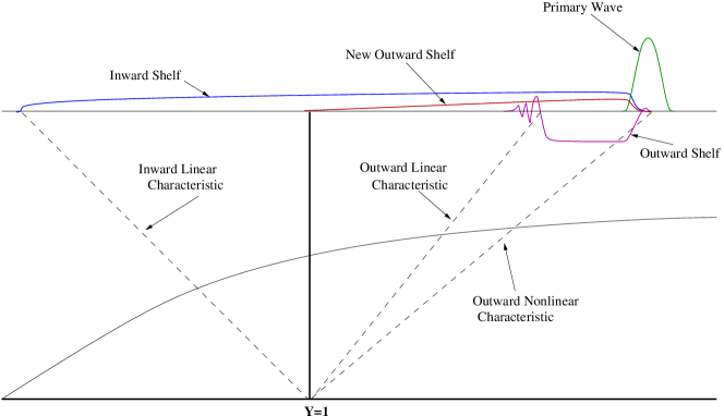
Figure 2: Schematic of Components in problem

4.1 Primary Wave

Equation (11) is a variable coefficient KdV equation; thus our $\operatorname{sech}^{2}$ initial profile is an exact solution for general $S(Y)$, however, in our particular problem we require $S(Y)=D^{-5/2}(Y)Y^{-2/3}$, in order to remove nonuniformities; this, along with the requirements of conservation of momentum, yields a solution for the primary wave as

$$H_{00}=\frac{A_{0}}{DY^{2/3}}\operatorname{sech}^{2}\left(\frac{\sqrt{3A_{0}}}{2D^{3/2}Y^{1/3}}\left(\xi-cX\right)\right),$$ (15)

where $A_{0}$ is the initial amplitude (at $Y=1$) of the wave.

4.2 Outward ’Shelf’

Now let us consider (12); we anticipate that, as this equation has distinct similarities to that of the plane-wave case, the solution to this equation will exhibit shelf-like properties.

Let us introduce $\phi=\xi-cX$, to be a characteristic moving with the primary wave (with $c$ the constant speed in $(\xi,X)$ space), and let $\phi=0$ be the peak. To demonstrate that the component $H_{01}$ does not approach zero near the tail of the primary wave, we construct an integral across a neighbourhood of $\phi=0$. This shows that

$$Z_{01}(T)=-\frac{m_{0}\bar{D}^{7/4}\bar{Y}^{1/6}}{c}(\bar{D}^{3/4}\bar{Y}^{1/6})_{T},$$

is the amplitude of $H_{01}$ directly behind the primary wave. Here we have defined $Y=\bar{Y}(T)$ to be $\phi=0$, describing the path of the primary wave.

From (12) we can also obtain a complete description of this wave component behind the primary wave. When we note that $H_{00}$ is exponentially small in its tails, we find that defining $H_{01}=D^{-1/4}Y^{-1/2}G_{01}$, then

$$G_{01}\sim\mathcal{G}^{\prime}\left(\sigma\phi+c\int\limits_{0}^{T}\bar{D}^{-2}\bar{Y}^{-2/3}dT\right),$$

where

$$\mathcal{G}(\mathcal{T})=-m_{0}\bar{Y}^{1/6}\bar{D}^{3/4}+\mathcal{A}\qquad\bar{Y}=\bar{Y}(\mathcal{T}),\bar{D}=\bar{D}(\mathcal{T}),$$

and

$$\mathcal{T}=c\int\limits_{0}^{T}\bar{D}^{-2}\bar{Y}^{-2/3}dT.$$

At the front (outside end) there exists a transition region (a region where transition back to undisturbed conditions occurs) around $\phi=0$; similarly, at the rear (inside end), a transition region exists around $\xi=0$. The detailed structure of these transitions can be obtained from (12) by considering the relevant asymptotic regions. They turn out to be, at the front,

$$H_{01}=D^{9/4}Y^{1/6}\left(D^{3/4}Y^{1/6}\right)_{Y}L\ ,$$

where

$$L= \frac{8}{3\sqrt{3}}{A_{0}}^{-5/2}\left\{\frac{3{A_{0}}^{2}}{2}(\tanh\theta-1)+\left(3{A_{0}}^{2}\theta+\frac{9{A_{0}}^{2}}{2}\right)\operatorname{sech}^{2}\theta\right.$$

$$\hskip 85.35826pt\left.-\tanh\theta\operatorname{sech}^{2}\theta\left(\frac{9{A_{0}}^{2}\theta}{2}+\frac{\hat{s}}{2}+3{A_{0}}^{2}\theta^{2}\right)\right\},$$

with

$$\theta=\frac{\sqrt{3A_{0}}}{2D^{3/2}Y^{1/3}}\left(\xi-cX\right),\qquad\hat{s}=\mathrm{constant};$$

and at the rear

$$H_{01}=D^{-1/4}Y^{-1/2}\mathcal{G}^{\prime}(0)\left\{1-\int^{\infty}_{x}Ai(u)du\right\};\quad x=\frac{\xi}{DY^{2/9}}\left(\frac{2}{X}\right)^{1/3}.$$

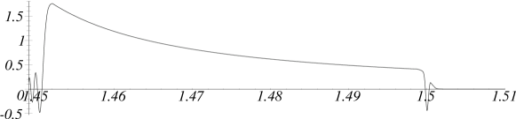
Figure 3: An example of the outward shelf behind the primary wave ($H_{01}$ against $Y$) using $A_{0}=1$, $\sigma=0.01$, $\Delta=0.1$ and $\bar{Y}=1.5$.

In Fig(3) we show a solution for the outward shelf combining the above expressions. We have made use of a simple depth profile, as an example ($D(Y)=Y^{-2}$), and have made necessary choices for the parameters and constants, which allow the three asymptotic solutions to be suitably joined at this order of approximation.

4.3 Mass Conservation

As we have already mentioned, the specific nature of this problem leads to an underlying requirement for global conservation of mass. After the application of all of the relevant scalings we obtain the mass conservation condition as

$$\int\limits_{0}^{\infty}H(R,\tau)R\textrm{d}R = \int\limits_{0}^{\infty}(H_{00}+\sigma H_{01}+\Delta H_{10}+\Delta\sigma H_{11}+\ldots)R\textrm{d}R$$

$$= \mathrm{Constant}.$$

Now let us consider the mass carried by the primary wave; this turns out to be

$$\int\limits_{0}^{\infty}H_{00}R\textrm{d}R\sim\bar{D}^{1/2}\bar{Y}\int\limits_{-\infty}^{\infty}H_{00}\textrm{d}\phi={m_{0}\bar{D}}{\bar{Y}^{2/3}},$$

a quantity which is clearly not constant. Thus the resulting difference from the initial O(1) mass, $m_{0}$, must be carried by other wave components.

We can calculate the mass carried by the Outward Shelf as

$${\sigma}\int\limits_{0}^{\infty}H_{01}(\xi,X,R)R\textrm{d}R\sim m_{0}\left({\bar{D}^{1/4}}{\bar{Y}^{1/2}}-{\bar{D}}{\bar{Y}^{2/3}}\right),$$

which satisfies the condition that the mass carried by this component is zero at $Y=1$. We can see that the total mass carried by these two components is

$$\int\limits_{0}^{\infty}(H_{00}+\sigma H_{01})R\textrm{d}R={m_{0}\bar{D}^{1/4}}{\bar{Y}^{1/2}}+O(\Delta),$$

Thus there must be other components carrying $O(1)$ mass.

4.4 Re-reflected Shelf

Let us now investigate the mass carried by the outward moving component of $H_{11}$. (We have written the non-local contributions to $H_{11}$ as $h_{11}+\Lambda_{11}$; see (13),(14).) This component is governed by (14) which can be integrated to yield

$$h_{11\xi}=-\frac{1}{2}D^{-1/4}Y^{-1/2}\int\limits_{1}^{Y}D^{-1/4}Y^{-1/2}\frac{\partial}{\partial Y}\left\{DYH_{00Y}\right\}dY.$$

For general depth profiles we are unable to obtain an explicit description for this wave component. However, the use of a specific form for the depth change, namely

$$D(Y)=\frac{(\beta+\gamma Y^{2})^{4/3}}{Y^{2}},$$ (16)

enables us to completely solve this equation and thereby elucidate some properties of this component.

Calculating the mass carried by this component, $M_{0}$, we now find that

$$M_{0} = {m_{0}}\int\limits_{1}^{\bar{Y}}\left[\frac{2\gamma(\beta+\gamma Y^{2})^{2/3}}{Y^{4/3}}-\frac{4(\beta+\gamma Y^{2})^{4/3}}{3Y^{7/3}}\right.$$

$$\hskip 85.35826pt+\left.\left(\frac{4}{3}-2\gamma\right)Y(\beta+\gamma Y^{2})^{-1/3}\right]dY.$$

4.5 Reflected Shelf

This component is governed by the pair of linear homogeneous equations (13). In order that we have conserved $O(1)$ mass, this component must be carrying the mass

$$m_{0}-{m_{0}\bar{D}^{1/4}}{\bar{Y}^{1/2}}-M_{0},$$

and this requirement uniquely determines $\Lambda_{11}$. The details are involved, but readily accessible (at least for suitable $D(Y)$).

The full solutions for both the reflected and the re-reflected shelves, for our specific choice for the depth profile (16), are not presented here; but they can be seen, along with the description of the transitions regions for the re-reflected shelf, in [9].

5 Conclusions

In this work we have presented a description of the wave components in cylindrical geometry that carry $O(1)$ mass. It has, however, not been possible to present all the details for general depth profiles (which would have been preferable). Nevertheless, we have shown the development of the method of solution, and from this can obtain some particular results.

Thus, for example, we find that if the depth profile takes certain (very simple) profiles, e.g. $D(Y)\propto Y^{-2/9}$, then one of the wave components, the new outward (re-reflected) shelf, will be absent.

One fundamental question which still has to be answered, concerns the behaviour of the inward (reflected) wave component. It is obvious, by the very nature of the problem, that any component propagating inwards will eventually reach the centre. There will undoubtably be some form of singularity at the centre, but there may be some choice for the depth profile in the neighbourhood of $r=0$ which will result in a particularly simple structure. The details of this investigation are still being developed, and may provide an impetus for further study.

References

- [1] F Calogero and A Degasperis. Solution by spectral transform method of a nonlinear evolution equation including as a special case the cylindrical KdV equation. Lett. Nuovo Cimento, 23:150–154, 1978.
- [2] R Hirota. Exact solutions to the equation describing “cylindrical solitons”. Phys. Lett., 71A(5,6):393–394, 1979.
- [3] R S Johnson. On the developemnt of a solitary wave moving over an uneven bottom. Proc. Camb. Soc., 73:183–203, 1973.
- [4] R S Johnson. On the inverse scattering transform, the cylindrical KdV equation and similarity solutions. Phys. Lett. A, 72:197–199, 1979.
- [5] R S Johnson. Water waves and the Korteweg-de Vries equation. J. Fluid Mech., 97:701–719, 1980.
- [6] R S Johnson. Ring waves on the surface of shear flows: A linear and non-linear theory. J. Fluid Mech., 215:145–160, 1990.
- [7] R S Johnson. Solitary wave, soliton and shelf evolution over variable depth. J. Fluid Mech., 276:125–138, 1994.
- [8] R S Johnson. A note on an asymptotic solution of the cylindrical Korteweg-de Vries equation. Wave Motion, 30:1–16, 1999.
- [9] S M Killen. Propagation of Nonlinear Water Waves over Variable Depth in Cylindrical Geometry Ph.D Thesis, Department of Mathematics, University of Newcastle Upon Tyne, 2000.
- [10] C J Knickerbocker and A C Newell. Shelves and the Korteweg-de Vries equation. J. Fluid Mech., 98, 1980.
- [11] C J Knickerbocker and A C Newell. Reflections from solitary waves in channels of decreasing depth. J. Fluid Mech., 153:1–16, 1985.
- [12] D J Korteweg and G de Vries. On the change of form of long waves advancing in a rectangular canal, and on a new type of long stationary wave. Phil. Mag., 39(5):422–443, 1895.
- [13] S Maxon and J Viecelli. Cylindrical Solitons. Phys. Fluids, 17:1614–1616, 1974.
- [14] J W Miles. On the Korteweg-de Vries equation for a gradually varying channel. J. Fluid Mech., 91(1):181–190, 1979.
- [15] A Nakamura and H H Chen. Soliton solutions of the cylindrical KdV equation. J. Phys. Soc. Japan, 50:711–718, 1981.
- [16] P M Santini. Asymptotic behaviour (in ) of solutions of the cylindrical KdV equation - I. Nuovo Cimento A, 54(2):241–258, 1979.
- [17] P M Santini. Asymptotic behaviour (in ) of solutions of the cylindrical KdV equation - II. Nuovo Cimento A, 57(4):387–396, 1980.