Tunable front interaction and localization of periodically forced waves

Abstract

In systems that exhibit a bistability between nonlinear traveling waves and the basic state, pairs of fronts connecting these two states can form localized wave pulses whose stability depends on the interaction between the fronts. We investigate wave pulses within the framework of coupled Ginzburg-Landau equations describing the traveling-wave amplitudes. We find that the introduction of resonant temporal forcing results in a new, tunable mechanism for stabilizing such wave pulses. In contrast to other localization mechanisms the temporal forcing can achieve localization by a repulsive as well as by an attractive interaction between the fronts. Systems for which the results are expected to be relevant include binary-mixture convection and electroconvection in nematic liquid crystals.

I Introduction

Localized structures have been observed in a range of pattern-forming nonequilibrium systems. One type of localized structure occurs when one pattern is embedded within another pattern. Examples include the coexisting stationary domains of long and short wavelengths observed in Taylor-Couette flow between co-rotating cylinders [1], in Rayleigh-Bénard convection in narrow slots [2], and in parametrically excited waves in ferrofluids [3]. Solitary waves drifting through a stationary pattern are found associated with a parity-breaking bifurcation in directional solidification [4], the printer instability [5], viscous fingering [6], cellular flames [7], and Taylor-vortex flow [8].

In this paper, we investigate a class of localized states in which the pattern is confined to a small region that is surrounded by the unpatterned state, or vice versa. For example, solitary standing waves (‘oscillons’) have been observed in vertically vibrated granular layers [9] and colloidal suspensions [10]. Localized traveling waves have been observed as one-dimensional pulses in binary-fluid mixtures [11, 12, 13, 14, 15] and as two-dimensional ‘worms’ in electroconvection of nematic liquid crystals [16].

For a general understanding of such structures the mechanisms that are responsible for their localization are of particular interest. A number of different types of localization mechanisms have been identified (e.g. [17]). To provide a context for our results we briefly review the main mechanisms.

The stable coexistence of domains of long and short wavelengths can be understood to be due to the instability of the constant wavenumber state combined with the conservation of the phase [18, 19, 20, 21, 22]. Localized patterns can also be stabilized by a non-adiabatic pinning of the large-scale envelope to the underlying small-scale pattern [23, 24]. This pinning has been suggested as a possible localization mechanism for oscillons [25].

To understand the traveling-wave pulses in binary mixture convection, two mechanisms have been put forward, dispersion [26, 27, 28] and the advection of a slowly decaying concentration mode [29, 30, 31, 32]. Within the framework of the complex Ginzburg-Landau equation with strong dispersion, pulses and holes can be viewed as perturbed bright and dark solitons of the nonlinear Schrödinger equation [33, 34, 35]. For weak dispersion, pulses have been described as a pair of bound fronts. In the absence of dispersion they are unstable. However, dispersion may result in a repulsive interaction between the two fronts and a stable pulse can arise [27, 28]. Similarly, the advected mode modifies the interaction between fronts and can also provide a stabilizing repulsive interaction. A similar advective mechanism has been invoked [36] to explain the two-dimensional localized waves (‘worms’) that have been observed in electroconvection in nematic liquid crystals [16].

More generally, the coupling of a pattern to an additional undamped (or weakly damped) mode can lead to its localization [37]. In the drift waves arising from a parity-breaking bifurcation, the local wavenumber of the underlying pattern plays the role of the additional mode [38, 39]. For the oscillons in vibrated granular media it has been suggested that a coupling of the surface wave to a mode representing the local height of the granular layer is important [40].

For traveling waves it is well known that the external application of a resonant temporal forcing excites the counter propagating wave [41, 42, 43]. A natural question is therefore whether the counterpropagating wave can play a role similar to the various additional modes mentioned above and can thus lead to the localization of the traveling wave into a pulse. Since the temporal forcing is easily controlled externally this localization mechanism would be tunable.

In this paper we investigate the effect of time-periodic forcing on spatially localized waves that arise in systems exhibiting a subcritical bifurcation to traveling waves as is, for instance, the case in binary-mixture convection. We expect the results also to be relevant for the worms observed in electroconvection in nematic liquid crystals.

We first consider the effect of forcing on the interaction of fronts in the absence of other localization mechanisms and show that forcing alone can lead to localized structures. This new localization mechanism can stabilize pulses with either a repulsive or an attractive interaction. While the interaction strength between fronts is usually determined by the system parameters, forcing allows the strength to be controlled externally. To focus on the interaction of the fronts due to the temporal forcing, we start in Section II with two coupled dispersionless Ginzburg-Landau equations and derive evolution equations for the fronts. In Section III we discuss the resulting front equations and compare them with numerical calculations. Section IV extends the analysis and discussion to include holes and multiple pulses. The combined effect of temporal forcing and dispersion is investigated in Section V and conclusions are presented in Section VI.

II Derivation of the front equations

Motivated by the pulses observed in binary mixture convection [11, 12, 13, 14, 15] and the worms in electroconvection [16] we consider a subcritical bifurcation to traveling waves in a one-dimensional system that is parametrically forced. To obtain a weakly nonlinear description, physical quantities like the temperature ${\cal T}$ of the fluid in the midplane in convection, say, are expanded in terms of the amplitudes $A$ and $B$, of the left and right traveling waves,

$${\cal T}=\epsilon^{1/2}\left\{A(x,t)e^{i(q_{c}\tilde{x}-\frac{\omega_{e}}{2}\tilde{t})}+B(x,t)e^{-i(q_{c}\tilde{x}+\frac{\omega_{e}}{2}\tilde{t})}\right\}+c.c.+h.o.t.,\qquad\epsilon\ll 1,$$ (1)

where $\tilde{t}$ and $\tilde{x}$ are the fast time and space coordinates. The amplitudes $A$ and $B$ are allowed to vary on a slow time scale $t$ and a slow spatial scale $x$. Due to the external periodic forcing $\epsilon^{2}\,\nu e^{i\omega_{e}\tilde{t}}$ close to twice the Hopf frequency, $\omega_{e}=2(\omega_{h}+\epsilon^{2}\Omega)$, the expansion (1) is chosen in terms of the forcing frequency. The forcing excites the oppositely traveling waves and breaks the time translation symmetry, resulting to lowest order in a linear coupling between the two wave amplitudes. Using the remaining spatial translation and reflection symmetries of the system, the form of the amplitude equations for $A$ and $B$ can be derived [41, 42, 43]. Hence we study the following set of coupled Ginzburg-Landau equations as a model describing the system,

$$\partial_{t}A = -s\partial_{x}A+\epsilon^{2}d_{2}\partial_{xx}A+\mu A+c|A|^{2}A-p|A|^{4}A$$ (3)

$$-g|B|^{2}A-r|A|^{2}|B|^{2}A-u|B|^{4}A+\nu B^{*}$$

$$\partial_{t}B = +s\partial_{x}B+\epsilon^{2}d_{2}\partial_{xx}B+\mu B+c|B|^{2}B-p|B|^{4}B$$ (5)

$$-g|A|^{2}B-r|A|^{2}|B|^{2}B-u|A|^{4}B+\nu A^{*},$$

where the forcing coefficient $\nu$ and the group velocity $s$ are real. All other coefficients may be complex. However, to focus on the interaction of the fronts due to temporal forcing, the front equations are derived for the case in which all of the coefficients are real, i.e. neglecting dispersion and detuning. Nonlinear gradient terms which would also appear in equations (3) and (5) to the order considered have also been neglected. In order for the bifurcation to be weakly subcritical, the cubic coefficients must be small enough to allow a balance with the quintic terms.

The bifurcation to spatially extended traveling waves in electroconvection in nematic liquid crystals appears to be supercritical [44]. To explain the observation of worms already below the onset of spatially extended waves, it has been argued that a weakly damped mode is relevant that is advected by the wave [36]. Already below threshold such a mode can lead to the existence of infinitely long worms, i.e. to convection structures that are narrow in the $y$-direction, say, and spatially periodic in the $x$-direction [36, 17]. They are expected to arise in a secondary bifurcation off the spatially extended traveling waves [45]. Focusing on the dynamics of the worms in the $x$-direction, the head and the tail of the worms can be considered as leading and trailing fronts that connect the nonlinear state, which is strongly localized in the $y$-direction, with the basic non-convective state. It is reasonable to expect that Ginzburg-Landau equations for a subcritical bifurcation will capture the qualitative aspects of these structures.

With the usual scaling $x=\epsilon\tilde{x}$ complex Ginzburg-Landau equations are obtained in which the growth term $\mu A$ is balanced by the diffusive term $d\partial_{xx}A$. For group velocities of order 1 this implies that the term $s\partial_{x}A$ is inconsistent with the rest of the equation, i.e. it is of lower order. However, by considering slower spatial scales $x=\epsilon^{2}\tilde{x}$, the advective term $s\partial_{x}A$ is of the same order as $\mu A$ and the diffusive term then appears in the re-scaled equations (3) and (5) as a higher-order correction of ${\cal O}(\epsilon^{2})$ as indicated in (3) and (5) [46].

We are interested in localized solutions made up of two bound fronts connecting the basic state with the nonlinear state as sketched in Figure 1. One contribution to the interaction between the fronts arises from their overlap. For large distances it is small, inducing a weak attractive interaction, which destabilizes pulses. However, since the diffusion is weak (${\cal O}(\epsilon^{2})$), resulting in steep fronts in A, the overlap between the fronts is of higher order in $\epsilon$ and the associated interaction can be ignored. Hence the interaction between the fronts is dominated by the presence of the oppositely traveling wave excited by the periodic forcing. The small diffusion coefficient causes internal layers to arise at the positions of the fronts. The two bound fronts are then divided into the five regions sketched in Figure 1, where $x_{L}$ and $x_{R}$ give the positions of the left and right fronts. Within regions I, III, and V the amplitude of $A$ is constant. Regions II and IV are regions of rapid change where the dynamics of the fronts are determined. The internal layers have a width $\Delta x={\cal O}(\epsilon)$, implying $\Delta\tilde{x}=\epsilon^{-2}\Delta x={\cal O}(\epsilon^{-1})$, which is still large relative to the critical wavelength of the traveling waves.

We consider the forcing to be small, $\nu={\cal O}(\epsilon)$, so that the corresponding amplitude $B$ of the left-traveling wave that is excited by the forcing is of the same order in $\epsilon$. The amplitudes and the parameters $\mu$ and $\nu$ are expanded as

$$A=A_{0}+\epsilon A_{1}+\cdots, \hskip 36.135ptB=\epsilon B_{1}+\cdots,$$ (6)

$$\mu=\mu_{c}+\epsilon^{2}\mu_{2}+\cdots, \hskip 36.135pt\nu=\epsilon\nu_{1}+\cdots.$$ (7)

where $\mu_{c}=-3c^{2}/16p$ is the value of the control parameter at which a single, non-interacting front is stationary. For $\mu>\mu_{c}$ the nonlinear convective state invades the basic state. In the following derivation we go into a reference frame moving with the group velocity $s$. The positions $x_{R}$ and $x_{L}$ of the right and left fronts evolve then on a slow time scale, $T=\epsilon^{3}t$.

Inserting the expansions (6) and (7) into equations (3) and (5) we obtain at leading order equations for $A$ and $B$ in the outer regions I, III, and V,

$$0 = \mu_{c}A_{0}+cA_{0}^{3}-pA_{0}^{5},$$ (8)

$$0 = 2s\partial_{x}B_{1}+\mu_{c}B_{1}+\nu_{1}A_{0}-gA_{0}^{2}B_{1}-uA_{0}^{4}B_{1}.$$ (9)

Solving equation (8) results in $A_{0}=0$ in regions I and V and $A_{0}^{2}=A_{c}^{2}\equiv 3c/4p$ in region III. The corresponding solution to (9) is

$$B_{1}^{j}(x)=\frac{\nu_{1}}{\alpha}A_{0}^{j}+K^{j}e^{\frac{\alpha^{j}}{2s}x},$$ (10)

where $j$ corresponds to the regions I, III, and V and $\alpha^{j}=-\mu_{c}+g(A_{0}^{j})^{2}+u(A_{0}^{j})^{4}$.

In the inner regions II and IV, the solutions vary on a fast space scale $x/\epsilon$ which is captured by introducing the inner coordinates $\eta=(x-x_{L})/\epsilon$ and $\eta=(x_{R}-x)/\epsilon$, respectively. The spatial derivative then transforms as $\partial_{x}\rightarrow\pm\partial_{\eta}/\epsilon$. The resulting leading-order equations for $A$ and $B$ are

$$0 = d_{2}\partial_{\eta\eta}A_{0}+\mu_{c}A_{0}+cA_{0}^{3}-pA_{0}^{5},$$ (11)

$$0 = \pm 2s\partial_{\eta}B_{1}.$$ (12)

From (11) one obtains the left and right front solution

$$A_{0}(\eta)=A_{c}\sqrt{\frac{1}{2}\left[1+\tanh{\left(\frac{\eta}{\xi}\right)}\right]},\;\;\;\;\;\;\xi=\frac{4}{c}\sqrt{\frac{pd_{2}}{3}},$$ (13)

where $A_{c}^{2}$ and $\eta$ are defined above. Equation (12) implies that $B_{1}$ does not depend on the fast space variable $\eta$, i.e. $B_{1}=B_{c}^{I,IV}$ is constant in regions II and IV. At ${\cal O}(\epsilon)$, no inhomogeneity arises in the equation for $A_{1}$, which is therefore taken to be identically $0$. But at ${\cal O}(\epsilon^{2})$ the following equation for $A_{2}$ is obtained:

$${\cal L}A_{2}=\mp\frac{dx_{L,R}}{dT}\partial_{\eta}A_{0}-\mu_{2}A_{0}+gB_{1}^{2}A_{0}+rA_{0}^{3}B_{1}^{2}-\nu_{1}B_{1},$$ (14)

where ${\cal L}=d_{2}\partial_{\eta\eta}+\mu_{c}+3cA_{0}^{2}-5pA_{0}^{4}$ is the linearized operator. It is singular and has the zero-eigenmode $\partial_{\eta}A_{0}$, which leads to a solvability condition for equation (14). The result of projecting equation (14) onto the zero-eigenmode determines the velocity of the fronts in regions II and IV,

$$\pm\frac{dx_{L,R}}{dT}=\left[-2\mu_{c}+(2g+A_{c}^{2}r)B_{c}^{II,IV^{2}}-\frac{4\nu_{1}B_{c}^{II,IV}}{A_{c}}\right]\xi$$ (15)

with $B_{c}^{II,IV}$ yet undetermined.

Since $B$ is generated by $A$, we consider the case where $B=0$ ahead of the pulse (i.e. for a right-traveling pulse region V where $A\equiv 0$). This implies that $K^{V}=0$ from equation (10). Now matching the inner and outer solutions for $B$ at the left and right positions ($x_{L}$ and $x_{R}$) of the fronts, one obtains the constant values $B_{c}^{II}=(\nu_{1}A_{c}/\alpha)\left[1-\exp{(-\alpha L/2s)}\right]$ and $B_{c}^{IV}=0$. The constants $K^{I}$ and $K^{III}$ are nonzero and we see from equation (10) that $B$ grows spatially to the left in region III and approaches the limiting value $\nu_{1}A_{c}/\alpha$. Then, in region I where the pulse has passed and $A$ again equals $0$, $B$ decays exponentially to zero. The individual front velocities are given by substituting the values of $B_{c}^{II,IV}$ into the expressions given in (15)

$$\frac{dx_{L}}{dT} = \left[-2(\mu-\mu_{c})+\frac{\nu^{2}(2g+A_{c}^{2}r)A_{c}^{2}}{\alpha^{2}}-\frac{4\nu_{1}^{2}}{\alpha}\right]\xi,$$ (16)

$$\frac{dx_{R}}{dT} = +2(\mu-\mu_{c})\xi.$$ (17)

Combining these results yields the following equations describing the evolution of the pulse length $L=x_{R}-x_{L}$ and the velocity of the pulse relative to a frame moving with the group velocity $s$ in terms of a “center of mass” coordinate $M=(x_{R}+x_{L})/2$,

$$\frac{dL}{dT} = k_{1}(\mu-\mu_{c})+k_{2}\nu^{2}(1-e^{-\frac{\alpha}{2s}L})-k_{3}\nu^{2}(1-e^{-\frac{\alpha}{2s}L})^{2},$$ (18)

$$\frac{dM}{dT} = \frac{1}{2}\left[-k_{2}\nu^{2}(1-e^{-\frac{\alpha}{2s}L})+k_{3}\nu^{2}(1-e^{-\frac{\alpha}{2s}L})^{2}\right],$$ (19)

where $k_{1}=4\xi$, $k_{2}=4\xi/\alpha,$ and $k_{3}=[(2g+A_{c}^{2}r)A_{c}^{2}\xi]/\alpha^{2}$. While both $k_{1}\mbox{ and }k_{2}$ are always positive, $k_{3}$ may be either positive or negative. As will be seen in the next section, the sign of $k_{3}$ determines whether stable pulse solutions may exist. The interaction length is given by $2s/\alpha$.

III Discussion of Front Equations

The possible pulse solutions of (18) and (19) are more easily discussed in terms of the quantity $\Lambda\equiv\left[1-\exp{(-\alpha L/2s)}\right]$ which monotonically increases from zero to one as $L$ increases from zero to infinity. Equation (18) is then given by

$$\frac{1}{1-\Lambda}\cdot\frac{d\Lambda}{dT}=f(\Lambda)\equiv k_{1}(\mu-\mu_{c})+k_{2}\nu^{2}\Lambda-k_{3}\nu^{2}\Lambda^{2}.$$ (20)

Figure 2 depicts $f(\Lambda)$ for the two cases $\mu>\mu_{c}$ and $\mu<\mu_{c}$. For $k_{3}>0$ the parabola opens downward and the maximum occurs at $\Lambda=k_{2}/2k_{3}$, independent of forcing strength $\nu$. Fixed points $\Lambda_{0}$ are indicated where $f(\Lambda)=0$:

$$\Lambda_{0}=(1-e^{-\frac{\alpha}{2s}L_{0}})\equiv\frac{k_{2}\pm\sqrt{k_{2}^{2}+\frac{4(\mu-\mu_{c})k_{1}k_{3}}{\nu^{2}}}}{2k_{3}}$$ (21)

Pulses with $\Lambda=\Lambda_{0}$ are linearly stable if $f^{\prime}(\Lambda_{0})<0$. If $k_{3}<0$, the parabola is opening upward with the minimum at $\Lambda=k_{2}/2k_{3}<0$ so that $f^{\prime}(\Lambda)>0$ for all values of $\Lambda>0$. Hence for a stable pulse to exist it is necessary that $k_{3}>0$ and in this case corresponds to the upper branch of solutions (21). More precisely, stable pulses exist as long as $k_{3}>k_{2}/2$ with their length diverging for $k_{3}\rightarrow k_{2}/2$. Unless stated otherwise the discussion of the front interaction will focus on the regime $0<k_{2}/2k_{3}<1$ where a stable branch exists.

From the expression (21) and the parabola in Figure 2, one can easily see the effect of forcing on the stable pulse length. As the forcing $\nu$ increases, $f(\Lambda=0)=f(\Lambda=k_{2}/k_{3})=k_{1}(\mu-\mu_{c})$ remain fixed while the parabola steepens (see Figure 2). Thus for $\mu>\mu_{c}$ the stable pulse length is larger than $L_{c}$ corresponding to $\Lambda_{c}\equiv k_{2}/k_{3}$, but approaches $L_{c}$ as forcing increases (Figure 2a). Conversely, for $\mu<\mu_{c}$ the pulse length increases to $L_{c}$ with increasing $\nu$ (Figure 2b). As forcing $\nu$ decreases for $\mu>\mu_{c}$, the pulse length increases and eventually diverges to infinity. In contrast, for $\mu<\mu_{c}$ decreasing forcing results in the pulse length decreasing until the pulse is destroyed in a saddle-node bifurcation.

Figure 3 shows both the analytical results for the steady state solutions of equation (18) and numerical results obtained by integrating the full amplitude equations (3) and (5). A linearized Crank-Nicholson scheme was used to solve the coupled equations and the pulse lengths were measured at half-amplitude. The pulse length is plotted as a function of forcing strength for several values of the control parameter $\mu$ confirming the expected behavior. The top figure is for group velocity $s=20.0$ and the bottom figure for $s=1.7$. Here we see that although the analytical result no longer agrees quantitatively for smaller $s$, it still describes the qualitative behavior of the pulse length as the control parameters are varied. This dependence on the group velocity will be discussed at the end of this section.

A numerical control technique has been employed to obtain the unstable pulse solutions indicated by the long dashed curves in Figure 3. Since the analysis leads to a single ordinary differential equation (18) describing the evolution of a pulse, the dynamics of the pulse length are essentially restricted to a one-dimensional manifold. The control technique is therefore relatively straight-forward. Pulse lengths are measured after evolving equations (3) and (5) over a short time interval and compared with the measurements taken at the previous time to obtain the direction and rate of growth. This information is then used along with the desired pulse length to adjust the control parameter accordingly. This process is repeated until a steady-state pulse with the specified length is obtained. In Figure 3, the parameter adjusted to control the length is the forcing strength $\nu$ while all other parameters remain fixed. The same technique is also used for varying the control parameter $\mu$ (cf. Figures 8b, 9, and 12).

The different regimes can be understood by looking at the individual interaction terms in equation (18) and their origins from equation (3). The first term in (18) is a measure of how far the control parameter $\mu$ is from the critical value $\mu_{c}$ where, in the absence of forcing, an isolated front is stationary. It provides a “pressure” which is directed outward for $\mu>\mu_{c}$ and which has to be balanced by the interaction terms. The second and third terms describe the interaction between fronts due to forcing. The second term arises from the linear coupling between $A$ and $B$ introduced by the forcing in equation (3) through which $B$ excites $A$. It therefore enhances the invasion of the nonlinear state into the linear state, which corresponds to a repulsive interaction between the leading and the trailing front. The third term stems from the nonlinear coupling which, when $k_{3}>0$, suppresses $A$ and therefore weakens the invasion, implying attraction between the fronts.

The effect of forcing on a pulse depends on the distance between the fronts. Since the pulse is traveling to the right, the amplitude $B$ is growing spatially to the left. For short pulses, therefore, $B$ remains small and the linear coupling term dominates the interaction implying a repulsive interaction. Thus, for $\mu<\mu_{c}$ the inward “pressure” can be balanced by a repulsive interaction if the pulses are sufficiently short. With increasing pulse lengths, $B$ reaches larger values at the trailing front and the nonlinear coupling term gains importance. Thus, in contrast to many other localization mechanisms, the forcing can induce an attractive interaction that grows with distance. It is able to balance the outward “pressure” for $\mu>\mu_{c}$. In this regime the pulses become shorter with increased forcing. Figure 4 shows two stable pulse solutions obtained by numerically integrating equations (3) and (5). The control parameter $\mu=-1.240$ for the longer pulse and $\mu=-1.250$ for the shorter pulse. All other parameters are the same for both pulses. Note that the forcing $\nu$ is the same for both pulses, yet the amplitude $B$ has not saturated for the shorter pulse.

From equations (18) and (19) we see that when $dL/dT\equiv 0$ for a steady pulse $L_{0}$, then $dM/dT=k_{1}(\mu-\mu_{c})/2$. Thus the pulse velocity in the moving frame is given by the invasion speed and depends on $\mu$. By contrast, in dispersively stable pulses the velocity depends on the control parameter only through the nonlinear gradient terms [27, 28]. Strikingly, in the asymptotic calculation leading to (19) the pulse velocity does not depend on the forcing $\nu$. Figure 5a shows that the linear dependence on $\mu$ is in good agreement with this analytical result, but that the velocity does also depend on forcing $\nu$. We suggest that the discrepancy may be explained by the effect of the excited counter-propagating wave on the leading front at $x_{R}$. Since in the weakly nonlinear regime diffusion is much weaker than advection (for group velocities of ${\cal O}(1)$), $B_{c}=0$ in region IV, which implies that forcing has no affect on the velocity of the leading front (equation 15). However, non-zero $B$ within this inner region will slightly alter the velocity of the leading front and consequently that of the pulse as a function of forcing. This will also impact the length of the pulse. For the parameters used in Figure 4, note that $B$ varies slowly in region II whereas it varies almost as fast as $A$ in region IV suggesting that the missing contribution is more prevalent at the leading front than at the trailing one. Figure 5b shows single front velocities for both the leading and trailing front. The curves are the analytical results obtained from (15) for single fronts ($L\rightarrow\infty$) and the symbols indicate numerical results. As expected, the velocity of the trailing front is well described by our analysis, but the velocity of the leading front does depend slightly on the forcing. The leading-front velocity then dictates the velocity of the pulse. For larger group velocity $s$, the interaction length $2s/\alpha$ increases and the separation of the fast and slow spatial scales at the positions of the fronts becomes more distinct, as shown in Figure 6. Thus we expect and the numerical results confirm (Figure 7) that the agreement with analytical results (18) and (19) for pulse length and velocity improves with increasing group velocity $s$. For small forcing $\nu$ the relative error of the velocity is on the order of the numerical accuracy. We note that the qualitative behavior of the pulse length is consistent even for smaller group velocity.

IV Holes and Multiple Pulses

The analysis from section II can be applied to other front configurations such as hole states and multiple pulses. A hole consists of a localized region in which the amplitude of the pattern is very small and which is surrounded by the nonzero traveling-wave amplitude. In contrast to the hole-type solutions found in the Ginzburg-Landau equation [35, 47], which are qualitatively different objects than pulses, the holes to be discussed here are similar to pulses in that they are also compound objects made of two fronts connecting the basic state with the nonlinear state. As with the pulses, the central equation for their description is an evolution equation for the length $L_{h}$ of the hole. It is given by

$$\frac{dL_{h}}{dT}=-k_{1}(\mu-\mu_{c})-k_{2}\nu^{2}(1+e^{-\frac{|\mu_{c}|}{2s}L_{h}})+k_{3}\nu^{2}(1+e^{-\frac{|\mu_{c}|}{s}L_{h}}),$$ (22)

where $k_{1},k_{2}$, and $k_{3}$ are defined as before and a stable hole may be possible when $k_{3}>0$. Note that the interaction length for holes is now given by $2s/|\mu_{c}|$ which is longer than the interaction length $2s/\alpha$ for pulses. Solving $dL_{h}/dT=0$ again yields two possible solutions $L_{h}^{\pm}$, with the longer hole unstable and the shorter hole stable. In contrast with the pulses, stable holes thus exist only over a finite range of shorter lengths. The RHS is quadratic in $\Lambda_{h}=\exp(-|\mu_{c}|L_{h}/2s)$, describing a parabola opening upward. Although varying forcing now results not only in stretching the parabola, but also in shifting it vertically, the variations in hole length again depends on the sign of the first term in (22). When $\mu<\mu_{c}$, increasing forcing causes stable holes to get shorter, while for $\mu>\mu_{c}$ the stable hole length will increase. Although the tendency of a hole to grow or shrink with increased forcing depends only on the sign of $\mu-\mu_{c}$, the limiting behavior is different depending on the relative sizes of $k_{2}$ and $k_{3}$. If $k_{3}<k_{2}$ then holes exist only for $\mu<\mu_{c}$ and as $\nu$ increases, the hole length goes to zero. If $k_{3}>k_{2}/2(\sqrt{2}-1)\approx 1.2k_{2}$, holes exist only for $\mu>\mu_{c}$ and as $\nu$ increases the stable hole length grows and eventually disappears in a saddle-node bifurcation with the unstable hole. Finally, for the intermediate values of $k_{3}$, holes exist for values of $\mu$ both above and below $\mu_{c}$. In this case, as $\nu\rightarrow\infty$, the hole length approaches the limiting length determined when $\mu=\mu_{c}$.

Figure 8a,b shows a stable numerical hole solution and the control parameter $\mu$ as a function of the hole length for different values of the forcing. Stable and unstable solutions are indicated by solid and open symbols, respectively. Again, the unstable holes are obtained by means of a numerical control technique. First we note that according to (22), the minimum of these curves should all be at the same value of $L_{h}$, but our numerical results show the minimum shifted to the right as $\nu$ increases. The analysis requires that $A$ vanish in the hole region, but the presence of $B$ in this region actually generates small nonzero $A$, which in turn generates $B$. Hence, the actual value of $B$ at the trailing front is greater than predicted. This suppresses $A$ there and the trailing front slows down, leading to longer pulses and a shift of the minimum of the curves to the right as forcing $\nu$ increases. If the parameters are such that the control parameter $\mu$ can be taken smaller, the basic state is more strongly damped. Hence, within the hole region $A$ is smaller and the shift of the curves is less pronounced as seen in Figure 9. Here $c=2.58$ so that $\mu_{c}\sim-1.248$ as compared to $c=1.8$ in Figure 8 where $\mu_{c}\sim-0.608$.

Arrays of multiple fronts can be combined to form multiple pulses. For a two-pulse configuration, there are four inner front regions which match to five outer regions resulting in evolution equations for the distance $L_{2}$ between the pulses as well as the widths $L_{1}$ and $L_{3}$ of the leading and the trailing pulse, respectively. This is to be contrasted with the description of multi-pulse solutions in the strongly dispersive case (without forcing), where the pulse widths can be adiabiatically eliminated in favor of the the distance and the phase difference between the two individual pulses [48]. The three evolution equations for $L_{1,2,3}$ are given by

$$\frac{dL_{1}}{dT} = k_{1}(\mu-\mu_{c})+k_{2}\nu^{2}\Lambda_{1}-k_{3}\nu^{2}\Lambda_{1}^{2},$$ (23)

$$\frac{dL_{2}}{dT} = -k_{1}(\mu-\mu_{c})-k_{2}\nu^{2}\Lambda_{1}(1+\Lambda_{2})+k_{3}\nu^{2}\Lambda_{1}^{2}(1+\Lambda_{2}^{2}),$$ (24)

$$\frac{dL_{3}}{dT} = k_{1}(\mu-\mu_{c})+k_{2}\nu^{2}\left\{\Lambda_{1}\Lambda_{2}+\left[1+\Lambda_{3}(\Lambda_{1}\Lambda_{2}-1)\right]\right\}$$ (26)

$$\;\;\;\;\;\;\;\;-k_{3}\nu^{2}\left\{\Lambda_{1}^{2}\Lambda_{2}^{2}+\left[1+\Lambda_{3}(\Lambda_{1}\Lambda_{2}-1)\right]^{2}\right\},$$

where the $\Lambda_{i}$ are defined in terms of $L_{i}$ as follows: $\Lambda_{1}=1-\exp(-\alpha L_{1}/2s),\Lambda_{2}=\exp(\mu_{c}L_{2}/2s)$, and $\Lambda_{3}=\exp(-\alpha L_{3}/2s)$. Since equation (23) for $L_{1}$ is the same as equation (18) which describes a single pulse, the leading pulse length is unaffected by the trailing pulse. But the trailing pulse length depends on both the length of the leading pulse and the distance between the pulses and is typically shorter than the leading pulse. Solving equations (23) and (26) for the fixed points $\Lambda_{10},\Lambda_{20},\Lambda_{30}$, it is found that $\Lambda_{10}\cdot\Lambda_{20}=k_{2}/k_{3}$ and $\Lambda_{30}=k_{3}\cdot(1-\Lambda_{10}/(k_{3}-k_{2})$. Since $L_{1}$ increases with increasing $\Lambda_{1}$, and $L_{2}$ and $L_{3}$ increase with decreasing $\Lambda_{2}$ and $\Lambda_{3}$, this suggests that all three lengths will either increase or decrease as the control parameters $\mu$ and $\nu$ are varied. The eigenvalues $\sigma_{i}$ obtained from linearizing equations (23) and (26) indicate that $\sigma_{1}=\sigma_{3}$ and a two-pulse solution may be stable when $k_{3}$ is positive. A stable two-pulse solution is therefore expected to exist and be stable whenever a single pulse exists. However, since the trailing pulse is narrower than the leading pulse, it may become too short and collapse - as it merges in a saddle-node bifurcation with the shorter unstable pulse - for parameter values where the single pulse is still stable. Numerically, we observe that as the control parameter $\mu$ is decreased all three lengths get shorter and the trailing pulse eventually collapses to zero. Figure 10 shows a stable two-pulse solution superimposed over a single pulse solution confirming that the leading pulse length is unaffected by the trailing pulse.

V Dispersion Effects

Waves generally have both linear and nonlinear dispersion. Hence, the coefficients and the amplitudes in equations (3) and (5) are in general complex. In [27, 28], it is shown that for weak dispersion the interaction between fronts leads to the following type of evolution equation for the length of a pulse:

$$\frac{dL}{dt}=k_{1}(\mu-\hat{\mu}_{c})-k_{4}e^{-L/\xi}+\frac{k_{5}}{L}.$$ (27)

The coefficients $k_{1}$ and $k_{4}$ are positive and contain only the real part of the original coefficients. The first term is similar to equation (18) where $\hat{\mu}_{c}$ is the value of the control parameter at which a single, isolated front is stationary. Due to the dispersive terms, $\hat{\mu_{c}}$ includes a correction compared to $\mu_{c}$. The second term arises as a result of the overlap of the fronts in the convective amplitude. The term involving $k_{5}$ contains the imaginary parts of the coefficients, so that this term represents the interaction due to dispersion. When $k_{5}>0$, dispersion provides a repulsive interaction and can lead to the existence of stable pulses. When $\mu<\hat{\mu}_{c}$ two pulse solutions exist with the longer one being stable.

We now consider the combined effects of forcing and dispersion. Of particular interest is the question whether periodic forcing can stabilize or destabilize pulses obtained in the purely dispersive regime. The task of deriving front equations including both dispersion and forcing seems formidable. It is suggested and validated by the numerical simulations below that the relevant aspects of both features may be modeled by simply adding the two contributions. This leads to an equation of the following form for pulses of length $L$:

$$\frac{dL}{dT}=k_{1}(\mu-\hat{\mu}_{c})+k_{2}\nu^{2}(1-e^{-\frac{\alpha}{2s}L})-k_{3}\nu^{2}(1-e^{-\frac{\alpha}{2s}L})^{2}-k_{4}e^{-L/\xi}+\frac{k_{5}}{L}.$$ (28)

If both dispersion and forcing independently result in a stable pulse, their combined contribution merely enhances the stability of the pulse. The case of competing contributions is more interesting. Figure 11 is a plot of the control parameter $\mu$ as a function of steady-state pulse lengths $L$ from equation (28). The dashed curve is for dispersion in the absence of forcing ($\nu=0$), whereas the solid and dotted curves indicate the addition of forcing. For a given value of the control parameter indicated by the thin horizontal line stable equilibrium solutions (positive slope) are given by solid circles while open circles indicate unstable solutions (negative slope). Plotted are both cases, a) when weak dispersion leads to a stable pulse, $k_{5}>0$, and b) when it does not, $k_{5}<0$. If forcing does not stabilize a pulse ($k_{2}/2k_{3}>1$), then increasing forcing pushes the stable branch of solutions downward. There is a competition between the two interactions and four solution branches may exist (Figure 11a inset). Eventually, for sufficiently large forcing $\nu$ the stable pulse disappears at infinity, leaving only the unstable pulse solution. Similarly, when dispersion does not stabilize the pulse, increasing forcing with $k_{2}/2k_{3}<1$ can eventually lead to a stable pulse branch (Figure 11b).

For large $L$, equation (28) is dominated by the dispersive interaction, which decays only like $1/L$, suggesting that the original, dispersive behavior is recovered for large lengths $L$. If $k_{2}/2k_{3}>1$ the competition can lead to two additional pulses, one unstable and one stable, for intermediate values of forcing $\nu$ (cf. inset of Fig. 11a). For larger forcing, only one unstable pulse and one long, stable pulse remain. Note that for fixed $\mu$ and increasing $\nu$ the stable pulse will still disappear at infinity since the branch is being pushed downward. If the forcing generates a stable pulse, the $1/L$-behavior of the dispersive interaction suggests the existence of a long, third, unstable pulse (Fig. 11b). Note that according to the analysis of the dispersive interaction in [27], which was confirmed numerically in [31], the power-law behavior continues only up to a maximal length $L_{max}$, beyond which the dispersive interaction decays rapidly. The maximal length $L_{max}$ decreases with increasing dispersion. If forcing dominates the interaction for lengths up to $L_{max}$, then the long-length dispersively dominated behavior is no longer expected for either case depicted in Figure 11. But it should be present for weaker forcing or shorter interaction length.

Figures 12 show numerical results that confirm the expected pulse behavior based on equation (28). Plotted are the numerically obtained pulse lengths as a function of the control parameter $\mu$. Stable pulse solutions are indicated by solid symbols and unstable solutions by open symbols. Figures 12a,b show that increased forcing may destroy a dispersively stable pulse. For forcing strength $\nu=0.2$, the forcing is not sufficient to eliminate the stable pulse and both solution branches are still present. The inset shows an intermediate value of $\nu=0.4$ where four solution branches exist and Figure 12b shows the pulse lengths for stronger forcing $\nu=0.5$, where only the unstable branch remains. Figures 12c,d depict the creation of a stable pulse branch by increasing forcing strength. When $\nu=0.1$ forcing leads to a stable branch, but for longer lengths the dispersion dominates and a third, unstable pulse exists. However, for $\nu=0.2$ the forcing succeeds in dominating the interaction beyond $L_{max}$ so that the branch remains stable.

VI Conclusions

In this paper we have investigated the effect of external resonant forcing on the interaction of fronts connecting the stable basic with a stable nonlinear traveling-wave state that arises in a subcritical bifurcation. Localized structures were described analytically as bound pairs of fronts. The temporal forcing excites the oppositely traveling wave and provides an additional mode that is sufficient to localize structures. Since the forcing constitutes an externally controlled parameter, pulses of tunable length can be obtained via this new localization mechanism. Forcing stabilizes pulses through either a repulsive or an attractive interaction between the fronts depending on the pulse length. This is in contrast to other localization mechanisms in which stable pulses arise only for a repulsive interaction [27, 28, 30]. Multiple pulses with different, but fixed, lengths and holes are also obtained. In addition, the combined effect of temporal forcing and dispersion has been investigated. With the inclusion of weak dispersion, the interaction between fronts can be described qualitatively by a single equation combining the two interaction terms (28). It was found that in the dispersive regime forcing can lead to the creation of new pulses or the destruction of pulses depending on system parameters. The competition between the two interactions determines the number and stability of pulses observed.

In the regimes investigated here no complex dynamics of the individual pulses have been found. It is known, however, that both dispersively stabilized pulses as well as pulses stabilized by an advected mode can undergo transitions to chaotic dynamics (e.g. [49, 50, 51]).

Localized traveling waves in the absence of resonant forcing have been observed experimentally in particular in binary-mixture convection and electroconvection in nematic liquid crystals. Depending on parameters, the localization of pulses in binary-mixture convection is understood to be due to dispersion and to the coupling to a slowly decaying, advected concentration mode. Since the advection depends on the direction of propagation of the wave, an interesting question is how the counterpropagating wave excited by a resonant forcing will affect the pulses that are stabilized by the concentration mode and how the two localization mechanisms interact. The origin of the localization of the worms in electroconvection is still being investigated. A Ginzburg-Landau model that includes a coupling to a weakly damped mode similar to that in the case of binary-mixture convection has been proposed [36]. By probing the response of the worms to temporal forcing, insight may be gained into the relevance of an advected mode in the worms.

We would like to acknowledge discussions with J. Viñals. This work has been supported by the Engineering Research Program of the Office of Basic Engineering Science at the Department of Energy under grant DE-FG02-92ER14303 and the National Science Foundation under grant DMS-9804673.

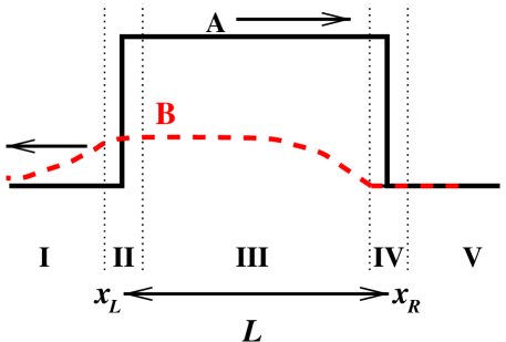
FIG. 1.: Sketch of a pulse traveling to the right. $A$ is the amplitude of the right-traveling wave. Temporal forcing excites the left-traveling wave $B$, which grows spatially to the left reaching a maximum at the trailing front, behind which it decays exponentially.

             

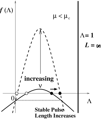
FIG. 2.: Sketch of $f(\Lambda)\equiv k_{1}(\mu-\mu_{c})+k_{2}\nu^{2}\Lambda-k_{3}\nu^{2}\Lambda^{2}$ for $k_{3}>0$. Stable (unstable) fixed points are indicated by solid (open) circles. Varying forcing changes the steepness of the parabola and the height of the maximum located at $\Lambda=k_{2}/2k_{3}$. Increasing forcing $\nu$ decreases the stable pulse length for (a) $\mu>\mu_{c}$ and increases the stable pulse length for (b) $\mu<\mu_{c}$.

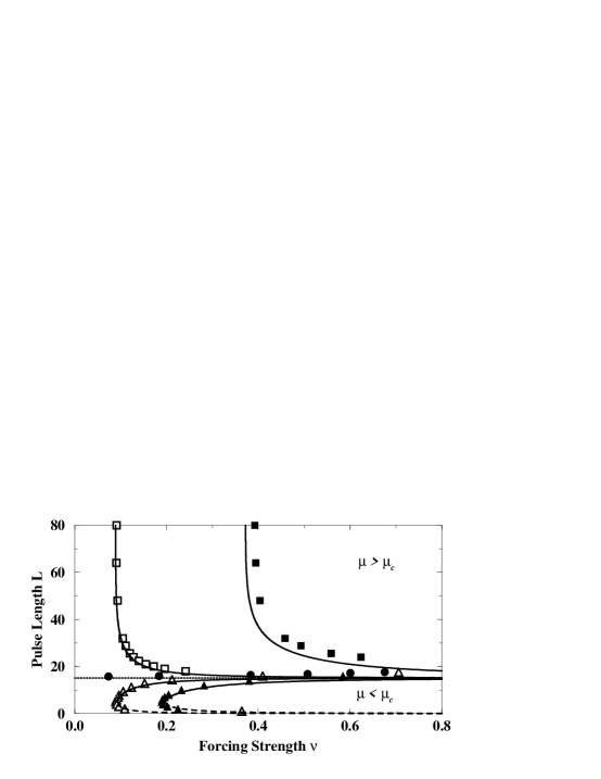
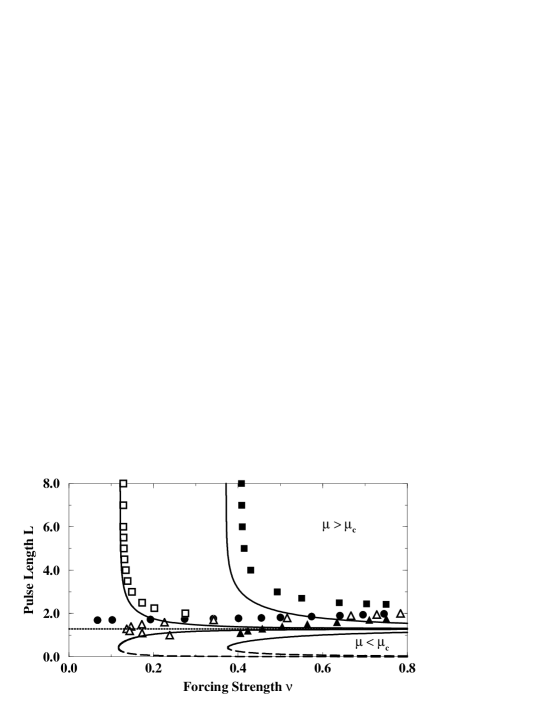
FIG. 3.: Dependence of pulse length $L$ on the forcing strength $\nu$. The symbols indicate the numerical results and the curves are obtained from equation (21). The dotted line corresponds to $\mu=\mu_{c}$. The curves above (below) this line correspond to values of $\mu>\mu_{c}$ ($\mu<\mu_{c}$). The dashed curves indicate unstable branches. The group velocity $s=20\mbox{ and }1.7$ in the top and bottom figures, respectively. $\mu=-1.238$ (solid squares), $-1.2475$ (open squares), $-1.248075=\mu_{c}$ (circles), $-1.2485$ (open triangles), and $-1.250$ (solid triangles). All other parameters are as in Figure 4.

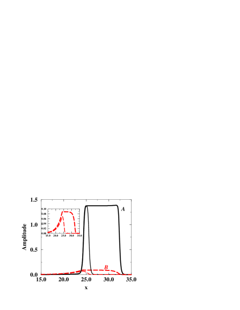
FIG. 4.: Numerically obtained long and short stable pulse solutions, with $\mu>\mu_{c}$ and $\mu<\mu_{c}$, respectively. The inset zooms in on the amplitude $B$ only. The parameters are $\nu=0.2534,s=1.7,d=0.05,c=2.58,p=1.0,g=1.4,r=4.0$, and $\mu=-1.244$ ($\mu=-1.250$) for the long (short) pulse. For these parameters $\mu_{c}=-1.248075$.

     

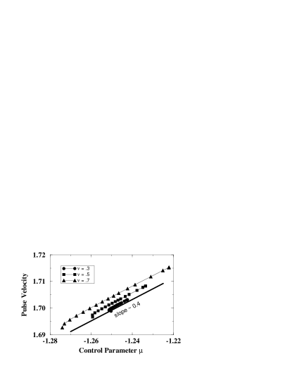
FIG. 5.: (a) Pulse velocity as a function of $\mu$ for forcing $\nu=0.3,0.5$, and $0.7$. The line shown is obtained from the analytical result $v_{pulse}=k_{1}(\mu-\mu_{c})/2+s$. (b) Velocity dependence on forcing $\nu$. The solid and open symbols indicate the numerically obtained velocities for the trailing and leading fronts, respectively. The curves give the analytical results. Squares are for $\mu=-1.250$ and circles for $\mu=-1.238$. The small symbols show the corresponding numerically obtained pulse velocities. All other parameters are as in Figure 4.

FIG. 6.: Amplitude $B$ of pulse solutions when $s=1.25,5.0,20.0$ indicated by the thick dotted, dashed, and solid lines, respectively. The amplitudes $A$ are indicated by thin lines and the leading front in $A$ is indistinguishable between the different velocities. $\mu=-1.2485,\nu=0.29$ and all other parameters as in Figure 4.

     

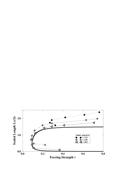
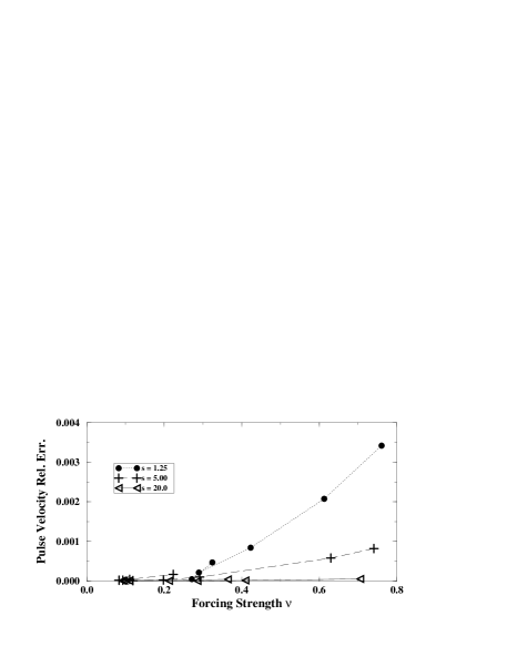
FIG. 7.: (a) Scaled pulse length and (b) relative error of pulse velocity versus forcing $\nu$ for $s=1.25,5.0,20.0$. $\mu=-1.2485$ and all other parameters as in Figure 4.

     

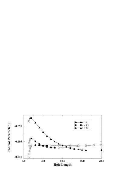
FIG. 8.: (a) Numerical hole solution for $c=1.8,\mu=-0.609$, and $\nu=0.3$. (b) Control parameter $\mu$ as a function of hole length for various values of $\nu$. For $c=1.8$, $k_{3}$ is in the regime where holes exist for both $\mu>\mu_{c}$ and $\mu<\mu_{c}$. Solid (open) symbols refer to stable (unstable) solutions. All other parameters are as in Figure 4 .

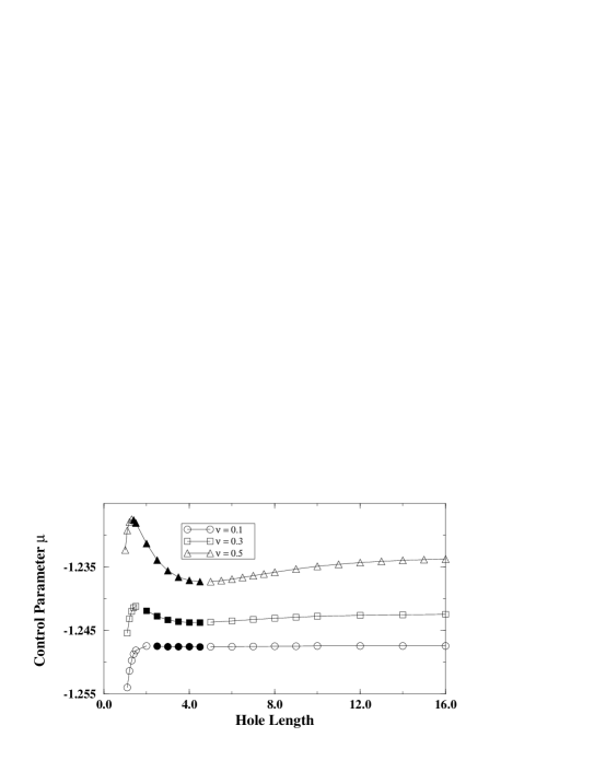
FIG. 9.: Control parameter $\mu$ as a function of hole length for various values of $\nu$. For $c=2.58$, $k_{3}$ is in the regime where stable holes exist only for $\mu>\mu_{c}$. Solid (open) symbols indicate stable (unstable) solutions. All other parameters are as in Figure 4 .

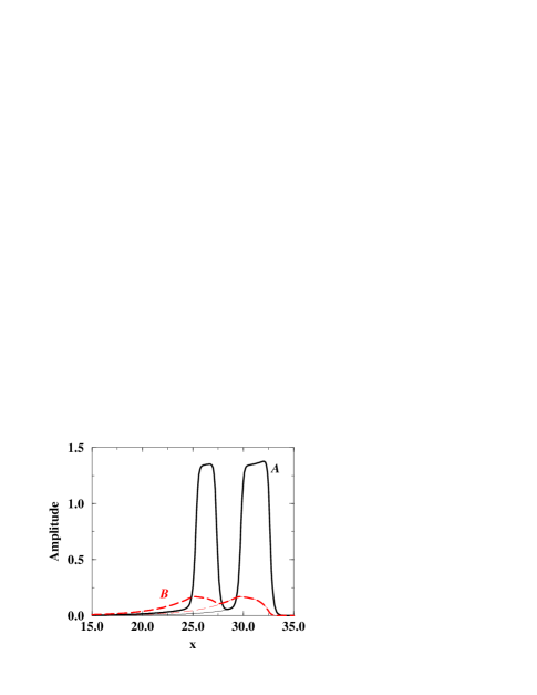
FIG. 10.: Two-pulse solution (thick lines) superimposed over a single-pulse solution (thin lines) for $\mu=-1.238,\nu=0.5$, and all other parameters as in Figure 4.

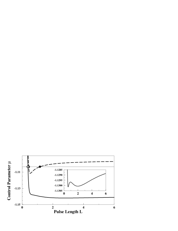
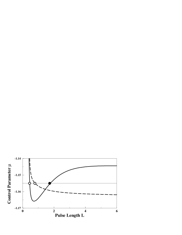
FIG. 11.: Control parameter $\mu$ vs. steady-state pulse lengths of equation (28) for dispersion only, $\nu=0$ (dashed curve), and added forcing, $\nu=0.5$ (solid curve). The solid circles indicate stable solutions (positive slope) and the open circles unstable ones (negative slope). (a) For $k_{5}>0$ and $k_{2}/2k_{3}>1$ forcing can eventually destroy a stable pulse, $d=0.01+0.0i,r=0.0$. The inset shows the four branches possible for an intermediate value of forcing $\nu=0.425$. (b) For $k_{5}<0$ and $k_{2}/2k_{3}<1$ increased forcing can lead to stable pulse solutions, $d=0.01-0.01i,r=4.0$. All other parameters are the same: $s=1.7,c=2.45+0.2i,p=1.0,g=1.4$.

     

     

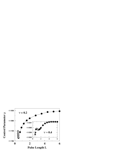
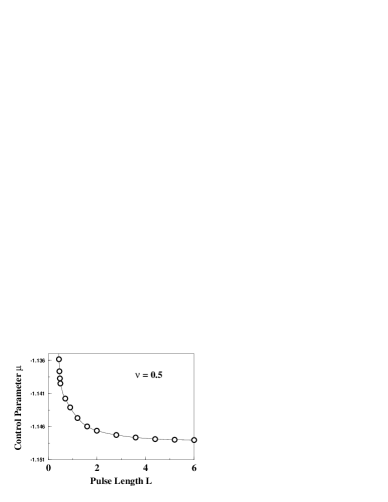
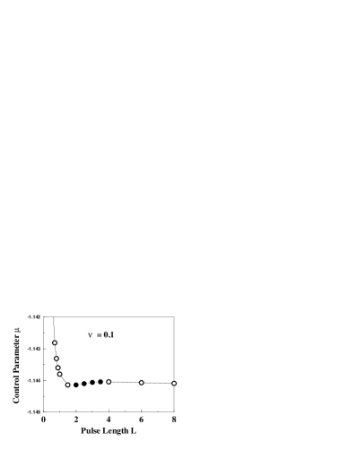
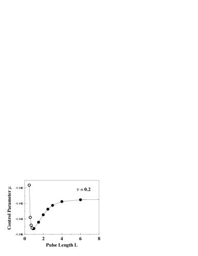
FIG. 12.: The control parameter $\mu$ vs. the pulse length L. Stable (unstable) solutions indicated by solid (open) symbols. Top row (a)-(b) Forcing destroys a dispersively stable pulse ($d=0.01+0.0i$ and $r=0.0$). Forcing strength $\nu=0.2$ and $\nu=0.4$ (inset) in (a), and $\nu=0.5$ in (b). Bottom row (c)-(d) Forcing creates a stable branch ($d=0.01-0.005i$ and $r=4.0$). Forcing strength $\nu=0.1$ in (c) $\nu=0.2$ in (d). All other parameters are the same: $s=1.7,c=2.45+0.2i,p=1.0,g=1.4$.

REFERENCES

- [1] B. Baxter and C. Andereck, Phys. Rev. Lett. 57, 3046 (1986).
- [2] J. Hegseth, J. Vince, M. Dubois, and P. Bergé, Europhys. Lett. 17, 413 (1992).
- [3] T. Mahr and I. Rehberg, Phys. Rev. Lett. 81, 89 (1998).
- [4] A. Simon, J. Bechhoefer, and A. Libchaber, Phys. Rev. Lett. 61, 2574 (1988).
- [5] M. Rabaud, S. Michalland, and Y. Couder, Phys. Rev. Lett. 64, 184 (1990).
- [6] H. Cummins, L. Fourtune, and M. Rabaud, Phys. Rev. E 47, 1727 (1993).
- [7] M. Gorman, M. el Hamdi, and K. Robbins, Comb. Sci. and Tech 98, 71 (1994).
- [8] R. Wiener and D. McAlister, Phys. Rev. Lett. 69, 2915 (1992).
- [9] P. Umbanhowar, F. Melo, and H. Swinney, Nature 382, 793 (1996).
- [10] O. Lioubashevski et al., Phys. Rev. Lett. 83, 3190 (1999).
- [11] E. Moses, J. Fineberg, and V. Steinberg, Phys. Rev. A 35, 2757 (1987).
- [12] P. Kolodner, D. Bensimon, and C. Surko, Phys. Rev. Lett. 60, 1723 (1988).
- [13] J. Niemela, G. Ahlers, and D. Cannell, Phys. Rev. Lett. 64, 1365 (1990).
- [14] P. Kolodner, Phys. Rev. Lett. 66, 1165 (1991).
- [15] P. Kolodner, Phys. Rev. E 50, 2731 (1994).
- [16] M. Dennin, G. Ahlers, and D. Cannell, Phys. Rev. Lett. 77, 2475 (1996).
- [17] H. Riecke, in Pattern Formation in Continuous and Coupled Systems - A Survey Volume, IMA, edited by M. Golubitsky, D. Luss, and S. Strogatz (Springer, New York, 1999), pp. 215–229.
- [18] H. Brand and R. Deissler, Phys. Rev. Lett. 63, 508 (1989).
- [19] H. Brand and R. Deissler, Phys. Rev. A 41, 5478 (1990).
- [20] R. Deissler, Y. Lee, and H. Brand, Phys. Rev. A 42, 2101 (1990).
- [21] H. Riecke, in Nonlinear Evolution of Spatio-Temporal Structures in Dissipative Continuous Systems, edited by F. Busse and L. Kramer (Plenum Press, New York, 1990), pp. 437–444.
- [22] D. Raitt and H. Riecke, Physica D 82, 79 (1995).
- [23] Y. Pomeau, Physica D 23, 3 (1986).
- [24] D. Bensimon, B. Shraiman, and V. Croquette, Phys. Rev. A 38, 5461 (1988).
- [25] C. Crawford and H. Riecke, Physica D 129, 83 (1999).
- [26] S. Fauve and O. Thual, Phys. Rev. Lett. 64, 282 (1990).
- [27] B. Malomed and A. Nepomnyashchy, Phys. Rev. A 42, 6009 (1990).
- [28] V. Hakim and Y. Pomeau, Eur. J. Mech. B Suppl 10, 137 (1991).
- [29] H. Riecke, Phys. Rev. Lett. 68, 301 (1992).
- [30] H. Herrero and H. Riecke, Physica D 85, 79 (1995).
- [31] H. Riecke and W.-J. Rappel, Phys. Rev. Lett. 75, 4035 (1995).
- [32] H. Riecke, Physica D 92, 69 (1996).
- [33] C. Elphick and E. Meron, Phys. Rev. A 40, 3226 (1989).
- [34] O. Thual and S. Fauve, J. Phys. (Paris) 49, 1829 (1988).
- [35] J. Lega and S. Fauve, Physica D 102, 234 (1997).
- [36] H. Riecke and G. D. Granzow, Phys. Rev. Lett. 81, 333 (1998).
- [37] S. Cox and P. Matthews, Physica D 149, 210 (2001).
- [38] B. Caroli, C. Caroli, and S. Fauve, J. Phys. I (Paris) 2, 281 (1992).
- [39] H. Riecke and H.-G. Paap, Phys. Rev. A 45, 8605 (1992).
- [40] L. Tsimring and I. Aranson, Phys. Rev. Lett. 79, 213 (1997).
- [41] H. Riecke, J. D. Crawford, and E. Knobloch, Phys. Rev. Lett. 61, 1942 (1988).
- [42] D. Walgraef, Europhys. Lett. 7, 485 (1988).
- [43] H. Riecke, J. D. Crawford, and E. Knobloch, in The Geometry of Nonequilibrium, edited by P. Coullet and P. Huerre (Plenum Press, New York, 1990), pp. 61–64.
- [44] M. Treiber and L. Kramer, Phys. Rev. E 58, 1973 (1998).
- [45] A. Roxin and H. Riecke, Physica D 156, 19 (2001).
- [46] C. Martel and J. Vega, Nonlinearity 9, 1129 (1996).
- [47] M. van Hecke, Phys. Rev. Lett. 80, 1896 (1998).
- [48] N. N. Akhmediev, A. Ankiewicz, and J. M. Soto-Crespo, Phys. Rev. Lett. 79, 4047 (1997).
- [49] R. Deissler and H. Brand, Phys. Rev. Lett. 72, 478 (1994).
- [50] H. Herrero and H. Riecke, Phys. Lett. 235, 493 (1997).
- [51] J. M. Soto-Crespo, N. Akhmediev, and A. Ankiewicz, Phys. Rev. Lett. 85, 2937 (2000).