Multifractal characterization of stochastic resonance

Abstract

We use a multifractal formalism to study the effect of stochastic resonance in a noisy bistable system driven by various input signals. To characterize the response of a stochastic bistable system we introduce a new measure based on the calculation of a singularity spectrum for a return time sequence. We use wavelet transform modulus maxima method for the singularity spectrum computations. It is shown that the degree of multifractality defined as a width of singularity spectrum can be successfully used as a measure of complexity both in the case of periodic and aperiodic (stochastic or chaotic) input signals. We show that in the case of periodic driving force singularity spectrum can change its structure qualitatively becoming monofractal in the regime of stochastic synchronization. This fact allows us to consider the degree of multifractality as a new measure of stochastic synchronization also. Moreover, our calculations have shown that the effect of stochastic resonance can be catched by this measure even from a very short return time sequence. We use also the proposed approach to characterize the noise-enhanced dynamics of a coupled stochastic neurons model.

PACS: 05.40.-a,05.45.-a,02.50.Sk

I introduction

It is well known that noise is present inevitably in   all real processes. The reckoning of its influence is very important for a deeper understanding of the dynamics of real systems . Stochastic resonance (SR) discovered by Benzi, et al. and Nicolis et al. [1] during the study of the Ice Ages is one of the bright examples of a nontrivial noise action on a nonlinear system. As a model of climate dynamics they proposed to consider a bistable system simultaneously driven by noise and a periodic signal. It was shown that tuning the noise level, an enhancement of a bistable system’s response to the periodic force becomes possible. Beginning from the late 1980s, a wealth of theoretical and experimental papers followed, extending the notion of SR (for extensive reviews, see [2, 3, 4]) and discovering new applications in different fields of sciences. There are a few different approaches to quantitative description of stochastic resonance depending on the amplitude and character of an input signal which may be periodic, chaotic or even stochastic.  Originally, the enhancement of a weak periodic input signal was characterized by the response amplitude at the frequency of periodic signal. Fauve and Heslot [5] and McNamara, Wiesenfeld, and Roy [6] suggested to use the signal-to-noise ratio (SNR) as a quantitative measure of SR. Both quantities, the amplitude and the SNR, undergo a resonance-like curve as a function of noise intensity. Spectrum power amplification defined in [2, 7] as the ratio of periodic components in output and input power spectrums demonstrates similar behavior taking a maximal value at an optimal noise level.

Other measures based on the residence-time distribution were introduced for description of SR in [8, 9]. In this case the main object of considerations is the structure of the mentioned distribution that contains a series of peaks at the odd multiples of the half-period of driving. All of them go through maxima as a function of the noise strength [9]. Gammaitoni et al. introduced the area under the peak of the residence-time distribution at the half-period of driving as a measure of SR [10]. Some later, a fully systematic theory for the residence-time distribution functions was developed by Choi, Fox and Jung [11]. They showed that to characterize correctly SR based on the residence-time distribution it is necessary to find the difference between the residence-time distribution in the presence of the modulation and the residence-time distribution in the absence of the modulation at the half-period of the external force. In [12] the receiver operating characteristic was used for quantitative characterization of a response of coupled overdamped nonlinear dynamic elements driven by a weak sinusoidal signal embedded in Gaussian white noise. This approach was complemented and generalized in [13] where SR was described in terms of maximization of information-theoretic distance measures between probability distributions of the output variable.

Evidently, the measures mentioned above can be used in the case when the input signal has a clear distinguishable peak in its power spectrum. To characterize a response of a noisy nonlinear system on an aperiodic driving force it is necessary to use other measures. In order to estimate the response of a noisy excitable (or bistable) system to a weak aperiodic signal Collins et al. [14] introduced the input-output cross-correlation measures and a measure of transinformation quantifying the rate of information transfer from stimulus to response. They showed, in particular, that the rate of information transfer between system output and input is optimized by noise and coined the term aperiodic stochastic resonance to describe this phenomenon. The coherence function was used in [15] to characterize the response of a bistable system to a weak stochastic input. It was calculated analytically in the framework of the linear response theory (LRT) that has been successfully applied to SR and related phenomena [2, 16].

From the practical point of view, it is very important to have the measures calculated from a sequence of the time intervals characterizing the dynamics of an object under study. Two examples of such sequences, which may be most popular at present, are interbeat interval time series from cardiophysiology and neurons spike trains from neurodynamics. The statistical analysis of heart-beat dynamics have shown that the use of approaches basing on wavelet or Hilbert transform (or their dual use) has a number of benefits in comparison with the traditional ones such as power spectrum and correlation analysis [17]. It allows to analyze the information stored in the Fourier phases of a signal under study which is crucial for determination of nonlinear characteristics. As was recently discovered by Ivanov et al. [18] the human heartbeat dynamics possesses the multifractal properties. They used the wavelet-based approach developed in [19, 20, 21, 22, 23, 24, 25] to the analysis of complex non-stationary time series. It has been shown that a heartbeat sequence of a healthy subject has a multifractal scaling whereas the data from subjects with a pathological condition demonstrate a loss of multifractality. Moreover, authors demonstrated an explicit relation between the nonlinear features (represented by the Fourier phase interactions) and the multifractality of healthy cardiac dynamics. The efficiency of their approach based on the time-frequency localization properties of wavelets allowing to analyze the non-stationarityies in time series.

It is reasonable to try to use the same approach for the quantitative characterization of SR when a sequence under study is defeated by the concerted action of an external signal and of a random force. In this case, an input signal (periodic or aperiodic) is the source of non-stationarity in a response which can be analyzed by means of the wavelet-based algorithm mentioned above. From this point of view, it is naturally to expect that the use of the multifractal formalism will allow us to introduce a new universal measure quantifying SR for an arbitrary external signal.

The main goal of the present study is the description of SR from the multifractal analysis point of view. Basically, we treat as a model a bistable system simultaneously driven by the white noise and an input signal. To characterize the scaling properties of a return time sequence we use a spectrum of local Hölder exponents calculated by means of the wavelet transform modulus-maxima (WTMM) method. For this purpose, we first give some necessary definitions and illustrate the procedure of singularity spectrum calculation in Sec. II. Section III deals with the multifractal analysis of the stochastic bistable system response for different kinds of input signals. In this section, we introduce a new measure for quantitative description of SR and stochastic synchronization. We also test it ability to catch SR for different lengths of a return time sequence. In Sec. IV we apply mentioned approach to the study of aperiodic stochastic resonance and coherence resonance in an unidirectionally coupled neurons model. In Sec. V we summarize our results and discuss the advantages of our measure in comparison with traditional measures.

II singularity spectrum and wavelet-transform modulus-maxima method

It is well known that stochastic signals can be conditionally divided into two different classes. The first one includes the homogeneous signals characterizing by a single global Hurst exponent and having the same scaling properties at all time intervals. The second one includes the multifractal signals to describe the scaling properties of which it is necessary to use many local Hurst exponents (or Hölder exponents) quantifying the local singular behavior and local scaling in time series. According to the definition [25], the Hölder exponent $h(x_{0})$ of a function $f$ at the point $x_{0}$ is the greatest $h$ so that $f$ is Lipschitz at $x_{0}$, i.e., there exists a constant $C$ and a polynomial $P_{n}(x)$ of order $n$ so that for all $x$ in a neiborhood of $x_{0}$ we have

$\displaystyle\mid f(x)-P_{n}(x-x_{0})\mid\,\leq C\mid x-x_{0}\mid^{h}.$

In fact, it measures the degree of irregularity of $f$ at the point $x_{0}$. The singularity spectrum $D(h)$ of the signal can be defined as the function that gives for a fixed $h$, the Hausdorff dimension of the set of points $x$ where the exponent $h(x)$ is equal to $h$.

As was mentioned above, to determine the whole singularity spectrum $D(h)$ from an experimental signal it is necessary to use the approach based on the wavelet transform (WT), which permits an analysis both in physical space and in scale space. The WT of the function $f$ is defined as

$$T_{\psi}(b,a)=\frac{1}{a}\int_{-\infty}^{+\infty}\psi\left(\frac{x-b}{a}\right)\,f(x)\,dx,$$ (1)

where $\psi$ is the analyzing wavelet, $a\in R^{+}$ is a scale parameter and $b\in R$ is a space parameter. The analyzing wavelet $\psi$ is generally chosen to be well localized in both space and frequency domain. A class of widely used real-valued analyzing wavelets which satisfies the above condition is given by the Gaussian function and its derivatives. As was proven by Mallat and Hwang [21] the WT modulus maxima (local maxima of $\mid T_{\psi}(x,a)\mid$ at a given scale $a$) detect all the singularities of a signal under study. The skeleton from the modulus maxima lines contains all the information about the hierarchical distribution of singularities in the signal. The WTMM method consists in taking advantage of the space-scale partitioning given by this skeleton to define a partition function which scales, in the limit $a\rightarrow 0^{+}$, in the following way [20, 23, 24]:

$$Z(q,a)=\sum_{\{x_{i}(a)\}_{i}}\,\mid T_{\psi}(x_{i}(a),a)\mid^{q}\,\sim\,a^{\tau(q)},$$ (2)

where $\{x_{i}(a)\}_{i}$ are the WT modulus maxima and $q\in R$. According to the theorem proved in [24], $D(h)$, the singularity spectrum of the function $f$, is obtained by Legendre transformation of the function $\tau(q)$ defined in (2)

$\displaystyle D(h)=\min_{q}(qh-\tau(q)).$

The variables $h$ and $D(h)$ play the same role as the energy and entropy in the thermodynamics, whereas instead of the inverse of temperature and free energy we have $q$ and $\tau(q)$ [23, 25]. From a numerical point of view, it is more conveniently to calculate at first the scaling exponents:

$\displaystyle h(q)=\lim_{a\rightarrow 0}\frac{1}{\ln a}\sum_{\{x_{i}(a)\}_{i}}\!\tilde{T}_{\psi}(q;x_{i}(a),a)\ln\mid T_{\psi}(x_{i}(a),a)\mid,$

and

$\displaystyle D(h(q))=\lim_{a\rightarrow 0}\frac{1}{\ln a}\sum_{\{x_{i}(a)\}_{i}}\!\tilde{T}_{\psi}(q;x_{i}(a),a)\ln\tilde{T}_{\psi}(q;x_{i}(a),a),$

where $\tilde{T}_{\psi}(q;x_{i}(a),a)=\mid T_{\psi}(x_{i},a)\mid^{q}\!/\sum_{x_{i}}\!\mid T_{\psi}(x_{i},a)\mid^{q}$. Further, we extract the set of Hölder exponents and corresponding singularity spectrum $D(h)$ from log-log plots of $h(q)$ and $D(h(q))$ [22].

As a simple example, we calculated $\tau(q)$ and $D(h)$ for the ordinary Brownian motion which is characterized by the single global Hurst’s exponent $H=1/2$. Figure 1 demonstrates clearly the homogeneous scaling for the ordinary Brownian motion. For more detailed information about calculation’s procedure and additional references on freely distributed software see [26].

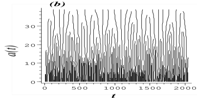
FIG. 1.: (a) – the path of a Brownian particle; (b) – the modulus-maxima skeleton of the random signal pictured in (a); (c) – the dependence $\tau(q)$; (d) – the singularity spectrum. The first derivative of the Gaussian function was used as the analyzing wavelet.

III multifractal approach to stochastic resonance

We treat for our study the overdamped bistable oscillator which is governed in canonical units [2] by the following stochastic differential equation (SDE):

$$\dot{x}=x-x^{3}+\sqrt{2Q}\,\xi(t)+y(t),$$ (3)

where $\xi(t)$ is the white Gaussian noise with the correlation function $\langle\xi(t)\>\xi(t^{\prime})\rangle\>=\>\delta(t-t^{\prime})$ and $\langle\xi(t)\rangle\>=\>0$, $y(t)$ is an input signal.

In the following subsections, we present the results of numerical simulations of Eq. (3) for different kinds of input signal. To characterize SR from the multifractal formalism point of view we will process the sequences of the return times to the one of the potential wells [2] normalized on a characteristic time scale of an external driving force.

A Periodic input signal

Let us start from the more simple and well studied case of periodic external driving when $y(t)=A\,\sin(\Omega t+\phi)$. The amplitude of the input signal is assumed to be small, i.e., the signal alone cannot switch the system from one state to another in the absence of noise. For the low-frequency periodic modulation considered in this paper this means

$$A\leq A_{0}=\frac{2}{3\sqrt{3}}.$$ (4)

As is well known, the study of SR can be conditionally separated on the two cases. The first one deals with the situation of a weak input signal when the amplitude of periodic driving is very small in comparison with a potential barrier and can be considered in the framework of the LRT [16, 15]. The second one is beyond the limits of LRT and corresponds to an amplitude of a subthreshold input signal comparable with a barrier. In the last case, the dynamics of a bistable system is characterized by a high degree of coherence between the switching process and input signal [27]. It can be correctly described in terms of the phase synchronization theory both for periodic [28], chaotic [29] and stochastic input signals [30]. Moreover, as was shown in [31] SR takes the form of the noise-induced order in this case. Such information-theoretical measures as the source entropy and the dynamical entropy display a minimum at an optimal noise intensity.

FIG. 2.: (a) $D(h)$ in the case of the weak periodic input signal $A\>=\>0.081,\Omega\>=\>0.004$ for different values of noise intensity $Q$; (b) $\tau(q)$ corresponding to the singularity spectrums, $D(h)$, in (a) for different values of noise intensity; the return time sequences normalized on the external force period and corresponding singularity spectrums in the case of $A\>=\>0.286,\Omega\>=\>0.004$ for $Q=0.040$ ((c) and (d)) and $Q=0.012$ ((e) and (f)). The Gaussian function was used as the analyzing wavelet.

In order to describe quantitatively these different situations from the multifractal formalism point of view, we calculated singularity spectrums for different values of the driving amplitude taking as the signal under study a sequence of the return times normalized on the driving period. Each sequence contained 10000 points. The results of calculations have shown the following. Singularity spectrum of the response has a bell shape form both in the presence and in the absence of the external periodic driving. That caused by a nonlinearity of the bistable system’s response to the external driving force which manifests itself in the presence of the different modes and in their interaction. As seen from Fig. 2, the tuning of noise level in the system of Eq. (3) leads to the changes in singularity spectrum both for weak and for strong enough driving signals. The width of the singularity spectrum takes its minimal value for an optimal noise intensity. It remains finite in the case of a weak periodic driving force, whereas in the regime of stochastic synchronization singularity spectrum qualitatively changes its form shrinking to a single point. The return times fluctuate around the driving period in the regime of noise-enhanced phase locking and large bursts are seldom happen (Fig. 2 $(c)$), while for the values of noise intensities lying outside of synchronization region the respectively large fluctuations dominate (Fig. 2 $(e)$).

FIG. 3.: The degree of multifractality, $\beta$, vs. noise intensity for different values of the periodic force amplitude: $A\>=\>0$ (stars), $A\>=\>0.081$ (triangles), $A\>=\>0.152$ (diamonds), $A\>=\>0.268$ (circles). The frequency of external force has the same value as in Fig. 2 The Gaussian function was used as the analyzing wavelet.

It is natural to consider the degree of multifractality $\beta$ defined as the difference between the maximal and minimal Hölder exponents belonging to the one and the same singularity spectrum as a new measure for SR and stochastic synchronization. As clearly seen from Fig. 3, the dependence of $\beta$ on the noise intensity is characterized by the presence of a minimum both for weak and for sufficiently strong input signals. In the regime of stochastic synchronization $\beta$ equals to zero that corresponds to a single point singularity spectrum (see Fig. 2 (d)). In this case the scaling features of the return time sequence under study is characterized by the single scaling exponent that caused by the linearization of the response in the regime of switchings synchronization. Indeed, the interaction between different modes in response is suppressed in synchronous regime, because the switchings in the system (3) are in-phase with the input signal. The mode corresponding to the periodic input signal dominates and suppresses all others.

FIG. 4.: Regions of stochastic synchronization constructed by means of effective diffusion constant (dashed line) and of multifractality degree (solid line). Driving frequency is $\Omega\>=\>0.004$. The Gaussian function was used as the analyzing wavelet.

In turn, it leads to simplification of the singularity spectrum that reflects the absence of interactions between Fourier phases in response. It is necessary to emphasize here, that we understand stochastic synchronization as instantaneous matching of the input/output phases which is observed in a finite region on the parameter plane “noise intensity – amplitude of periodic force”. Traditionally, synchronization in noisy nonlinear oscillatory systems is estimated quantitatively by means of effective diffusion constant which characterizes a velocity of spreading of an initial phase difference distribution [32]. Recently, this classical approach to synchronization was successfully used for quantitative description of the noise-enhanced phase coherence which takes place in stochastic bistable system driven by a subthreshold external signal [28, 29, 30]. The effective diffusion constant demonstrates a minimum decreasing up to a very small value in the region of synchronization. The above introduced wavelet-based measure demonstrates exactly the same behavior taking the zero value in the phase-locking regime that allows us to consider it as the measure of stochastic synchronization as well.

FIG. 5.: The degree of multifractality vs. noise intensity calculated for indicated values of the length of the return time sequence. The amplitude and frequency of the driving force are $A\>=\>0.12$, $\Omega\>=\>0.004$.

Using $\beta$ as the measure of stochastic synchronization it is possible to construct the region of synchronization on the parameter plane “noise intensity - amplitude of periodic force” (see Fig. 4). Inside of this region singularity spectrum of the response remains monofractal that once more time demonstrates the simplification of the response in the regime of synchronization. Synchronization region has a tongue-like form and nearly coincides with the similar one constructed by means of the effective diffusion constant used in [28, 29, 30]. It should be noted that the degree of multifractality does not relate directly with effective diffusion constant. The multifractal approach based on the analysis of the scaling features of the temporal sequence whereas the effective diffusion constant is the value characterizing a probability distribution of the input/output instantaneous phase difference. Our numerical studies also have shown that $\beta$ demonstrates a monotonous dependence on the driving frequency.

The length of the analyzed signals becomes the important parameter if they obtained in real experiments with live objects. Evidently, to estimate the possibility to use the above proposed measure in real situations we need to test its ability to catch SR for different lengths of the return time sequences. The results of our computations have been shown that the degree of multifractality takes the possibility to observe SR both for long and for sufficiently short return time sequences. As seen from Fig. 5, $\beta$ calculated over the short return time sequences containing only 1000 points demonstrates nearly the same behavior as in the case of the long sequences.

FIG. 6.: Spectral power amplification vs. noise intensity for different values of the driving amplitude. Driving frequency is $\Omega\>=\>0.004$.

Thus, the width of singularity spectrum manifests itself as the general and universal characteristic for description of SR, because it works very well in a wide range of values of the driving amplitude and frequency. Its calculation allows us to get the information about the scaling properties of the frequency fluctuations of a nonlinear system response and doesn’t requires any information about input signal. Moreover, that new characteristic allows one to analyze effectively a response even in the case of short return time sequences that has an especial meaning for possible applications.

The obtained results are in a good agreement with the behavior of the spectral power amplification $\eta$ firstly used for quantitative characterization of SR in [2, 7]. It demonstrates a maximum the absolute value of which is increased with the decrease of the input driving amplitude (see Fig. 6). The values of noise intensity maximizing $\eta$ nearly coincide with the ones minimizing the degree of multifractality. The growth of the driving amplitude leads to the shift of minimal values of $\beta$ to lower noise level as well as for spectral power amplification.

B Stochastic input signal

From the practical application point of view, it is more interesting the situation when an input signal has a complex structure. SR for the input signals with fluctuating amplitude and phase was considered in [33, 34]. In order to model the situation when the external signal is close to periodic one, but has a finite width of the spectral line Neiman and Schimansky-Geier [34] proposed to consider the harmonic noise as the input signal. Using the cumulant analysis and computer simulations they showed that the effect of SR takes place for harmonic noise as well and the width of the spectral line of the input signal at the output power spectrum can be decreased via SR.

Harmonic noise $y(t)$ is defined by the following two-dimensional SDE [33, 34]:

$$\dot{y}\>=\>s,\hskip 14.22636pt\dot{s}\>=\>-\Gamma s-\Omega^{2}y+\sqrt{2\varepsilon\Gamma}\>\zeta(t),$$ (5)

where $\zeta(t)$ is the zero-mean Gaussian noise with $\langle\zeta(t)\>\zeta(t^{\prime})\rangle\>=\>\delta(t-t^{\prime})$. It is necessary to note, that Gaussian noise $\zeta(t)$ is statistically independent from the noise $\xi(t)$ in (3). Equation (5) determines the two-dimensional Ornstein-Uhlenbek process $y(t),\>s(t)$ with the power spectrum

$$S_{yy}(\omega)\>=\>\frac{\Gamma\varepsilon}{\omega^{2}\>\Gamma^{2}+(\omega^{2}-\Omega^{2})^{2}},$$ (6)

which for $\Omega^{2}>\Gamma^{2}/4$ has a peak at the frequency $\omega_{p}\>=\>\sqrt{\Omega^{2}-\Gamma^{2}/2}$ with the width

$$\Delta\Omega\>=\>\sqrt{\omega_{p}^{2}+\Gamma\omega_{1}}-\sqrt{\omega_{p}^{2}-\Gamma\omega_{1}},$$ (7)

where $\omega_{1}\>=\>\sqrt{\Omega^{2}-\Gamma^{2}/4}$. The mean square displacements $\langle y^{2}\rangle=\varepsilon/\Omega^{2},\langle s^{2}\rangle=\varepsilon,\langle ys\rangle=0$. The increase of the parameter $\Gamma$ causes the widening of the spectral line [34]. We used harmonic noise as the input signal in (3) to carry out the multifractal analysis of SR in the case of aperiodic driving force. As in the previous subsection, we analyzed the return time sequences containing the same amount of points as before and normalized on the period $T=2\pi/\Omega$. To compare our results with those obtained previously, we choose the same values of parameters for numerical simulations as in [34]. The results of our computations are presented in Fig. 7. The difference between the maximal and minimal Hölder exponents takes its minimal value for an optimal noise intensity as in the case of periodic driving. The obtained results are in good agreement with the results of [34].

FIG. 7.: The degree of multifractality of the bistable system (3) response to the harmonic noise vs. noise intensity for the different values of the dissipation parameter in (5). Other parameters are $\Omega\>=\>0.1,\varepsilon\>=\>0.025$.

The degree of multifractality behaves as the relative width of the output spectral line used in [34] demonstrating the minimum at a close value of the noise intensity. The decrease of $\Gamma$ in (5) leads to the regularization of the input signal that makes the minimum in $\beta(D)$ more pronounced.

C Chaotic input signal

Now, let us take as the input signal in (3) the slowly varying subthreshold chaotic signal generated by the Lorenz system which is governed by the following ordinary differential equations:

$$\dot{y_{1}} = 10\>(y_{2}-y_{1})\nu,$$ (8)

$$\dot{y_{2}} = (28\>y_{1}-y_{2}-y_{1}y_{3})\nu,$$ (9)

$$\dot{y_{3}} = (y_{1}y_{2}-8/3\>y_{3})\nu,$$ (10)

where $\nu$ is the small rationing constant slowing chaotic oscillations. Lorenz attractor existing in the phase space of this system has a thin multifractal structure [35].

FIG. 8.: The input (a) and output (b) signals in the regime of stochastic synchronization for the case of chaotic driving signal generated by the Lorenz signal. The parameters are $k=0.0188$, $Q=0.03$, $\nu=0.005$.

FIG. 9.: Singularity spectrums for different values of noise intensity $Q$ and of the rationing constant: (a) $k=0.01$, (b) $k=0.0188$

FIG. 10.: The degree of multifractality vs. noise intensity for the different values of chaotic signal amplitude. The width of the singularity spectrum of the input signal is represented by the dashed line. The Gaussian function was used as the analyzing wavelet.

The power spectrum of chaotic oscillations calculated for $y_{1,2}$-variables does not contain any sharp peaks in this case. The input signal has a form of random process of switchings between two metastable states (see Fig. 8 $(a)$). It is reasonable to calculate the return time sequences for the input and output signals and then to try to estimate the distortion of the signal in stochastic resonator using singularity spectrum. We used the variable $k\cdot y_{1}(t)$ from the system of Eq. (8) as the input signal in our simulations, here $k$ is a small positive rationing constant. As follows from the results presented in Fig. 9 $(a)$, singularity spectrums of the input and output signals become more close to each other for some optimal noise level. Moreover, for some values of the parameter $k$ the noise-enhanced phase coherence between chaotic signal and response is observed [29]. In this case, the switchings in the input signal are in phase with the switchings in stochastic bistable system (see Fig. 8). Singularity spectrums of the input signal and of the response are coincide (see Fig. 9 $(b)$) in the regime of phase locking that means the passing of chaotic signal through the stochastic resonator without any distortions. This is also illustrated by the dependence of the singularity spectrum’s width on the noise intensity for bistable system response that is presented in Fig. 10. For some optimal noise intensity, $\beta$ takes its minimal value closing to the value corresponding to the width of the input signal’s singularity spectrum. As was mentioned above, the input and output singularity spectrums coincide in the regime of stochastic synchronization that causes the coincidence of $\beta$ with the multifractality degree of the external chaotic signal in some finite range of noise intensities.

IV multifractal analysis of neuron spike trains

One of the reason for unremitting interest in SR is the possibility to model on its base different cooperative effects and the process of the information transfer in various biological sensory systems operating in natural noisy environment. At present, there are a lot of experimental results showing that sensory neurons of different live organisms are able to demonstrate SR [36, 4]. In order to estimate the enhancement of a response, the signal-to-noise ratio or different cross-correlation measures are usually used [14, 36]. It is very interesting to use the above multifractal approach to analyze the spike trains generated by a stochastic neuronal model.

We took as a model the Fitzhugh-Nagumo system [37] operating in excitable regime and driven by a mixture of the internal noise and a subthreshold stochastic spike train generated by another similar system detuned from the first one on a control parameter. The unidirectionally coupled neuron systems are described by the following stochastic differential equations:

$$\mu\dot{x_{1}} = x_{1}-\frac{x_{1}^{3}}{3}-y_{1}$$ (11)

$$\dot{y_{1}} = x_{1}+a_{1}+k\,x_{2}+\sqrt{2\,Q_{1}}\>\xi_{1}(t)$$ (12)

$$\mu\dot{x_{2}} = x_{2}-\frac{x_{2}^{3}}{3}-y_{2}$$ (13)

$$\dot{y_{2}} = x_{2}+a_{2}+\sqrt{2\,Q_{2}}\>\xi_{2}(t)$$ (14)

where $a_{1}$ ($Q_{1}$) and $a_{2}$ ($Q_{2}$) are, respectively, the control parameters (noise intensities) of the subsystems $(x_{1},y_{1})$ and $(x_{2},y_{2})$, $\xi_{1}$ and $\xi_{2}$ are the statistically independent Gaussian white noise with the zero mean, $k$ is a small rationing constant as before and $\mu\ll 1$ is a small parameter allowing one to separate all motions in the fast and slow ones. The values of control parameters and noise intensities in subsystems are different and varied independently from each other. Thus, we can consider the system of Eq. (11) as a model of a single neuron embedded in a network and driven by both the internal noise and summed output of the neibouring neurons that can be modeled as a stochastic spike train. Interspike intervals (ISI) widely used in neuroscience as the typical neuron signals will play the role of signals under study in our consideration. The input stochastic spike train generated by the second neuron is characterized by a continuous singularity spectrum having a finite width as well as the chaotic input signal from the Lorenz system.

FIG. 11.: Degree of multifractality of the first neuron response in Eq. (11) vs internal noise intensity $Q_{1}$. Parameters: $\mu=0.01,\>a_{1}=1.05,\>a_{2}=1.07,\>Q_{2}=0.02,\>k=0.025$. The width of the input signal singularity spectrum is labeled by the dashed line. The Gaussian function was used as the analyzing wavelet.

The calculated widths of the singularity spectrum for the ISI generated by the first neuron are shown in Fig. 11. It can be seen that the dependence of $\beta$ on the internal noise intensity is characterized by two different minimums corresponding to two different effects taking place in the system (11) for small and large internal noise level, respectively. The first minimum appearing at the comparatively small noise intensity corresponds to the effect of aperiodic stochastic resonance when a weak internal noise enhances the response of the neuron model optimizing the transmission of the input signal. As clearly seen from Fig. 11, the width of singularity spectrum calculated on the first neuron ISI is very close to the input one for some optimal values of noise level. Further increase of noise intensity makes singularity spectrum of response more narrow that can be considered as a manifestation of stochastic resonance without input signal [38] called coherence resonance in [39]. Indeed, in the case of sufficiently large noise intensity neuron already cannot distinguish the structure of the noisy input signal. It operates as an oscillator whose time scale is controlled by noise. For some optimal value of the internal noise intensity $Q_{1}$ oscillations of the first neuron become close to the periodic one that is the essence of coherence resonance [39]. At the moment when coherence resonance is observed $\beta$ takes its second deeper minimum reflecting the noise-enhanced ordering of ISI.

V conclusions

We have studied the phenomenon of stochastic resonance in terms of the multifractal formalism revisited with wavelets [25]. We observed that for some optimal noise intensity the degree of multifractality of the response, defined as a width of the singularity spectrum, takes its minimal value. Moreover, the qualitative change of its structure takes place in the regime of stochastic synchronization. In the region of the noise-enhanced phase locking it shrinks to the single point with zero Hölder exponent. We have shown that the width of the singularity spectrum calculated over the return time sequence can be effectively used as the measure characterizing the response of a noisy nonlinear system in a wide range of the driving amplitudes and frequencies. As follows from our numerical results this measure can be successfully used both for periodic and aperiodic (stochastic or chaotic) driving signals. Moreover, it has allowed us to estimate the degree of coherence for the unidirectionally coupled stochastic neurons model operating in excitable regime. By using the introduced measure, we successfully diagnose both aperiodic stochastic resonance and coherence resonance which take place in the model under study for the small and large noise intensities, respectively.

The proposed approach has a number of benefits in comparison with the traditionally used measures such as SNR, SPA, residence time distributions, coherence function and others. These measures use the averaging procedure for their calculation that leads to the loss of information about nonlinear interaction between Fourier phases in response. This information is very important both for deeper understanding of the essence of SR and for more sensitive diagnostic of SR in full-scale experiments. The multifractal formalism based on wavelet calculations allows to study the temporal structure of the response. It catches all even weak non-stationarityies in a return times sequence under study that makes it a very powerful tool for diagnostic of SR and stochastic synchronization. The introduced measure demonstrates the behavior which in a very good agreement with the behavior of traditional quantitative characteristics of SR. It is universal in relation to the kind of the input signal and able to catch noise-induced effects even from very short time series. Later has the especial importance for the analysis of real signals.

The presented approach to the study of scaling features of motion in stochastic systems may be very fruitful also in the case of the Brownian motion in periodic potential under the action of random forces. It will be the task of our future investigations.

FIGURE CAPTIONS:

Fig. 1. (a) – the path of a Brownian particle; (b) – the modulus-maxima skeleton of the random signal pictured in (a); (c) – the dependence $\tau(q)$; (d) – the singularity spectrum. The first derivative of the Gaussian function was used as the analyzing wavelet.

Fig. 2. (a) $D(h)$ in the case of the weak periodic input signal $A\>=\>0.081,\Omega\>=\>0.004$ for different values of noise intensity $Q$; (b) $\tau(q)$ corresponding to the singularity spectrums, $D(h)$, in (a) for different values of noise intensity; the sequences of the return times normalized on the external force period and corresponding singularity spectrums in the case of $A\>=\>0.286,\Omega\>=\>0.004$ for $Q=0.040$ ((c) and (d)) and $Q=0.012$ ((e) and (f)); The Gaussian function was used as the analyzing wavelet.

Fig. 3. Degree of multifractality vs. noise intensity for different values of the periodic force amplitude: $A\>=\>0$ (stars), $A\>=\>0.081$ (triangles), $A\>=\>0.152$ (diamonds), $A\>=\>0.268$ (circles). The frequency of external force has the same value as in Fig. 2. The Gaussian function was used as the analyzing wavelet.

Fig. 4. Regions of stochastic synchronization constructed by means of effective diffusion constant (dashed line) and of multifractality degree (solid line). Driving frequency is $\Omega\>=\>0.004$. The Gaussian function was used as the analyzing wavelet.

Fig. 5. Degree of multifractality vs. noise intensity calculated for indicated values of the length of the return time sequence. The amplitude and frequency of the driving force are $A\>=\>0.12$, $\Omega\>=\>0.004$.

Fig. 6. Spectral power amplification vs. noise intensity for different values of the driving amplitude. Driving frequency is $\Omega\>=\>0.004$.

Fig. 7. Degree of multifractality of the bistable system (3) response to the harmonic noise vs. noise intensity for the different values of the dissipation parameter in (5). Other parameters are $\Omega\>=\>0.1,\varepsilon\>=\>0.025$.

Fig. 8. The input (a) and output (b) signals in the regime of stochastic synchronization for the case of chaotic driving signal generated by the Lorenz signal. The parameters are $k=0.0188$, $Q=0.03$, $\nu=0.005$.

Fig. 9. Singularity spectrums for different values of noise intensity $Q$ and of the rationing constant: (a) $k=0.01$, (b) $k=0.0188$. The Gaussian function was used as the analyzing wavelet.

Fig. 10. Degree of multifractality vs. noise intensity for the different values of chaotic signal amplitude. The width of the singularity spectrum of the input signal is represented by the dashed line. The Gaussian function was used as the analyzing wavelet.

Fig. 11. Degree of multifractality of the first neuron response in Eq. (11) vs internal noise intensity $Q_{1}$. Parameters: $\mu=0.01,\>a_{1}=1.05,\>a_{2}=1.07,\>Q_{2}=0.02,\>k=0.025$. The width of the input signal singularity spectrum is labeled by the dashed line. The Gaussian function was used as the analyzing wavelet.

REFERENCES

- [1] R. Benzi, A. Sutera and A. Vulpiani, J. Phys. A: Math. Gen. 14, L453 (1981); R. Benzi, G. Parisi, A. Sutera and A. Vulpiani, Tellus 34 10 (1982); C. Nicolis and G. Nicolis, Tellus 33, 225 (1981); C. Nicolis, Tellus 34, 1 (1982).
- [2] P. Jung, Phys. Rep. 234, 175 (1993).
- [3] L. Gammaitoni, P. Hänggi, P. Jung and F. Marchesoni, Rev. Mod. Phys. 70, 223 (1998).
- [4] V. S. Anishchenko, A. Neiman, F. Moss, and L. Schimansky-Geier, Usp. Fiz. Nauk 169, 7 (1999) [Sov. Phys. Usp. 42, 7 (1999)].
- [5] S. Fauve and F. Heslot, Phys. Lett. 97A, 5 (1983).
- [6] B.McNamara, K.Wiesenfeld, and R.Roy, Phys. Rev. Lett. 60, 2626 (1988).
- [7] P. Jung and P. Hänggi, Phys. Rev. A 44, 8032 (1991).
- [8] L. Gammaitoni, F. Marchesoni, E. Menichella-Saetta, and S. Santucci, Phys. Rev. Lett. 62, 349 (1989).
- [9] T. Zhou, F. Moss, and P. Jung, Phys. Rev. A 42, 3161 (1990).
- [10] L. Gammaitoni, F. Marchesoni,and S. Santucci, Phys. Rev. Lett. 74, 1052 (1995).
- [11] M. H. Choi, R. F. Fox, and P. Jung, Phys. Rev. E 57, 6335 (1998).
- [12] M. E. Inchiosa and A. R. Bulsara, Phys. Rev. E 53, R2021 (1996).
- [13] J. W. C. Robinson, D. E. Asraf, A. R. Bulsara, and M. E. Inchiosa, Phys. Rev. Lett. 81, 2850 (1998).
- [14] J. J. Collins, C. C. Chow, and T. T. Imhoff, Phys. Rev. E 52, R3321 (1995); J. J. Collins, C. C. Chow, A. C. Capela, and T. T. Imhoff, Phys. Rev. E 54, 5575 (1996); C. Heneghan, C. C. Chow, J. J. Collins, T. T. Imhoff, S. B. Lowen, and M. C. Teich, Phys. Rev. E 54, R2228 (1996).
- [15] A. Neiman, L. Schimansky-Geier, and F. Moss, Phys. Rev. E 56, R9 (1997).
- [16] M.I. Dykman, R. Mannella, P.V.E. McClintock, and N.G. Stocks, Phys. Rev. Lett. 65, 2606 (1990).
- [17] P. Ch. Ivanov, M. G. Rosenblum, C.-K. Peng, J. Mietus, S. Havlin, H. E. Stanley, and A. L. Goldberger, Nature (London), 383, 323 (1996).
- [18] P. Ch. Ivanov, L. A. N. Amaral, A. L. Goldberger, S. Havlin, M. G. Rosenblum, Z. Struzik, and H. E. Stanley, Nature (London), 399, 461 (1999).
- [19] T. C. Halsey, M. H. Jensen, L. P. Kadanoff, I. Procaccia, and B. I. Shraiman, Phys. Rev. A 33, 1141 (1986).
- [20] A. Arnéodo, G. Grasseau, and M. Holschneider, Phys. Rev. Lett. 61, 2281 (1988).
- [21] S. Mallat, and W. L. Hwang, IEEE Trans. Inf. Theory 38, 617 (1992).
- [22] J. F. Muzy, E. Bacry, A. Arnéodo, Phys. Rev. Lett. 67, 3515 (1991).
- [23] J. F. Muzy, E. Bacry, A. Arnéodo, Phys. Rev. E 47, 875 (1993).
- [24] E. Bacry, J. F. Muzy, A. Arnéodo, J. Stat. Phys. 70, 635 (1993).
- [25] J. F. Muzy, E. Bacry, A. Arnéodo, Int. J. Bifurcation Chaos Appl. Sci. Eng. 4, 245 (1994).
- [26] S. Mallat, A Wavelet Tour of Signaling Processing (Academic Press, San Diego, 1998).
- [27] B. Shulgin, A. Neiman, and V. Anishchenko, Phys. Rev. Lett. 75, 4157 (1995).
- [28] A. Neiman, A. Silchenko, V. Anishchenko, and L. Schimansky-Geier, Phys. Rev. E. 58, 7118 (1998); V. S. Anishchenko, A. B. Neiman, A. N. Silchenko, and I. A. Khovanov, Dynam.Stabil.Syst., 14, 211 (1999).
- [29] A. Silchenko, T. Kapitaniak, and V. Anishchenko, Phys. Rev. E. 59, 1593 (1999).
- [30] A. Neiman, L. Schimansky-Geier, F. Moss, B. Shulgin, and J. J. Collins, Phys. Rev. E. 60, 284 (1999).
- [31] A. Neiman, B. Shulgin, V. Anishchenko, W. Ebeling, L. Schimansky-Geier, and J. Freund, Phys. Rev. Lett. 76, 4299 (1996);
- [32] R. L. Stratonovich, Topics in the Theory of Random Noise, Vol.2 (Gordon and Breach, New York, 1967).
- [33] L. Schimansky-Geier and Ch. Zülicke, Z. Phys. B 79, 451 (1990).
- [34] A. Neiman and L. Schimansky-Geier, Phys. Rev. Lett. 72 2988 (1994).
- [35] Kjell Ottar Wiklund and John N. Elgin, Phys. Rev. E. 54, 1111 (1996).
- [36] J. K. Douglass, L. Wilkens, E. Pantazelou, and F. Moss, Nature(London) 365, 337 (1993); J. J. Collins, T. T. Imhoff, and P. Grigg. J. Neurophysiol. 76, 642 (1996); P. E. Greenwood, L. M. Ward, D. F. Russell, A. Neiman, and F. Moss, Phys. Rev. Lett. 84 4773 (2000).
- [37] M. C.Cross, and P. C. Hohenberg, Rev. Mod. Phys. 65, 851 (1993).
- [38] Hu Gang, T. Ditzinger, C. Z. Ning, and H. Haken, Phys. Rev. Lett. 71, 807 (1993).
- [39] A. S. Pikovsky, and J. Kurths, Phys. Rev. Lett. 78, 775 (1997).
-
[40]
LastWave software freely available at
http://wave.cmap.polytechnique.fr/soft/LastWave