Generic spectral properties of right triangle billiards

Abstract

This article presents a new method to calculate eigenvalues of right triangle billiards. Its efficiency is comparable to the boundary integral method and more recently developed variants. Its simplicity and explicitness however allow new insight into the statistical properties of the spectra. We analyse numerically the correlations in level sequences at high level numbers ($>10^{5}$) for several examples of right triangle billiards. We find that the strength of the correlations is closely related to the genus of the invariant surface of the classical billiard flow. Surprisingly, the genus plays and important rôle on the quantum level also. Based on this observation a mechanism is discussed, which may explain the particular quantum-classical correspondence in right triangle billiards. Though this class of systems is rather small, it contains examples for integrable, pseudo integrable, and non integrable (ergodic, mixing) dynamics, so that the results might be relevant in a more general context.

1 Introduction

Polygon billiards have been studied both classically and quantum mechanically for roughly twenty years now [1]. These systems are situated right on the borderline between integrability and chaos. They are usually divided into two classes: the rational polygon billiards where all vertex angles are rational multiples of $\pi$, and the irrational ones where at least one vertex angle is an irrational multiple of $\pi$.

In the first case, there exist two constants of motion, so that one would expect integrability. However, due to singularities in the billiard flow, the invariant surface of the flow is not necessarily a torus (with genus $g=1$), but may be of a more complicated topology ($1\leq g<\infty$). This produces a very complicated classical dynamics (see: [2, 3, 4] and references therein). The systems are called integrable if $g=1$ and pseudo integrable [1] otherwise.

In the second case (the irrational polygon billiards), there is no second constant of motion. These systems are typically ergodic [2] and probably weakly mixing [5, 6], though the Kolmogorov-Sinai entropy [7] is always zero.

Quantum and semiclassical calculations have been performed from the very beginning [1, 8, 9, 10], but only recently [11, 12] it became possible to calculate sufficiently large level sequences at sufficiently high energies, such that correlation properties could be analysed directly. There are fundamental open questions:

• Do the correlations in the spectra of polygon billiards eventually become stationary at sufficiently high energy?

• Are there families of polygon billiards with common statistical properties (universality)?

• What is the signature of classical pseudo integrability in the quantum spectrum (quantum-classical correspondence)?

On the one hand, there has been numerical evidence [12], that at very high energies the spectra of irrational triangle billiards are statistically similar to spectra taken from the Gaussian Orthogonal Ensemble (GOE). On the other hand, based on the numerical study of the spectra of several rational right triangle billiards, it was proposed that pseudo integrability implies so called “intermediate statistics” [11]. For the nearest neighbour distribution [13] this means: linear increase at small spacings (as in the GOE case) and exponential fall-off at large spacings (as for a random Poissonian sequence). Intermediate statistics has also been found in the context of disordered systems at the metal-insulator transition point [14, 15, 16], which might indicate some relationship between both classes of systems.

This paper is mainly concerned with question (iii). We consider the one-parameter family of right triangle billiards, labeled by the value of the smallest vertex angle $0<\alpha\leq\pi/4$. For this class, a secular equation is derived, which identifies the eigenvalues as zeros of the determinant of a particular matrix $K(E)$. Though the matrix is infinite, its elements are given explicitly by very simple expressions. This makes $K(E)$ an ideal point of departure for numerical and analytical studies.

The most obvious characteristic of rational polygon billiards is the genus $g$ of the invariant surface of the classical Hamiltonian flow (the irrational polygon billiards can be included, setting $g=\infty$). Hence we will investigate in detail the relation between $g$ and the correlations in the quantum spectra. In the numerical part, level sequences are calculated at absolute level numbers $>10^{5}$ for various examples of right triangle billiards. This provides valuable complementary information to recent results from Bogomolny et al. [11]. In the analytical part, the matrix $K(E)$ itself is considered. Though $K(E)$ is a pure quantum mechanical object, it is shown that $g$ and $\gamma$ (which is closely related to $g$) play a crucial rôle for iterated mappings of the form $\Psi(n)=K^{n}(E)\Psi(0)$. Based on this observation, a mechanism is proposed, which can explain the connection between the genus $g$ and the correlation properties of the quantum spectrum.

In section 2 a secular equation is derived for the calculation of the eigenvalues of right triangle billiards. It is used in section 3 to obtain and analyse the level spacing distributions for several right triangles. In section 4 we analyse the properties of the matrix $K(E)$ itself, and we discuss the rôles of the two classical parameters $g$ and $\gamma$ in this context. The conclusions are presented in section 5.

2 Secular equation

Our point of departure is the observation, that any right triangle can be obtained from cutting an appropriate rectangle along its diagonal. This is used to derive a secular equation of drastically reduced dimension for the eigenvalues of the right triangle billiard.

Let $H_{0}$ be the Hamiltonian for the rectangle billiard with sides $a$ and $b$. Fixing the length scale by: $a^{2}+b^{2}=\pi^{2}$, the angle $\alpha:\tan\alpha=b/a$ suffices to characterize the system completely. Choosing an arbitrary corner of the rectangle billiard as the origin of a Cartesian coordinate system, its eigenvalues and the corresponding eigenfunctions may be written as follows:

$$\varepsilon(n,m) =\frac{1}{2}\left(\frac{n^{2}}{\cos^{2}\alpha}+\frac{m^{2}}{\sin^{2}\alpha}\right)\;,\quad n,m\geq 1$$ (1)

$$\Phi_{nm}(x,y) =\frac{2}{\sqrt{ab}}\sin\!\!\left(\frac{\pi}{a}nx\right)\sin\!\!\left(\frac{\pi}{b}my\right)\;.$$ (2)

Consider the total Hamiltonian $H$:

$$H=H_{0}+\eta\;W\;,\quad W=\delta\!\!\left(\frac{x}{a}-\frac{y}{b}\right)\;,$$ (3)

where the potential $\eta W$ is used to cut the rectangle billiard into two congruent right triangle billiards (a similar cut potential, though in a different context, has been used in [17]). As $\eta$ increases from $0$ to $\infty$, the spectrum of $H$ changes from the spectrum of the rectangle billiard (1) to the doubly degenerated spectrum of the two triangle billiards. For any $\eta$, the Hamiltonian $H$ is invariant under point reflection, so that the matrix representation of $H$ in the eigenbasis of $H_{0}$ is block diagonal. One block is spanned by the odd basis states $\{\Phi_{nm}|\;n+m:{\rm odd}\}$ and the other by the even ones $\{\Phi_{nm}|\;n+m:{\rm even}\}$. Both blocks can be diagonalised independently, leading to the same sequence of eigenvalues, which causes the degeneracy mentioned above.

In what follows we will work in the odd basis only. Let $q=n+m$ and $p=n-m$, and order the states (2) with increasing $q$, and for equal $q$, with increasing $p$. Consider the subset of states with fixed $q$ and $p=-q+2,\ldots,q-2$ as one block. Then truncating the basis at a maximal $q$-value $q_{\mbox{\tiny max}}$, one obtains $M=(q_{\mbox{\tiny max}}-1)/2$ blocks with $q-1$ states in each block (note that $q$ and $p$ are odd). In total this gives $N=(q_{\mbox{\tiny max}}^{2}-1)/4$ basis states. In this reordered basis, the matrix elements of $W$ are given by:

$$\eqalign{W_{qp;q^{\prime}p^{\prime}}&=\int_{0}^{a}\rmd x\int_{0}^{b}\rmd y\;\Phi_{nm}(x,y)\Phi_{n^{\prime}m^{\prime}}(x,y)\;\delta\left(\frac{x}{a}-\frac{y}{b}\right)\\ &=\;\frac{1}{2}\{\delta(|p|-|p^{\prime}|)+\delta(q-|p^{\prime}|)+\delta(q^{\prime}-|p|)+\delta(q-q^{\prime})\}\;,}$$ (4)

where $n=(q+p)/2,\;m=(q-p)/2$ (and similarly for the primed indices). For given $q_{\mbox{\tiny max}}$ the truncated matrix $W^{(N)}$ has only two distinct eigenvalues: $0$ and $M+1$, and the eigenspace of the latter has dimension $M$ (in other words: rank$[W^{(N)}]=M$). All eigenvectors with eigenvalue $M+1$ can be calculated explicitly, and after proper normalization we collect them (as column vectors) in the rectangular matrix $V$:

$$V_{k;qp}=\frac{1}{\sqrt{M+1}}\left\{\begin{array}[]{ll}0&:n_{q}<k\\ \sqrt{\frac{k+1}{k}}&:n_{q}=k\\ \frac{1}{k(k+1)}&:n_{q}>k\;,\;n_{p}<k+1\\ -\sqrt{\frac{k}{k+1}}&:n_{q}>k\;,\;n_{p}=k+1\\ 0&:n_{q}>k\;,\;n_{p}>k+1\end{array}\right.\;,$$ (5)

where $k=1,\ldots,M$, $n_{q}=(q-1)/2$ and $n_{p}=(|p|+1)/2$. The truncated total Hamiltonian may now be written as follows:

$$H^{(N)}=H_{0}^{(N)}+\eta(M+1)\;VV^{T}\;.$$ (6)

Dividing the Schrödinger equation $(E-H^{(N)})\Psi=0$ by $E-H_{0}^{(N)}$, one arrives after a few algebraic manipulations at the desired secular equation. It determines the eigenvalues of $H^{(N)}$ as the zeros of the following determinant:

$$0=\det\left(1+\eta\tilde{K}^{(M)}(E)\right)\;,\qquad\tilde{K}^{(M)}(E)=(M+1)\;V^{T}\frac{1}{E-H_{0}^{(N)}}V\;.$$ (7)

Taking the limit $\eta\to\infty$, the unit matrix in the first equation of (7) can be neglected, and one gets:

$$\det\tilde{K}^{(M)}(E)=0\;.$$ (8)

The advantage of this equation, is the reduced dimension $M\ll N=M(M+1)$. Such a reduction is typical for a boundary integral method (see for example [18]). The matrix elements of $\tilde{K}^{(M)}$ are given by the following expression:

$$\tilde{K}_{ij}^{(M)}=(M+1)\sum_{q=1}^{q_{\mbox{\tiny max}}}\sum_{p=-q+2}^{q-2}\frac{V_{i,qp}\;V_{j,qp}}{E-\varepsilon\left(\frac{q+p}{2},\frac{q-p}{2}\right)}\;,\quad q,p:{\rm odd}\;.$$ (9)

Being only interested in the zero eigenvalues of $\tilde{K}^{(M)}(E)$, any (symmetric) similarity transformation $K^{(M)}=L^{T}\tilde{K}^{(M)}L$ may be applied. The following choice for $L$ simplifies the problem considerably:

$$L = {\rm diag}(1,\ldots,1/M)\,\left(\begin{array}[]{cccc}1&-1\\ &\ddots&\ddots\\ &&\ddots&-1\\ &&&1\end{array}\right)\,{\rm diag}\!\!\left(1,\ldots,\sqrt{M(M+1)}\right)\,.$$ (14)

(15)

The resulting matrix $K^{(M)}(E)$ is defined in the same way as $K(E)$ in the equations (16)-(18) below, but with the coefficients $D_{j}=\sum_{i=0}^{M}d_{ij}$. Only in the limit $M\to\infty$, the expression for $D_{j}$ simplifies to the formula (19), as can be shown using the partial fraction expansion of the cot function [19].

To summarize, the right triangle spectrum is calculated using the secular equation ${\rm det}[K(E)]=0$, where $K(E)$ is constructed as follows:

$$K(E)=K_{F}(E)+K_{D}(E)\;.$$ (16)

The matrix elements of $K_{F}$ are given by:

$$\eqalign{[K_{F}]_{ij}=d_{ij}-d_{i,j+1}-d_{i-1,j}+d_{i-1,j+1}\;,\\ d_{ij}=d_{ij}^{+}+d_{ij}^{-}\;,\qquad d_{ij}^{\pm}=\frac{1}{e-q^{2}-p^{2}\pm 2qp\cos 2\alpha}\;,}$$ (17)

where the scaled energy $e=E/(2\sin^{2}2\alpha)$ is used, and $q=2i+1$, and $p=2j-1$. Note, that $q^{2}+p^{2}\mp 2qp\,\cos(2\alpha)=2\sin^{2}(2\alpha)\;\varepsilon[(q\pm p)/2,(q\mp p)/2]$, thus $q$ and $p$ may still be regarded as auxiliary quantum numbers for the rectangle billiard $H_{0}$. The matrix $K_{D}$ is tridiagonal:

$$[K_{D}]_{jj}=D_{j}+D_{j+1}\;,\qquad[K_{D}]_{j,j+1}=[K_{D}]_{j+1,j}=-D_{j}\;,$$ (18)

with the coefficients $D_{j}$, given by

$$D_{j}=\frac{\pi\;\sin\pi\omega}{2\omega\left(\cos\pi\omega+\cos\pi p\cos 2\alpha\right)}\;,\qquad\omega=\sin 2\alpha\;\sqrt{2e-p^{2}}\;.$$ (19)

Even though $\omega$ becomes imaginary for large values of $p$, the affected functions: sin and cos convert into sinh and cosh, and finally the coefficient $D_{j}$ remains real. Its asymptotic behaviour for large $j$ is: $D_{j}\sim\pi/(2|\omega|)$.

This result is the basis for the analysis in section 3 and section 4. The infinite matrix $K(E)$, as defined in (16)-(19), completely determines the spectrum of any right triangle billiard as the set of zeros of its determinant. For numerical purposes $K(E)$ must be truncated (see below), but one may get important information also from an analysis of the infinite matrix $K(E)$ itself.

For numerical calculations (section 3), $K(E)$ is truncated, keeping only those elements $K_{ij}(E)$ for which $i,j\leq M$. For meaningful results, $M$ must be at least so large, that $p_{\mbox{\tiny max}}^{2}>2e,\;p_{\mbox{\tiny max}}=2M-1$ [see the definition of $p$ above equation (18)]. Experience shows, that for accurate results (error less than $1\%$ of the mean level spacing), one should increase the size of the matrix further by approximately 10%. The zeros of $\det[K(E)]$ are identified, calculating the smallest eigenvalue in magnitude as a function of $E$. Using a standard root bracketing algorithm [20] we find those points at which the smallest eigenvalue of $K(E)$ passes the zero axis. The eigenvalues of $K(E)$ are strictly decreasing functions of $E$, and this facilitates the root finding considerably. It allows to take rather large steps (of the order of the mean level distance), without running the risk to loose any roots.

3 Level spacing distributions

In the case of polygon billiards, the genus $g$ of the invariant surface of the Hamiltonian flow is the most obvious parameter to characterize the classical dynamics [2]. Hence one may expect an influence of $g$ on the level statistics of the corresponding quantum system. In this section we investigate numerically whether the level statistics show a systematic dependence on $g$. For several rational and one irrational right triangle, we calculate sequences of $10^{4}$ levels starting at the absolute level number $10^{5}$ (Weyl’s law is used to determine the corresponding energy). Note that even in this energy region the level statistics are usually not stationary. This has been demonstrated in [12] for several examples of rational and irrational triangle billiards. This should be kept in mind in the discussion of the numerical results.

In the case of right triangle billiards, there is another relevant parameter intimately related to $g$ (see A). This is $\gamma$, the smallest integer such that $2\alpha\,\gamma/\pi\in\mathbb{N}$ (in the irrational case, we set $\gamma=\infty$). It is shown in A, that $\gamma$ is the smallest number of rhombuses which must be glued together to form the invariant surface of the billiard flow. Moreover we find, that $g={\rm int}(\gamma/2)$. Hence $\gamma$ implies a finer classification of the right triangle billiards than $g$ does.

Table 1: All rational right triangle billiards with $g\leq 7$, referenced by their smallest vertex angle $\alpha/\pi=p/q$, and ordered with respect to $g$ and $\gamma$. The first two entries for $g=g_{a}=1$ are the only integrable cases. The shaded entries refer to those cases analysed in [11], and the gray-scale corresponds to the value of $g_{a}$ (introduced there) as indicated in the last column.

• 

Up to an irrelevant energy scale, all right triangles may be labeled and identified through their smallest vertex angle $0<\alpha\leq\pi/4$. For rational right triangles one may also use the pair of relatively prime integers $p/q=\alpha/\pi$. This is done in table 1, where all rational right triangles with $g\leq 7$ are arranged with increasing $\gamma$ in the vertical direction, and with increasing $\alpha$ in the horizontal direction. The parameter $g_{a}$ is taken from [11], where it is introduced as “arithmetical genus”. The entries under-laid with a gray shade have been analysed there. The gray-scale corresponds to different values of $g_{a}$, as indicated in the last column. Further below, we will compare our results with those of [11].

Figure 1: Difference $\Delta I\,(s)$ of the integrated level spacing distribution to the semi-Poisson case. $\Delta I\,(s)$ is plotted for various values of $\alpha$ as indicated in (a). The abbreviation “irr” refers to $\alpha=\pi(3-\sqrt{5})/4$. Whereas (b) shows the raw data, (a) shows the corresponding smoothed curves (details in the text). The GOE expectation ($N\to\infty$ limit) is plotted in (a) and (b) as a dotted line.

We analyse the level statistics by means of the nearest neighbour spacing distribution $P(s)$ (the spacings are normalized to unit mean). Recently the question has been raised, whether the rational right triangles show intermediate statistics (i.e. a linear increase at small $s$ and exponential fall-off at large $s$). A simple analytical example is the so called “semi-Poisson” distribution [11]:

$$P_{\mbox{\tiny SP}}(s)=4s\;\rme^{-2s}\;.$$ (20)

Here, $P_{\mbox{\tiny SP}}(s)$ is simply used as a conveniant reference to compare with. The following quantity is plotted in figure 1:

$$\Delta I\,(s)=\int_{0}^{s}\rmd s^{\prime}\;\left\{P_{\mbox{\tiny Num}}(s^{\prime})-P_{\mbox{\tiny SP}}(s^{\prime})\right\}\;.$$ (21)

The theoretical curves in the figures 1(a) and (b) show the result for an infinite GOE spectrum, where $P_{\mbox{\tiny Num}}(s^{\prime})$ is replaced by the corresponding level spacing distribution (taken from [21]). While figure 1(b) shows the raw numerical data curves for various right triangle billiards, figure 1(a) shows the corresponding smoothed curves, in order to allow the identification of all the cases shown. For the smoothing, “natural smoothing splines” have been used, as provided in [22].

Let us first focus on the cases: $p/q=1/8,1/5,1/12,1/7,3/16$ (which correspond to a successive increase of $\gamma$ from $4$ to $8$), and $\alpha/\pi=(3-\sqrt{5})/4$ (where $\gamma=\infty$). The $\Delta I$-curves for these cases are plotted in figure 1(a) with a solid line and dashed lines of different dash lengths. Together with the results for the GOE and the Poisson ensemble (uncorrelated random sequence), they roughly span a one-parameter family of curves $\Delta I_{\sigma}(s)$. The parameter $\sigma$ may be called “correlation strength” and it may be calibrated, requiring that $\sigma=0$ gives the Poisson result (its graph is plotted in figure 4), $\sigma=1$ the GOE result, and $\sigma=1/2$ the semi-Poisson result. Note, that $\Delta I_{\sigma}(s)$ is introduced solely to facilitate the discussion of our results, so that it is not necessary to be more specific.

The $\Delta I$-curve for the irrational right triangle billiard comes closest to the GOE result. However, it remains almost in the middle between the semi-Poisson case and the GOE case ($\sigma\gtrsim 3/4$). Then follow the cases $p/q=3/16,1/7$, and $1/12$, for which $\sigma$ decreases in approximately equal steps. The $\Delta I$-curve for $p/q=1/12$ is closest to the semi-Poisson result ($\sigma\approx 1/2$). The last two curves with $p/q=1/5$, and $1/8$ tend slightly towards the Poisson result. They are so close to each other, that we would assign the same correlation strength to both of them ($\sigma\lesssim 1/2$). In all we may say, that the correlation strength $\sigma$ increases with increasing $\gamma$.

Finally we included two more cases: $p/q=1/10$ and $3/14$. In figure 1(a) the respective $\Delta I$-curves are plotted with dotted lines. Thus we can compare the $\Delta I$-curves for the $1/5$- and the $1/10$-triangle ($\gamma=5$), and the $\Delta I$-curves for the $1/7$- and the $3/14$-triangle ($\gamma=7$). Both cases show, that even for right triangles with the same value for $\gamma$, the respective $\Delta I$-curves may differ considerably. The relation between $\gamma$ and the correlation strength is apparently not very strict (at least not in the energy range considered).

In order to check, that our conclusions do not depend on the particular choice of the correlation measure, we repeated the analysis above, using the number variance $\Sigma^{2}(l)$ [13] instead of $\Delta I(s)$. The results were perfectly compatible, so that a more detailed discussion is omitted.

In the numerical analysis presented here, we concentrate on right triangle billiards with small values for $g$ and $\gamma$. The main reason is, that there is certainly an energy scale below which the quantum system cannot possibly “recognize”, whether the two hypotenuse angles $\alpha$ and $\beta$ are rational or not. Without any knowledge about this scale, small $g$ triangles are probably the more reliable examples, for the study of quantum signatures of pseudo integrability. Hence the triangles for which we can compare our results with those of [11] are only a few: $p/q=1/8,1/5,1/12$, and $1/7$.

The results obtained in [11] agree with those presented here, only up to a certain qualitative level. Beyond, we find that the correlation strength has decreased considerably in almost all cases. This may be due to the higher energy region considered here, which results in the rationality of the hypotenuse angles being more important. However, the $\Delta I$-curves of the first group of right triangles (with $4\leq\gamma\leq 6$) changed much less then the others, such that the separation between both groups has decreased. It seems that this separation was decisive for the introduction of the arithmetical genus $g_{a}$. The fact that this separation has become much smaller now, indicates that $g_{a}$ is probably not an appropriate alternative for $g$.

According to the numerical results presented in this section, it is possible to order the right triangle billiards with respect to the strength of the correlations found in their spectra, which coincides with that of increasing $\gamma$. This finding confirms the general conjecture, that the genus of the invariant surface of the classical billiard flow determines the strength of the spectral correlations on the quantum level. Though the spectral correlations are apparently not stationary at currently accessible energies, the ordering seems to be energy independent, as long as the level sequences to be compared, start with the same absolute level number.

4 The elliptic map

In the first part of this section it is shown, that the parameters $g$ and $\gamma$ (see A) associated with the classical dynamics of right triangle billiards, are important characteristics of the matrix $K(E)$ itself. On the one hand this may be surprising, because $K(E)$ arose from a pure quantum mechanical approach (see section 2), but on the other hand it is a strong indication for the importance of classical pseudo integrability on the quantum level. In the second part, we present a tentative explanation for the dependence of the spectral statistics on $g$ and $\gamma$.

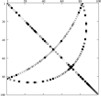
Figure 2: Portrait of the matrix $K(E)$ for $\alpha=\pi/5$, and $E=1.26\times 10^{4}$. The gray-scale corresponds to the absolute value of the matrix elements.

In figure 2 the matrix $K(E)$ is portrayed for a typical case. The gray-scale corresponds to the absolute value of the matrix elements. It can be seen, that most of the matrix elements have vanishingly small absolute values. Large absolute values can be found only along the diagonal and the first off-diagonals, which are due to $K_{D}$, and on a “moon”-like structure due to $K_{F}$ [see equations (17)-(19)]. The matrix elements $[K_{F}]_{ij}$ become large, whenever the pair of integers $(i,j)$ is close to the zero-line of one of the two functions

$$f_{\pm}(x,y)=e-4\left(x^{2}+y^{2}\pm 2xy\cos 2\alpha\right)\;,$$ (22)

where $x,y$ are real, and positive, and $e$ is the scaled energy as used in equation (17).

Figure 3: Schematic representation of the mapping $\vec{y}_{1}=K(E)\vec{y}_{0}$ (details see text).

The action of $K(E)$ on a localized state may be described schematically by a double valued, symmetric map as shown in figure 3. The square in the middle represents the matrix $K(E)$ (cf. figure 2). An initial state $\vec{y}_{0}$ localized at a given value $a_{0}$ is mapped to $\vec{y}_{1}=K(E)\vec{y}_{0}$ localized at $\{a_{0},a_{-1},a_{1}\}$, where $a_{-1}$ and $a_{1}$ are the two solutions of the equation $f_{\pm}(a_{0},x)=0$, for $x>0$. Hence, the map $M$ associated with $K(E)$ may be defined as follows: $\{a_{-1},a_{1}\}=Ma_{0}$. Let us call it the “elliptic map”. Due to $f(x,y)=f(y,x)$, $a_{0}\in Ma_{-1}$ and $a_{0}\in Ma_{1}$. Consequently, an orbit of such a map may be viewed as a doubly connected chain:

$$\cdots\!\!\!\parbox{210.55022pt}{\begin{picture}(0.0,0.0)\psfig{}\end{picture}\begin{picture}(12958.0,1368.0)(639.0,-2395.0)\put(7651.0,-1711.0){\makebox(0.0,0.0)[b]{\smash{$a_{0}$}}} \put(11251.0,-1711.0){\makebox(0.0,0.0)[b]{\smash{$a_{2}$}}} \put(13051.0,-1711.0){\makebox(0.0,0.0)[b]{\smash{$a_{3}$}}} \put(5701.0,-1711.0){\makebox(0.0,0.0)[b]{\smash{$a_{-1}$}}} \put(3601.0,-1711.0){\makebox(0.0,0.0)[b]{\smash{$a_{-2}$}}} \put(1501.0,-1711.0){\makebox(0.0,0.0)[b]{\smash{$a_{-3}$}}} \put(9451.0,-1711.0){\makebox(0.0,0.0)[b]{\smash{$a_{1}$}}} \end{picture} }\;\cdots$$ (23)

According to that picture, the $n$-fold image $\vec{y}_{n}=K(E)^{n}\;\vec{y}_{0}$ has localization peaks at the positions $\{a_{-n},\ldots,a_{0},\ldots,a_{n}\}$. Surprisingly, $M$ is isomorphic to the following, extremely simple map:

$$\varphi_{n\pm 1}=\varphi_{n}\pm 2\alpha\;,$$ (24)

where the result should be taken modulo $\pi$, such that it remains in the interval $\left[\right.-\pi/2,\pi/2\left.\right)$. This can be seen, using the following parametrisation of the curve $f_{\pm}(x,y)=0$:

$${x\choose y}=\sqrt{E}{\;\mbox{sgn}\left(\frac{\pi}{2}-2\alpha+\varphi\right)\;\cos(\varphi-2\alpha)\choose\cos(\varphi)}\;,\quad\varphi\in\left[\right.-\pi/2,\pi/2\left.\right)\;.$$ (25)

Replacing $y$ by an arbitrary point $a_{n}$ of the map $M$, one gets the corresponding pair conjugated angles: $\cos(\pm\varphi_{n})=a_{n}$. Replacing $x$ by $a_{n}$ one finds that $\pm\varphi_{n}$ must be mapped to $\pm\varphi_{n}-2\alpha$ (mod $\pi$). It follows, that

$$a_{n} = \cos(\pm\varphi_{n})$$

$$Ma_{n} = \{a_{n-1},a_{n+1}\}=\{\cos[\pm(\varphi_{n}-2\alpha)],\cos[\pm(\varphi_{n}+2\alpha)]\}\;.$$ (26)

From equation (24) it follows that any orbit is restricted to a set of $\gamma$ points, where $\gamma$ is the smallest integer such that $2\alpha\,\gamma/\pi\in\mathbb{N}$. It is the same $\gamma$, which is introduced in A as the number of rhombuses forming the invariant surface of the billiard flow. Furthermore, the periodicity of the map $M$ is ${\rm int}(\gamma/2)$ which is just the genus of that invariant surface.

Here in the second part of this section we discuss a mechanism which can explain the correspondence between the correlation properties of the quantum spectrum and the classical parameter $\gamma$. The line of reasoning is as follows:

• The correlation properties of the triangle spectrum at a given energy $E$ are closely related to the correlation properties of the eigenvalues of $K(E)$ in the vicinity of zero.

• At sufficiently high energy, $K_{D}$ (16) can be considered as a random tridiagonal matrix with eigenstates which are typically localized.

• The matrix $K_{F}$ (16) has such a form, that repeated multiplications of an initially localized state with $K(E)$, produce an increasing number of copies at different positions. The positions are given by the elliptic map $M$.

• If $\alpha$ is rational, all orbits of the elliptic map are periodic with period $g$ and restricted to $\gamma$ points. This leads to an approximate foliation of the Hilbert space into weakly coupled subspaces. For any irrational $\alpha$, the elliptic map is ergodic, and all basis states of the matrix $K(E)$ are strongly coupled.

Point 3 has been treated in the first part of this section. The remaining statements are discussed below.

Figure 4: Difference of the integrated level spacing distribution to the semi-Poisson case. In (a) $\Delta I\,(s)$ is plotted for the rational right triangle billiard with $\alpha/\pi=1/8$, in (b) for the irrational one with $\alpha/\pi=(3-\sqrt{5})/4$. The solid lines show the result for neighbored eigenvalues of the matrix $K(E)$, the dotted lines show the result for the triangle spectrum. The dashed lines show the theoretical curves for the Poisson case (long dashed lines) and for the GOE case (short dashed lines).

Correlation properties of the eigenvalues of the matrix $K(E)$

According to the secular equation derived in section 2, the triangle eigenvalues are given by those energies, at which at least one eigenvalue of $K(E)$ becomes zero. Therefore it seems plausible, that the correlation properties of the eigenvalues of $K(E)$ close to zero and the triangle eigenvalues are related. To verify this we calculate the spacing distribution for those two neighbouring eigenvalues which have opposite signs (without unfolding). The distribution is obtained from $10^{4}$ spacings, taken at equi-distant energies, with the step size adjusted to the mean level spacing of the corresponding triangle spectrum.

In figure 4 we compare the results. In the rational case (a) as well as in the irrational case (b), the $\Delta I(s)$-curves for the eigenvalue pairs of $K(E)$ and for the triangle spectra differ remarkably, though in (b) the agreement is somewhat better. However, at least qualitatively, the results are as expected: In the rational case, figure 4(a), the eigenvalue statistics for $K(E)$ show indeed very weak correlations, much weaker even than the corresponding triangle spectrum. This can be seen from the $\Delta I(s)$-curve which clearly tends towards the Poisson result (note also the behaviour at large $s$). In the irrational case, figure 4(b), both curves show relatively strong correlations.

Figure 5: The eigenstates of $K_{D}(E)$ with eigenvalues close to zero for a typical case. On the left, the absolute value of the eigenvector coefficients, plotted as a function of $i$, the index for the basis of $K(E)$. On the right, the corresponding eigenvalues plotted in a bar graph. $\alpha=\pi/5,E=1.5\times 10^{5}$.

Localization of the eigenstates of $K_{D}$

The matrix $K_{D}$ is constructed in a simple manner from the coefficients $D_{j}$ [see equations (18) and (19)]. Those oscillate as functions of $j$, the index of the basis of $K(E)$, more and more rapidly while $p^{2}$ approaches $2e$. From a statistical point of view, it then seems permissible to replace the arguments of the functions: sin and cos by appropriate random variables. Even though the statistical properties of the matrix elements are very complicated, one may expect Anderson localization [23].

In figure 5 we show for a typical case, a series of eigenstates of $K_{D}(E)$ ordered by their respective eigenvalues. Only those states with eigenvalues in a small interval around zero are shown. Many eigenstates are apparently localized. However, others are not, and spread over a wide range of basis states. Usually those fluctuate only weakly and slowly and their eigenvalues decrease very slowly with energy (not shown). Their rôle is still unclear, and will be the subject of future studies.

Foliation of the Hilbert space

Acting repeatedly with $K(E)$ on an initially localized state $\vec{y}_{0}$, the first $g$ images will spread and localize at points $\{a_{0},\ldots,a_{\gamma-1}\}$ (here $a_{\gamma-1}$ is identical to $a_{-1}$), as discussed in the first part of this section. Then, due to the periodicity of the elliptic map, subsequent images spread only slowly away from these points. In the ideal case the spreading would stop due to Anderson localization, giving rise to an invariant subspace. In the same way, an initial state localized in a different part of the Hilbert space, would lead to another invariant subspace, and so on – until possibly the whole Hilbert space would have been decomposed into invariant subspaces. In the real system, such a foliation of the Hilbert space occurs only approximately, and the subspaces become weakly coupled. Nevertheless one may expect, that correlations are to some extent suppressed due to this mechanism.

For irrational $\alpha$, where the elliptic map is ergodic, an initially localized state will spread out [by repeated multiplication with $K(E)$] into the whole Hilbert space. No foliation of the Hilbert space can occur, and one should expect correlations of similar strength as in the GOE case.

5 Conclusions

We derived a new kind of secular equation for the determination of the spectra of right triangle billiards. It involves the diagonalisation of the matrix $K(E)$ which has a particularly simple and transparent structure. Based on this equation we calculated spectra at level numbers $>10^{5}$ for various examples of right triangle billiards, which shows the efficiency of the new method.

We found a clear correspondence between the genus $g$ (or the related parameter $\gamma$) of the invariant surface of the classical billiard flow and the strength of the correlations in the quantum spectrum. While for small $g$ the spectral statistics is close to semi-Poisson (with a slight tendency towards Poisson), it approaches the GOE statistics when $g$ is increased. Our numerical results together with similar studies [11, 12] suggest that the spectral correlations are not stationary at currently accessible energies, but that the ordering with increasing correlation strength and its correspondence to $g$ is conserved.

In the second part of the paper, we found that the classical parameters $g$ and $\gamma$ are characteristic quantities for the matrix $K(E)$ itself. For rational right triangle billiards, where $g$ is finite, one gets an approximate foliation of the Hilbert space into invariant subspaces. The size of the subspaces scales with $\gamma$. Based on this observation, we discussed a mechanism which can explain the influence of $g$ and $\gamma$ on the level statistics of right triangle billiards.

The definition of $\gamma$ in A can be generalized to arbitrary polygon billiards as follows: $\gamma$ is the smallest number of identical polygons which must be glued together to form the invariant surface of the billiard flow. In this general case, $g$ and $\gamma$ must possibly be considered as independent parameters. Which of them is then more relevant for the correlations in the quantum spectrum? Considering the rôles of $g$ and $\gamma$ in the description of the matrix $K(E)$, it seems that this is $\gamma$ (the size of the approximate invariant subspaces of $K(E)$ scales with $\gamma$).

Appendix A The invariant surface for the classical billiard flow

There is an elegant way to represent a trajectory moving in a polygon billiard, which is particularly useful to construct the invariant surface of the classical billiard flow. It consists in drawing the trajectory as a straight line, and reflecting the billiard (instead of the trajectory) each time the boundary is hit [2]. In the case of rational polygons all possible trajectories can produce only a finite number of differently oriented copies of the original polygon. Then there is a general recipe of how to glue these copies together, in order to obtain the invariant surface.

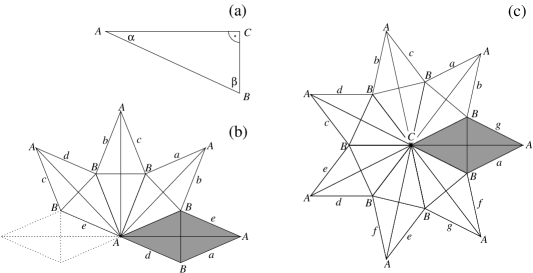
Figure 6: (a) Typical right triangle. (b) Invariant surface of the billiard flow for the $1/8$-triangle. The dotted rhombus does not form part of the invariant surface. (c) Invariant surface of the billiard flow for the $1/7$-triangle. In (b) and (c): the initial rhombuses, with which the rosette constructions are started are filled. Vertices are labeled by capital letters, edges by lower case letters. However, only such edges or vertices are labeled, which must be identified with one another, to obtain the invariant surface.

For rational right triangles one may follow a more explicit construction scheme, which leads to a particularly simple invariant surface; the “rosette”. It is constructed as follows: Start with a right triangle as depicted in figure 6(a). Reflecting the triangle on the side $AC$, the image on the side $BC$ and that image again on the side $AC$, produces a rhombus [see figure 6(b) and (c)]. This rhombus is rotated around point $A$ by the angle $2\alpha$ (counter-clockwise) at each step. Stop one step before arriving at the original rhombus or its point reflected image [see figure 6(b)]. Note, that the resulting surface may wind several times around $A$. As it is shown below, the resulting surface can be closed by identifying open edges with one another, which gives the invariant surface.

The number of rotations by $2\alpha$ is just the smallest integer $\gamma$ such that $2\alpha\,\gamma/\pi\in\mathbb{N}$. We could equally well rotate the rhombus step-wise by $2\beta$ around point $B$ [see figure 6(b) and (c)], resulting in a different representation of the invariant surface. However, as shown below, the number of rotations (or rhombuses) necessary to close the invariant surface is the same.

Proof: Let $p/q=\alpha/\pi$ and $p^{\prime}/q^{\prime}=\beta/\pi$ with $p,q$ and $p^{\prime},q^{\prime}$ relatively prime.

$$\eqalign{2\gamma\;\frac{p}{q}=l=2\gamma\left(\frac{1}{2}-\frac{p^{\prime}}{q^{\prime}}\right)&\Rightarrow\;2\gamma\;\frac{p^{\prime}}{q^{\prime}}=\gamma-l\;,\\ 2\gamma^{\prime}\;\frac{p^{\prime}}{q^{\prime}}=l^{\prime}=2\gamma^{\prime}\left(\frac{1}{2}-\frac{p}{q}\right)&\Rightarrow\;2\gamma^{\prime}\;\frac{p}{q}=\gamma^{\prime}-l^{\prime}\;.}$$ (27)

Consider the first line of (27). As $2p<q$ it follows $\gamma-l>0$. But $\gamma^{\prime}$ is the smallest integer such that $2\gamma^{\prime}\;p^{\prime}/q^{\prime}\in\mathbb{N}$, hence: $\gamma^{\prime}\leq\gamma$. The same argument applied to the second line of (27) shows: $\gamma\leq\gamma^{\prime}$. Therefore: $\gamma=\gamma^{\prime}$.

It remains, to prove that the procedure above gives indeed a representation of the invariant surface, and to calculate its genus $g$. To this end we show that all free edges of the rosette can be identified with one another. Then the rhombuses define a triangularisation of the invariant surface, and counting all faces $F$, edges $E$ and vertices $V$ of the triangularisation, we obtain the genus via the Euler characteristic [2]: $g=1-\chi/2,\chi=V-E+F$.

The edges may be divided into inner edges, which are connected to the center of the rosette, and outer edges, which are not connected to the center. Let us label both groups counter-clockwise by e₁,…and e${}_{1}^{\prime}$,…respectively, beginning with the lower edges of the initial rhombus (see figure 6, but note that the labels shown there are different, and used only to identify different edges in the representation of the invariant surface).

Let us first discuss the case, where $q$ is odd. Then $\gamma=q$ and the rosette winds $p$ times around its center before the last inner edge can be identified with the first one [see figure 6(c)]. In order to identify all outer edges e₁,…,e_2γ pairwise with one another, observe that for $j$ :odd, a trajectory leaving the surface crossing e_j+3 would enter a triangle which is the parallel translation of the triangle with the hypotenuse e_j. By consequence, both edges can be identified. Hence one may identify the following edges: e${}_{1}\equiv$ e₄, e${}_{3}\equiv$ e₆, …, e${}_{2\gamma-3}\equiv$ e_2γ, and there are only two open outer edges left: e₂ and e_2γ-1 which can be identified with one another on the same grounds.

The vertices in the representation of the invariant surface have to be identified taking into account that edges identified previously have the same initial and end points (the triangle connected to the edge defines an orientation). In this manner it is shown that for $q$ :odd, the rosette (invariant surface) has $\gamma$ faces, $2\gamma$ edges and $3$ vertices. Hence $\chi=3-\gamma$ and $g=(\gamma-1)/2$.

If $q$ is even, then $p$ (relatively prime) is odd and the rosette winds $p/2$ times around its center [see figure 6(b)] which means, that we have also two open inner edges: e${}_{1}^{\prime}$ and e${}_{\gamma+1}^{\prime}$. Identifying outer edges as explained above, leaves two outer edges open: e₂ and e_2γ-1. In this case we identify e${}_{1}^{\prime}$ with e_2γ-1 and e₂ with e${}_{\gamma+1}^{\prime}$, which again closes the invariant surface. Note that due to the identification of outer edges with inner edges, the central point of the rosette must be identified with the outermost points. The remaining points, must be identified as one single vertex $B$, if $\gamma$ is even [see figure 6(b)], otherwise they constitute two vertices $B$ and $B^{\prime}$ (this case is not shown). Hence the rosette (invariant surface) has $\gamma$ faces, $2\gamma$ edges, and $2$ vertices if $\gamma$ is even and $3$ vertices if $\gamma$ is odd. This gives $\chi=2-\gamma\Rightarrow g=\gamma/2$ and $\chi=3-\gamma\Rightarrow g=(\gamma-1)/2$ respectively.

In all: $g=(\gamma-1)/2$ if $\gamma$ :odd, and $g=\gamma/2$ if $\gamma$ :even. Hence $g={\rm int}(\gamma/2)$.

References

References

- [1] Richens P J and Berry M V 1981 Physica 2D 495–512
- [2] Gutkin E 1986 Physica 19D 311–33
- [3] Gutkin E 1996 J. Stat. Phys. 83 7
- [4] Kenyon R and Smillie J 2000 Comment. Math. Helv. 75, 65–108
- [5] Artuso R, Casati G and Guarneri I 1997 Phys. Rev. E 55 6384–90
- [6] Casati G and Prosen T 1999 Phys. Rev. Lett. 23 4729–32
- [7] Lichtenberg A J and Liebermann M A 1983 Regular and stochastic motion (New York: Springer)
- [8] Gaudin M 1987 J. Physique 48 1633–50
- [9] Shudo A and Shimizu Y 1993 Phys. Rev. E 47 54–62
- [10] Miltenberg A G and Ruijgrok T W 1994 Physisca 210A 476–88
- [11] Bogomolny E B, Gerland U and Schmit C 1999 Phys. Rev. E 59 R1315–18
- [12] G. Casati and T. Prosen. private Communication/Preprint, (1999).
- [13] Bohigas O 1991 Proc. Summer School on Theoretical Physics (Les Houches) session LII (Amsterdam: North Holland) p 86–199
- [14] Shklovskii B I, Shapiro B, Sears B R, Lambrianides P and Shore H B 1993 Phys. Rev. B 47 11487–90
- [15] Braun D, Montambaux G and Pascaud M 1998 Phys. Rev. Lett. 81 1062–65
- [16] Varga I and Braun D 2000 Phys. Rev. B 61 R11859–62
- [17] Lewenkopf C H 1990 Phys. Rev. A 42 2431–33
- [18] Vergini E and Saraceno M 1995 Phys. Rev. E 52 2204–07
- [19] Abramowitz M and Stegun I A 1964 Handbook of mathematical functions (New York: Dover)
- [20] Press W H 1992 Numerical recipes in Fortran (Cambridge: University Press)
- [21] Haake F 1991 Quantum signatures of chaos (Berlin: Springer Verlag)
- [22] 1999 Gnuplot Linux version 3.7 patchlevel 1
- [23] Anderson P W 1958 Phys. Rev. 109 1492