Classical invariants and the quantum-classical link

Abstract

The classical invariants of a Hamiltonian system are expected to be derivable from the respective quantum spectrum. In fact, semiclassical expressions relate periodic orbits with eigenfunctions and eigenenergies of classical chaotic systems. Based on trace formulae, we construct smooth functions highly localized in the neighborhood of periodic orbits using only quantum information. Those functions show how classical hyperbolic structures emerge from quantum mechanics in chaotic systems. Finally, we discuss the proper quantum-classical link.

For more than 20 years a lot of effort has been done in order to clarify the interplay between quantum and classical behavior in chaotic systems. Periodic orbit theory shows the important role that classical invariants play in quantum mechanics. For example, the Gutzwiller trace formula relates the quantum spectral density with classical periodic orbits [1].

Less is known about the interplay between the neighborhood of periodic orbits (the stable and unstable manifolds) and quantum mechanics. The first step was given by Bogomolny [2] who found the semiclassical contribution of periodic orbits and their vicinities to wave functions smoothed in energy and position. Advances in this issue contribute, among others, to the study of the morphologies of wave functions of chaotic systems. Especially, this gives new insights to the debated problem, the scarring phenomena [3], an anomalous localization of quantum probability density along unstable periodic orbits in classically chaotic systems. For example, Kaplan and Heller [4] proposed test states constructed by coherent wave-packet sums centered on a periodic orbit. The constructed wave function lives not only on the periodic orbit, but also along the linearized invariant manifolds. On the other hand, Vergini and Carlo [5, 6] developed a semiclassical construction of wave functions on periodic orbits and their neighborhoods (the stable and unstable manifolds) which are highly localized in energy. To resemble the classical hyperbolic structure, these constructions use the orbit and the linearized dynamics around it. The question that naturally arises is if the classical hyperbolic structure is present in quantum mechanics. An important contribution in this direction was given by Nonnenmacher and Voros [7]. They studied the eigenstates structures around a hyperbolic point in a one dimensional system.

In this letter, we address that question by constructing smoothed functions living on the periodic orbit and their manifolds and we use only the quantum information (the eigenvalues and eigenfunctions) of the system . This clearly will show the skeleton on which the quantum mechanics is built. Moreover, some features of these smoothed functions confirm predictions by Bogomolny and are well understood with the semiclassical construction of Ref. [5].

Our starting point is the Gutzwiller trace formula [1]. This formula evaluates the quantal spectrum of energy of a bounded system in terms of the classical spectrum of periodic orbits. We are going to consider billiard systems where the classical motion is described by straight lines between consecutive bounces with the boundary. The incoming and outgoing trajectories at a bounce satisfy specular reflection. A periodic orbit $\delta$ is characterized by the length $L_{\delta}$, and the Maslov index $\nu_{\delta}$. The quantum mechanics is given by the set of eigen-wavenumbers ${k_{n}}$ and eigenfunctions ${\phi_{n}(\vec{r})}$ which are defined by the Helmholtz equation $\;(\nabla^{2}+k_{n}^{2})\phi_{n}(\vec{r})=0\;$, with Dirichlet boundary conditions. For these systems, the trace formula reads [8]

$$\sum_{n}\delta(k-k_{n})=\rho(k)+\frac{1}{2\pi}\sum_{\delta}A_{\delta}\;e^{-ikL_{\delta}},$$ (1)

with

$$A_{\delta}=\frac{L_{\delta}\;e^{i\nu_{\delta}\pi/2}}{\sqrt{|\det(M_{\delta}-I)|}}.$$ (2)

and $M_{\delta}$ is the monodromy matrix of the orbit $\delta$. $\rho(k)$ is the mean level density

The Fourier transform of Eq. (1) gives the classical spectrum in terms of the quantal one [9]

$$f(L)\equiv\sum_{k_{n}<k}e^{ik_{n}L}-\tilde{\rho}(L)=\sum_{\delta}\frac{A_{\delta}\;\sin[k(L-L_{\delta})]}{2\pi\;(L-L_{\delta})}.$$ (3)

In particular, $\;f(L_{\delta})\simeq k\;A_{\delta}/2\pi\;$ and $|f(L)|^{2}$ has peaks at the length of the periodic orbits. Fig.  1 shows $|f(L)|^{2}$ obtained from the eigen-wavenumbers up to $k=264$ for the desymmetrized stadium billiard, a classical chaotic system [10]. The position of the peaks agrees with the length of the orbits within an error ($1/k$) given by the used window. The height of the peaks and the phases are also well reproduced.

Phase coherent contributions occurs in Eq. (3) when $L=L_{\delta}$. The major contribution to the peaks is provided by the eigen-wavenumbers close to the Bohr–Sommerfeld quantization rule, $k\approx\frac{2\pi}{L_{\nu}}\left(n+\frac{\nu}{4}\right)$ where $n$ is an integer. That is, the eigen-wavenumbers distribution is not random and has information of the periodic orbits of the system [9]. The same behavior is expected for wave functions. Then, we propose the following spectral function for the orbit $\delta$

$$\zeta_{\delta}(\vec{r})\equiv\sum_{k_{n}<k}|\phi_{n}(\vec{r})|^{2}\cos(k_{n}L_{\delta}-i\pi\nu_{\delta}/2).$$ (4)

We expect this function will retain the relevant features of the orbit contained in the eigenfunctions. In order to verify this point, we computed the spectral functions (Eq. (4)) for the orbits shown in the inset of Fig. 1 using the first 9910 eigenfunctions of the desymmetrized stadium billiard (corresponding to $0<k<264$). These spectral functions are shown in Fig. 2. A Gaussian smoothing with standard deviation $\sigma=0.02$ was applied in order to avoid the background random fluctuations. Moreover, with this amount of eigenfunctions, the spectral functions of all the periodic orbits up to $L\sim 14$ are well reproduced.

These smoothed functions are clearly localized in the neighborhood of the orbits and some important features are observed. We notice that the spectral functions localize transversely to the orbits in two different ways. For orbits (1) and (3) of Fig. 1, the maximum of the transversal localization occurs at some distance from the orbit. Two peaks are observed at each side of the orbit (see Fig.  3 (a)). On the other hand, for orbits (2) and (4) of Fig. 1, the two peaks are less clear and the function $\zeta$ is high on the orbit itself (see Fig.  3 (b)). According to Bogomolny [2] these features depend on the characteristics of the orbit but they were not specified. They come out clearly by comparison with the semiclassical construction given in Ref. [5]. From that viewpoint, these functions are a combination of the square of the scar functions with even and odd transversal excitations. When the classical transversal motion is hyperbolic with reflection, the odd scar function quantize at the anti-Bohr energies. Then, the contribution of the odd scar functions to Eq. (4) change their sign, producing other mixing with the even scar functions (e.g. orbits (1) an (3)).

Another important characteristic observed in the spectral functions (also predicted in Ref. [2]) is their behavior near self-focal points of the orbit. There, the function is enhanced and the transversal width becomes smaller. An extra increase of the function was also observed at self-crossing points of the orbit and in the vicinity of reflections with the boundary (see Fig.  2). In a self-focal point the linearized stable or unstable manifold lies along the direction of the transversal momentum. This shows that the spectral functions have the imprint of the unstable classical motion [7].

The last point should be clarified, therefore we have calculated a phase space representation of the spectral function using the Husimi distribution [11] of the wave function instead of $|\phi(\vec{r})|^{2}$ in Eq.(4). As usual, we have used the Birkhoff coordinates. In the bottom right panel of Fig.  4 the phase space representation of the spectral function of the orbit (1) is showed. The stable and unstable manifolds of the orbit are also plotted. It is observed clearly that the spectral function lives along the manifolds. Furthermore, it is interesting to determine how this hyperbolic structure emerges in the semiclassical limit. This limit occurs when $\hbar\rightarrow 0$ or $k\rightarrow\infty$. Figure  4 shows the phase space representation of the spectral function of orbit (1) using the first 150, 500, 2000 and 6500 eigenfunctions of the system. Increasing the number of eigenfuntions, as we are going to the semiclassical limit, the functions become more localized over the manifolds.

Finally, there is an important point to be considered. A remarkable aspect of Eq. (3) [or (4)] is that it only permits to obtain periodic orbits with length satisfing $L\leq\ln(kL)/h$ (with $h$ the topological entropy). This is because the width of the defined peaks is $\sim 1/k$ and the density of peaks increases exponentially with $L$ ($\sim\exp(hL)/L$). On the other hand, in order to recover the quantum spectrum with the trace formula [Eq.(1)], we need all the periodic orbits with length up to the Heisenberg length $L_{H}=kA$ (with $A$ the area of the billiard). In this way, we arrive to an asymmetrical situation where the classical information obtained from the quantum spectrum is wholly insufficient to recover the initial quantum information. This apparent contradiction was recently showed up with the development of a semiclassical theory of short periodic orbits [6]. In it, the length of the required periodic orbits (to obtain the eigenvalues and eigenfunctions up to $k$) is lower than $L\leq\ln(L_{H}h)/h=\ln(kAh)/h$. So, we can go from quantum mechanics to classical one and vice versa without loss of information, and the quantum-classical link is properly established.

In conclusion, we have constructed highly localized functions in the vicinity of periodic orbits using only quantum information. With this evidence, we have shown that the classical hyperbolic structure of unstable periodic orbits is contained in the eigenfunctions of the system.

We are grateful to G. Carlo, M. Saraceno and F. Simonotti for fruitful discussions. D. A. W. acknowledges the support from CONICET. This work was partially supported by UBACYT (TW35), APCT PICT97 03-00050-01015, and SECYT-ECOS.

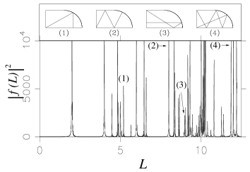
FIG. 1.: $|f(L)|^{2}$ evaluated from the first $9910$ eigenvalues of the desymmetrized stadium billiard with radius $r=1$ and straight line of length $a=1$. The labels over some of the peaks indicate the corresponding periodic orbits shown in the inset.

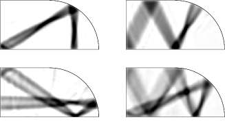
FIG. 2.: Spectral function (Eq. (3)) corresponding to the orbits (1)-(4) (from upper left to bottom right) shown in the inset of Fig. 1. Eq. 4 was evaluated for the first 9910 eigenfunctions of the desymmetrized stadium billiard.

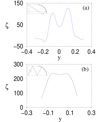
FIG. 3.: Spectral function of the orbit (3) and (2) of Fig. 1 evaluated over the transversal section to the orbits showed in the insets. The transversal coordinate is $y$, with $y=0$ on the orbit.

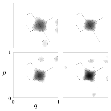
FIG. 4.: Phase space representation of the spectral function for orbit (1) using the first 150, 500, 2000 and 6500 eigenfunctions of the desymmetrized stadium billiard. The stable and unstable manifolds are plotted with points. The coordinate $q$ is the arc length at the boundary normalized by the perimeter of the billiard and $p$ is the fraction of tangential momentum $p$ .

REFERENCES

- [1] M.C.Gutzwiller, Chaos in Classical and Quantum Mechanics (Springer-Verlag, NY, 1990).
- [2] E. Bogomolny, Physica D 31, 169 (1988).
- [3] E. J. Heller, Phys. Rev. Lett. 53, 1515 (1984).
- [4] L. Kaplan and E. J. Heller, Phys. Rev. E 59, 6609 (1999).
- [5] E. Vergini and G. Carlo, (in preparation).
- [6] E. Vergini, J. Phys. A: Math. Gen. 33 4709 (2000). E. Vergini and G. Carlo, J. Phys. A: Math. Gen. 33 4717 (2000).
- [7] S. Nonnenmacher and A. Voros, J. Phys. A: Math. Gen. 30 (1997) 295-315.
- [8] D. Cohen, H. Primack, and U. Smilansky, Annals of Physics 264, 108 (1998).
- [9] D. Wintgen, Phys. Rev. Lett. 58, 1589 (1987).
- [10] L. A. Bunimovich, Comm. Math. Phys. 65, 295 (1979).
- [11] J. M. Tualle and A. Voros, Chaos,Solitons and Fractals 5 1085 (1995).