Divergence Measure Between Chaotic Attractors

Abstract

We propose a measure of divergence of probability distributions for quantifying the dissimilarity of two chaotic attractors. This measure is defined in terms of a generalized entropy. We illustrate our procedure by considering the effect of additive noise in the well known Hénon attractor. Comparison of two Hénon attractors for slighly different parameter values, has shown that the divergence has complex scaling structure. Finally, we show how our approach allows to detect non-stationary events in a time series.

Through the appropriate embedding procedures, strange attractors can be numerically approximated by a large sets of points, either from experimental time series (TS) or from numerical simulation of chaotic systems. Advances in nonlinear analysis of TS have made possible to identify and classify chaotic dynamical systems, to determine if a signal is deterministic or not, and to establish correlations where the traditional linear analysis were not sensitive. However, there are many situations where we need not a complete characterization of an attractor, but rather a quantitative way of comparing attractors. For instance, recently several authors have proposed to use some measures of dissimilarity of attractors to analyze non-stationary signals [1, 2] and for TS classification [3]. In some situations it could be important to quantify the difference of two attractors from the same chaotic dynamical systems, corresponding to slightly different parameters. The computation of the hierarchy of generalized dimensions does not help, because even if all dimensions of two fractal sets are equal, this does not guarantee that the two fractal objects are identical. In order to give a quantitative answer to these issues, a number of dissimilarity measures have been proposed in the literature [2, 4, 5]. The quantitative comparison of attractors can be relevant in many different problems such as: numerical taxonomy of TS; to establish a criterion for stationarity; to study the numerical convergence of chaotic solutions; to evaluate the effect of nonlinear noise reduction of noisy chaotic attractors, among other applications. For the above mentioned purposes we need a reliable way of comparing attractors rather than their detailed characterization. In this paper, we propose a divergence measure based on a generalized entropy function for quantifying the similarity of attractors.

From the information theory viewpoint, the amount of uncertainty of the probability distribution (PD), ${p_{i}}$, is defined in a general way by $H_{f}\left[p_{i}\right]=-\sum_{i}f\left[p_{i}\right]$ [6]. There is not a unique information measure $H_{f}$. The more commonly used information measure or entropy function was introduced by Shannon [7] where $f\left(p\right)=p\ln p$. Generalized entropy $f_{q}$ has been postulated by Rényi [8] and Havrda-Charvát [9]. Rényi’s generalized entropy has been used to define a hierarchy of generalized dimensions [10]. Tsallis introduced the Havrda-Charvát entropy function to elaborate an non-extensive thermodynamics [11]. Associated with an entropy function $f$, we have a divergence measure $D_{f}\left(p:\hat{p}\right)$ between two PD ${p_{i}}$ and $\hat{p}_{i}$. A general divergence measure form associated to the $f$-entropy was given by Csiszár [12]

$$D_{f}\left(p:\hat{p}\right)=\sum_{i}\left(\hat{p}_{i}f\left[\frac{p_{i}}{\hat{p}_{i}}\right]+p_{i}f\left[\frac{\hat{p}_{i}}{p_{i}}\right]\right),$$ (1)

where $f$ is a convex function and one imposes the condition $f\left(1\right)=0$, that guarantees $D_{f}\left(p:p\right)=0$. Rényi’s generalized entropy does not satisfy convexity. Fortunately, Havrda-Charvát entropy function fulfills this property. For this reason we will work here with the Havrda-Charvát entropy function. From here on we shall refer to the generalized divergence measure associated with the Havrda-Charvát entropy function, simply as the $q$-divergence, and will be denoted by $D_{q}$. If we replace $f$ by the function corresponding to the Shannon entropy, we obtain the well known Kullback-Leibler distance [13].

$$D_{1}\left(p:\hat{p}\right)=\sum_{i}\left(p_{i}\ln\left[\frac{p_{i}}{\hat{p}_{i}}\right]+\hat{p}_{i}\ln\left[\frac{\hat{p}_{i}}{p_{i}}\right]\right).$$ (2)

The function $f$ corresponding to the Havrda-Charvát entropy is given by $f_{q}\left(p\right)=\left(q-1\right)^{-1}\left(p^{q}-p\right)$. Then, the associated $q$-distance is given by

$$D_{q}\left(p:\hat{p}\right)=\left(q-1\right)^{-1}\left(\sum_{i}p_{i}^{q}\hat{p}_{i}^{1-q}+\sum_{i}\hat{p}_{i}^{q}p_{i}^{1-q}-2\right).$$ (3)

It is easy to show that $D_{q}\left(p:\hat{p}\right)\rightarrow D_{1}\left(p:\hat{p}\right)$ when $q\rightarrow 1$. The $q$-divergence measure is positive definite, has been made symmetric, and fulfills $D_{q}\left(p:p\right)=0$. Also $D_{q}\left(p:\hat{p}\right)$ considered as a function of ${p_{i}}$ and ${\hat{p_{i}}}$ is convex. We remark that $D_{q}$ is semi-metric, since it may not satisfy the triangular inequality.

After these definitions, let us consider the divergence between two finite time series embedded in ${\cal R}^{d}$, $X=\left({\bf x}_{0},\ldots,{\bf x}_{N}\right)$ and $Y=\left({\bf y}_{0},\ldots,{\bf y}_{N}\right)$. There are two well known ways of estimating the quantities (2) and (3) from $X$ and $Y$. The most straightforward, but also more expensive, is to use a box counting approach: one defines a partition $\Pi_{\varepsilon}$ of the state space, with characteristic size $\varepsilon$. Thus the probability to find a point of $X$ ($Y$) in the $i$th box is $p_{i}$ ($\hat{p}_{i}$). By counting the number of points $n_{i}$ in the box $i$, the probabilities $p_{i}$ can be estimated as $p_{i}=n_{i}/N$, where $N$ is the total number of points. Some authors have refined this procedure, by adapting the size of the boxes depending on the local density [14].

On the other hand, a more efficient method of estimating (2) and (3) is by correlation sums [15]. Instead of taking a fixed mesh, one can calculate the probability $P\left({\bf x}_{j},\varepsilon\right)$ to find a $d$-dimensional point within a sphere of radius $\varepsilon$ centered around the ${\bf x}_{j}$, with $j=1,\ldots,M$ randomly chosen from the trajectory $X$. $P\left({\bf x}_{j},\varepsilon\right)$ is estimated by counting the number $n_{j}$ of points falling in the sphere of radius $\varepsilon$ centered at ${\bf x}_{j}$,

$$P\left({\bf x}_{j},\varepsilon\right)=N^{-1}\sum_{i=1}^{N}\Theta\left(\varepsilon-|{\bf x}_{i}-{\bf x}_{j}|\right)\ \ \ \ j=1,\ldots,M.$$ (4)

In our case the expressions (2) and (3) can be rewritten as

$$D_{1}\left(p:\hat{p},\varepsilon\right)=M^{-1}\left(\sum_{j=1}^{M}\ln\left[\frac{\sum_{i=1}^{N^{\prime}}\Theta\left(\varepsilon-|{\bf y}_{i}-{\bf x}_{j}|\right)}{\sum_{i=1}^{N^{\prime}}\Theta\left(\varepsilon-|{\bf x}_{i}-{\bf x}_{j}|\right)}\right]+\sum_{j=1}^{M}\ln\left[\frac{\sum_{i=1}^{N^{\prime}}\Theta\left(\varepsilon-|{\bf x}_{i}-{\bf y}_{j}|\right)}{\sum_{i=1}^{N^{\prime}}\Theta\left(\varepsilon-|{\bf y}_{i}-{\bf y}_{j}|\right)}\right]\right),$$ (5)

$$D_{q}\left(p:\hat{p},\varepsilon\right)=\frac{M^{-1}}{\left(q-1\right)}\left(\sum_{j=1}^{M}\left(\frac{\sum_{i=1}^{N^{\prime}}\Theta\left(\varepsilon-|{\bf y}_{i}-{\bf x}_{j}|\right)}{\sum_{i=1}^{N^{\prime}}\Theta\left(\varepsilon-|{\bf x}_{i}-{\bf x}_{j}|\right)}\right)^{q}+\sum_{j=1}^{M}\left(\frac{\sum_{i=1}^{N^{\prime}}\Theta\left(\varepsilon-|{\bf x}_{i}-{\bf y}_{j}|\right)}{\sum_{i=1}^{N^{\prime}}\Theta\left(\varepsilon-|{\bf y}_{i}-{\bf y}_{j}|\right)}\right)^{q}-2\right).$$ (6)

Where $\Theta(x)$ is the step function which has the value 1 if $x\geq 0$ and is 0 otherwise, $|{\bf x}_{i}-{\bf y}_{j}|$ is the distance between ${\bf x}_{i}$ and ${\bf y}_{j}$. The sum is taken only for those $i$’s and $j$’s that are separated in time by more than $B$ sampling times to avoid artifactural correlations [16], thus $N^{\prime}=N-d-B$. Notice that the quantities (2) and (3) are defined for two finite discrete probability distributions $p_{i}$ and $\hat{p}_{i}$ only if $p_{i}>0$, and $\hat{p}_{i}>0$, and if there is a one-to-one correspondence between the elements $i$ [8]. In order to satisfy these requirements, we perform the summation in the box counting approach (Eq. (2) and (3)) only over the boxes $i$ that contain points from both $X$ and $Y$ (i.e. $p_{i}>0$ and $\hat{p}_{i}>0$). In the sphere counting scheme (Eq. (5) and (6)), we include in the summation over $j$ only spheres which contain points both in $X$ and $Y$ and for this reason $M$ decreases with $\varepsilon$.

Now, we shall present some examples of numerical computations of the q-divergence $D_{q}$ between two time series. We estimate the $D_{q}$ by means of the two before mentioned methods: the box counting (BC), and the sphere counting (SC). In the case of BC algorithm, for simplicity, we restrict our analysis to dimension $d=2$. As our first example, we deal with trajectories of $10\ 000$ points of the Hénon model $x_{n+1}=1-ax_{n}^{2}+bx_{n-1}$, with parameters $a=1.4$ and $b=0.3$; cf. Kantz [4]. The set $X$ corresponds to the clean attractor, while the set $Y$ consists of the same set of points plus an additive Gaussian noise. In Fig. 1 we present the mean value of $D_{1}$ versus $\varepsilon$ computed with the BC method. We computed the mean value over 5 realizations of $Y$ with signal-to-noise ratio $\eta=20$ dB [17]. Of course, the divergence depends of the length scale $\varepsilon$. By choosing a relatively small $\varepsilon$, $D_{q}$ will pick up local differences between $X$ and $Y$. However, taking $\varepsilon$ too small leads to poor statistics. For large $\varepsilon$, we lose the small scale structure of the attractors that they become indistinguishable. We can see that $D_{1}$ reaches a maximum at a values of $\varepsilon$ that will be denoted by $\varepsilon_{0}$. The dashed curve corresponds to $S=\langle D_{1}\rangle/\sigma\left(D_{1}\right)$ where $\langle\rangle$ denotes the mean value over 5 realizations and $\sigma$ denote the standard deviation. We can see that the maximum value of $D_{1}$ presents very good statistics.

In Fig. 2 we display the $q$ dependence of $D_{q}\left(\varepsilon_{0}\right)$ for different noise level ($\eta=30$ dB in solid line, $\eta=20$ dB in dashed line and $\eta=10$ dB in dotted line). As shown in Fig. 2, the parameter $q$ is like a gain control parameter. The divergence of the two attractors increases with $q$. This fact can be used to detect small divergence as we will discuss in the last example. In Fig. 3 we illustrate the behavior of the mean value of $D_{2}$ versus $\varepsilon$ computed with SC method. We computed the mean value over 5 realization of $Y$ for each level of noise. We can see that $D_{2}$ presents a maximum at $\varepsilon_{0}$ which depends on the characteristic length scale at which the attractors differ. The $\varepsilon$ dependence of $D_{q}$ characterizes the relationship between the sets $X$ and $Y$. In the case analyzed here, this length scale is related to the level of noise added to $X$. In Fig. 4 we display $D_{2}\left(\varepsilon_{0}\right)$ versus $\eta$. This figure shows that the $D_{2}\left(\varepsilon_{0}\right)$ scales exponentially with the level of noise added to the signal.

Now, we compare two clean Hénon attractors for slightly different parameter values. In this case $Y$ corresponds to parameters $a=1.35$ and $b=0.31$, while $X$ remains the same. In Fig. 5 we display $D_{1}$ computed with $N=50\ 000$ points, embedding dimension $d=2$, using the BC method (dotted line), using the SC method (dashed line), and with $d=3$ using the BC method (solid line). When we compare these attractors, we find that the divergence measure as a function of $\varepsilon$ exhibits a more complex scaling structure than showed in the previous example. This complex relationship between the attractors has not been reported in early studies [4, 18].

Let us finally show how the $q$-distance $D_{q}$ can be used to detect non stationarity events in a TS. As numerical example, let us consider a generalized baker map defined by

$$v_{n}\leq\alpha:\ \ \ \ u_{n+1} = \beta u_{n},\ \ \ \ \ \ \ \ \ \ \ \ \ v_{n+1}=v_{n}/\alpha,$$ (7)

$$v_{n}>\alpha:\ \ \ \ u_{n+1} = 0.5+\beta u_{n},\ \ \ \ \ v_{n+1}=\frac{v_{n}-\alpha}{1-\alpha}.$$ (8)

For this map, the parameter $\beta$ can be varied without changing the positive Lyapunov exponent. We generate a non stationary TS of length 8192 points with $\alpha=0.4$ and two values of $\beta$. In the first 4096 iterations we use $\beta=0.6$, and in the second 4096 iterations we set $\beta=0.8$. We record $u+v$, then we subtract the mean value and normalize to unit variance separately each one of the two parts; cf. Schreiber [2]. Thus, we have a non stationary event in the middle of the TS that is very hard to detect, because observables like mean, variance and maximal Lyapunov exponent are constant by construction. Figure 6 shows $D_{2}\left(S_{i}:S_{j}\right)$ and $D_{6}\left(S_{i}:S_{j}\right)$, between two nearest non-overlapping segments $S_{i}$ and $S_{j}$ of 1000 points [19]. This example shows also that the parameter $q$ plays a role of a nonlinear gain parameter. We can see that for $q=6$ the divergence was able to detect precisely when the small change in $\beta$ ocurr, while for $q=2$ we have a poor discrimination power. We used resolution $\varepsilon=0.1155$ in the computation. We have a window resolution with similar results for $\varepsilon$ in $[0.075,0.15]$.

We have introduced the $q$-divergence as a measure of dissimilarity of two finite sets. Our approach is particularly useful for comparing attractors. We found that the divergence decreases exponentially when $\eta$ increases. Comparison of two Hénon attractors for slighly different parameter values has shown that the $q$-divergence has a complex scaling structure. Also this tool promises to be useful for detecting non-stationary event in a TS, even in very hard conditions. Thus It will be seen that some interesting physical insight is gained by recourse to this type of dissimilarity measure.

The author acknowledges the financial support of FAPESP Grant N^o 99/07186-3. The author thank C.P. Malta for a careful reading of the manuscript and her useful comments.

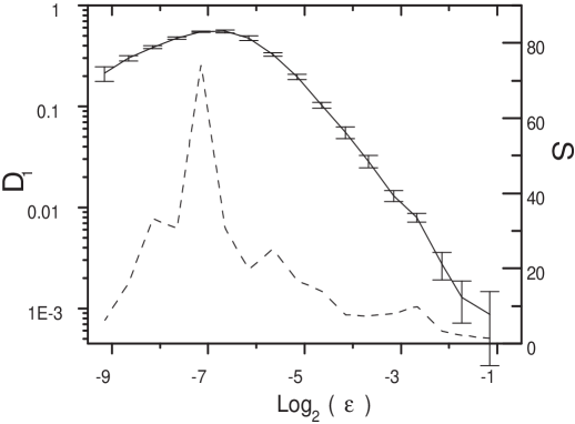
FIG. 1.: Solid Line: $D_{1}\left(\varepsilon\right)$ between the TS $X$ generated by the Hénon system and the TS $Y$ generated by the same systems contaminated with noise ($\eta=20$ dB), computed with the BC scheme using $N=10\ 000$ points and $d=2$ (left axis). Dashed line: the statistic $S\left(\varepsilon\right)$ (right axis).

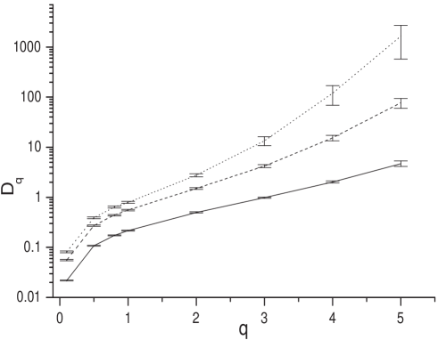
FIG. 2.: The $q$-distance $D_{q}\left(\varepsilon_{0}\right)$ between the TS $X$ generated by the Hénon system and the TS $Y$ generated by the same systems contaminated with several level of noise as a function of the parameter $q$ (solid line: SNR= 30 dB, dashed line: $\eta=20$ dB and dotted line $\eta=10$ dB) . The calculation were performed with the BC scheme using $N=10\ 000$ points and $d=2$.

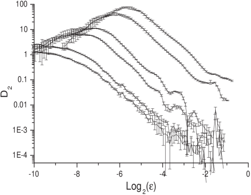
FIG. 3.: Distance $D_{2}$ between Hénon system and itself contaminated with several level of noise (between $\eta=30$ dB to $\eta=7$ dB). The calculation were performed with the SC scheme using $N=10\ 000$ points, $B=20$ and $d=2$.

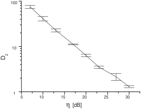
FIG. 4.: Divergence $D_{2}\left(\varepsilon_{0}\right)$ between Hénon system and itself contaminated with noise as a function of the level of noise $\eta$.

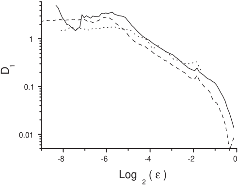
FIG. 5.: Estimated values of $D_{1}$ as a function of $\varepsilon$ for two time series of length $N=50\ 000$, and $B=20$ generated by slightly different Hénon systems. Dotted line: using BC method with $d=2$. Dashed line: using SC method with $d=2$. Solid line: using SC method with $d=3$.

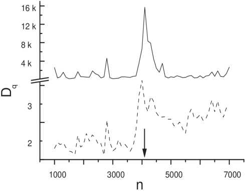
FIG. 6.: $D_{6}$ (solid line) and $D_{2}$ (dashed line) between two non-overlapping subsequent segments of TS with a non-stationary event at 4096.

REFERENCES

- [1] R. Manuca and R. Savit, Physica D 99, 134 (1996).
- [2] T. Schreiber, Phys. Rev. Lett. 78, 843-847 (1997).
- [3] T. Schreiber and A. Schmitz, Phys. Rev. Lett. 79 1475-1478 (1997).
- [4] H. Kantz, Phys. Rev. E 49, 5091-5097 (1994).
- [5] A.M. Albano, P.E. Rapp and A. Passamante, Phys. Rev. E. 52, 196-206 (1995).
- [6] J. Aczél and Z. Daròczy, On mesures of Information and Their Characterizations (Academic Press, Mathematics in Science and Engineering, vol 115, 1975)
- [7] C.E. Shannon and W. Weaver, The Mathematical Theory of Communication (University of Illinois Press, Chicago, 1949).
- [8] A. Rényi, Probability Theory, (North-Holland, Amsterdam, 1970).
- [9] M.E. Havrda and F. Charvát, Kybernetica 3, 30-35 (1967).
- [10] P. Grassberger, Phys. Lett. A 97, 227-230 (1983).
- [11] C. Tsallis, J. Stat. Phys. 52, 479 (1988).
- [12] I. Csiszár, Periodica Math. Hungarica 2, 191-213 (1972).
- [13] S. Kullback, Information Theory and Statistics, J. Wiley, New York, (1959).
- [14] A.M. Fraser and H.L. Swinney, Phys. Rev. A 33, 1134-1140 (1986).
- [15] P. Grassberger and I. Procaccia, Phys. Rev. Lett. 50, 346 (1983).
- [16] J. Theiler, Phys. Rev. A 34, 2427 (1986).
- [17] The signal-to-noise ratio in decibels (dB) is defined as .
- [18] C. Diks, W.R. van Zwet, F. Takens and J. DeGoede. Phys. Rev. E 53, 2169-2176 (1996).
- [19] The total signal of 8192 points is split into 71 segments of 1000 points with 900 points of overlapping. Thus .