Second quantization approach to characteristic polynomials in RMT

Abstract

The distribution of the characteristic polynomial $Z(U,\theta)$ of $N\times N$ matrices $U$ in the Circular Unitary Ensemble is studied by the method of second quantization for one-dimensional fermions. For infinite $N$ the Gaussian distribution of $Z(U,\theta)$ is established straightforwardly by bosonization. A general expression for the $n$-point correlation function of the characteristic polynomial at different points is given by this method. The case of finite $N$ is discussed.

The statistical properties of the Riemann zeta function [1] have been extensively studied analytically [2, 3] and numerically [4] and their analogy with the corresponding properties of ensembles of random matrices was investigated within the framework of the random matrix theory [5]. Recently, the distribution of values taken by the characteristic polynomials

$$Z(U,\theta)=\det\left(I-Ue^{i\theta}\right)=\prod_{j=1}^{N}\left(1-e^{i(\theta-\theta_{j})}\right)$$ (1)

of $N\times N$ unitary random matrices $U$ with eigenvalues $e^{-i\theta_{j}}$ belonging to the circular unitary ensemble (CUE) was investigated in [6, 7]. In particular, it was shown by explicit calculations that in the limit $N\rightarrow\infty$ the distribution of real and imaginary part of $\log Z(U,\theta)$ divided by a factor $\sqrt{(1/2)\log N}$ is a standard normal distribution in two dimensions. This was conjectured to mimic the similar behavior of the Riemann zeta function high up the critical line. The convergence of the corresponding cumulants to the gaussian limit as $N\rightarrow\infty$ was also explicitly calculated and they were conjectured to describe the corresponding properties of the Riemann zeta function.

In this paper I use the equivalence between the CUE and a theory of fermions in one dimension to calculate the statistical properties of $\log Z(U,\theta)$ using the method of second quantization. One of the most prominent features of this approach is that the case $N=\infty$ can be studied from the very beginning, thus avoiding the tedious finite $N$ calculations and the asymptotic expansion. For infinite $N$ the calculations simplify a lot, since in this case the fermionic theory is equivalent to a theory of free bosons, the fact known under the name of bosonization [8]. In what follows I calculate the distribution functional of the characteristic polynomial (1) for infinite $N$ using this equivalence. In mathematical literature the bosonization is known under the name of Frobenius formula for irreducible characters of the permutation group [9] or Szegö asymptotic formula for Toeplitz determinants.

Let me briefly describe the relation between the CUE and the fermions in one dimension. In the random matrix theory one is interested mainly in calculating statistical averages of functions, which depend only on the eigenvalues $e^{-i\theta_{j}}$ of $U$. Consider some symmetric function of eigenvalues $f(\theta)\equiv f(\theta_{1},\ldots,\theta_{N})$, and its average, defined as

$$\langle f\rangle\equiv\frac{1}{(2\pi)^{N}N!}\int d^{N}\theta\,\,\left|D\left(e^{i\theta}\right)\right|^{2}f(\theta),$$ (2)

where the (Haar) measure of integration is defined with help of the Vandermonde determinant [9, 5]:

$$D(z)\equiv D(z_{1},\ldots,z_{N})=\det\left[z_{j}^{N-k}\right]_{j,k=1,2,\ldots,N}=\prod_{j<k}(z_{j}-z_{k})$$ (3)

Consider a quantum particle on a ring $0<\theta<2\pi$, described by the wave-function of the $n$-th orbital:

$$\psi_{n}(\theta)=\frac{1}{\sqrt{2\pi}}e^{in\theta}.$$ (4)

The Vandermonde determinant $D\left(e^{i\theta}\right)$ is therefore proportional to the Slater determinant:

$$\Psi(\theta)\equiv\Psi_{0}(\theta_{1},\ldots,\theta_{N})=\frac{1}{\sqrt{(2\pi)^{N}N!}}\det\left(e^{i(N-k)\theta_{j}}\right)$$ (5)

composed of particles (fermions) occupying the orbitals $n=N-k=0,\ldots,N-1$. The proportionality factor coincides exactly with the square root of the normalization factor in front of the integral in (2) and this average can be rewritten as a quantum-mechanical expectation value:

$$\langle f\rangle=\langle\Psi_{0}|f\,|\Psi_{0}\rangle=\int d^{N}\theta\,\,\Psi_{0}^{*}(\theta)\,f(\theta)\,\Psi_{0}(\theta)$$ (6)

of the operator $f$ defined as $f(\theta)$ in the coordinate representation. This correspondence of the RMT and one-dimensional fermions will be used extensively throughout the paper and in particular the statistical average $\langle\ldots\rangle$ and the quantum expectation value $\langle\Psi_{0}|\ldots|\Psi_{0}\rangle$ will be interchanged in the course of the paper by the virtue of (6). Some application of the fermionic picture will be presented in what follows.

The central object of my discussion is the logarithm of the characteristic polynomial (1):

$$L(\theta)=\log Z(U,\theta)=\sum_{j=1}^{N}\log\left(1-e^{i(\theta-\theta_{j})}\right).$$ (7)

Expanding the logarithm, the equation (7) can be rewritten as

$$L(\theta)=-\sum_{k=1}^{\infty}\frac{e^{ik\theta}}{k}\sum_{j=1}^{N}e^{-ik\theta_{j}}=-\sum_{k=1}^{\infty}\frac{e^{ik\theta}\rho_{k}}{k},$$ (8)

where we have used the Fourier transform of the density operator:

$$\rho_{k}=\mbox{tr}\,\left(U^{k}\right)=\sum_{j=1}^{N}e^{-ik\theta_{j}}=\int_{0}^{2\pi}\!d\theta\,e^{-ik\theta}\rho(\theta),\;\;\;\;\;\;\;\rho(\theta)=\sum_{j=1}^{N}\delta(\theta-\theta_{j})=\frac{1}{2\pi}\sum_{k=-\infty}^{+\infty}e^{ik\theta}\rho_{k}.$$ (9)

In order to calculate the statistical properties of $L(\theta)$ using the correspondence (6) between statistical average and quantum expectation value it is convenient to employ the method of second quantization. We introduce creation and annihilation operators $c^{\dagger}_{n}$ and $c_{n}$ for a fermion on the $n$-th orbital with usual anti-commutation relations:

$$\{c_{n},c^{\dagger}_{m}\}\equiv c_{n}c^{\dagger}_{m}+c^{\dagger}_{m}c_{n}=\delta_{n,m},\;\;\;\;\;\{c_{n},c_{m}\}=\{c^{\dagger}_{n},c^{\dagger}_{m}\}=0$$ (10)

The quantum state $|\Psi_{0}\rangle$ is then defined by the action of the creation operators on the vacuum:

$$|\Psi_{0}\rangle=\prod_{n=0}^{N-1}c^{\dagger}_{n}|\mbox{Vac}\rangle.$$ (11)

The second-quantized form of the density operator $\rho_{k}$ is given by the standard rules [10]:

$$\rho_{k}=\rho^{\dagger}_{-k}=\sum_{n=-\infty}^{+\infty}c^{\dagger}_{n-k}c_{n}$$ (12)

for $k\neq 0$, while for $k=0$ the definition (9) gives $\rho_{0}=N$ — the total number of particles. When acting on the state $|\Psi_{0}\rangle$ the density operator $\rho_{k}$ creates a linear combination of states in which one particle on the $n$-th orbital is moved $k$ orbitals down, provided the orbital $n-k$ is empty. This simple observation yields the important result (for $k\neq 0$):

$$\langle\rho_{k}\rho^{\dagger}_{p}\rangle=\delta_{k,p}C_{2}(k)=\delta_{k,p}\langle\Psi_{0}|\rho_{k}\rho^{\dagger}_{k}|\Psi_{0}\rangle=\delta_{k,p}\times\left\{\begin{array}[]{cc}|k|,&|k|\leq N\\ N,&|k|>N\end{array}\right.$$ (13)

otherwise obtained by using the Wick theorem. The correlation function $C_{2}(k)=\langle\rho_{k}\rho^{\dagger}_{k}\rangle$ with $C_{2}(0)=N^{2}$, is nothing but a Fourier transform of DOS-DOS correlation function [5] of CUE :

$$C_{2}(\theta;N)=\langle\rho(\theta)\rho^{\dagger}(0)\rangle=\frac{1}{2\pi}\sum_{k=-\infty}^{+\infty}e^{ik\theta}C_{2}(k;N)=\frac{N}{2\pi}\delta(\theta)+\left(\frac{N}{2\pi}\right)^{2}-\left(\frac{\sin\frac{N\theta}{2}}{2\pi\sin\frac{\theta}{2}}\right)^{2}.$$ (14)

The symmetry of the correlation function $C_{2}(k;N)$ with respect to $k\rightarrow-k$ follows from the fact that for finite $N$ the density operators $\rho_{k}$ and $\rho^{\dagger}_{k}$ commute. For infinite $N$, as we shall see, this is not true.

I now proceed to calculate the correlation functions of the logarithm of the characteristic polynomial. In the work [6] the correlation functions of $L(\theta)$ were calculated at the same point. Here I generalize this result, to the case of the two-point correlation function, and calculate

$$K_{2}(\theta_{1}-\theta_{2};N) = \langle L(\theta_{1})L^{\dagger}(\theta_{2})\rangle$$ (15)

$$P_{2}(\theta_{1}-\theta_{2};N) = \langle L(\theta_{1})L(\theta_{2})\rangle.$$ (16)

where in the coordinate representation $L^{\dagger}(\theta)=L^{*}(\theta)$.

Due to the translational symmetry all the correlation functions depend on the difference $\theta=\theta_{1}-\theta_{2}$ only. From (15) and (16) the correlation functions of real and imaginary part of $L(\theta)$ can be easily obtained. I notice that $P_{2}(\theta)$ vanishes due to the fact that the Kronecker delta in (13) is never satisfied. Moreover, it follows that

$$Q_{2}(\theta_{1}-\theta_{2};N) \equiv \langle\mbox{Re}\,L(\theta_{1})\,\mbox{Re}\,L(\theta_{2})\rangle=\frac{\mbox{Re}\,K_{2}(\theta_{1}-\theta_{2};N)}{2}$$

$$R_{2}(\theta_{1}-\theta_{2};N) \equiv \langle\mbox{Im}\,L(\theta_{1})\,\mbox{Im}\,L(\theta_{2})\rangle=\frac{\mbox{Re}\,K_{2}(\theta_{1}-\theta_{2};N)}{2}$$ (17)

and in addition there exists a cross-function given by

$$X_{2}(\theta_{1}-\theta_{2};N)\equiv\langle\mbox{Im}\,L(\theta_{1})\,\mbox{Re}\,L(\theta_{2})\rangle=-\langle\mbox{Re}\,L(\theta_{1})\,\mbox{Im}\,L(\theta_{2})\rangle=\frac{\mbox{Im}\,K_{2}(\theta_{1}-\theta_{2};N)}{2}$$ (18)

It can be checked that $\langle L(\theta)\rangle=\langle L^{\dagger}(\theta)\rangle=0$ so there is no difference between connected and disconnected correlation functions.

The calculation of $K_{2}(\theta;N)$ using the definition (8) is straightforward:

$$K_{2}(\theta_{1}-\theta_{2};N)=\sum_{k,p=1}^{\infty}\frac{e^{ik\theta}}{kp}\langle\rho_{k}\rho^{\dagger}_{p}\rangle=\sum_{k=1}^{\infty}\frac{e^{ik\theta}}{k^{2}}C_{2}(k;N)=\sum_{k=1}^{N}\frac{e^{ik\theta}}{k}+N\sum_{k=N+1}^{\infty}\frac{e^{ik\theta}}{k^{2}}$$ (19)

For correlations at the same point, $\theta=0$, the result is real and its half coincides precisely with the expression (43) in [6]:

$$\frac{K_{2}(0;N)}{2}=Q_{2}(0;N)=R_{2}(0;N)=\frac{1}{2}\sum_{k=1}^{N}\frac{1}{k}+\frac{N}{2}\sum_{k=N+1}^{\infty}\frac{1}{k^{2}}$$ (20)

which behaves as $(1/2)\log N$ for large $N$. It is worth noticing that for $\theta\neq 0$ the function $K_{2}(\theta)$ is complex, therefore there exists correlation between real and imaginary parts of $L(\theta)$ at different points, a fact which is missed when the correlation function is calculated at the same point.

Now the calculations for the whole distribution of $L(\theta)$ and $L^{\dagger}(\theta)$, equivalent to the distribution of $\mbox{Re}\,L(\theta)$ and $\mbox{Im}\,L(\theta)$ is presented. In order to be able to calculate general $n$-point correlation functions, one has to consider the following generating functional:

$$\Xi[s,s^{*}]=\left\langle\exp\left\{\int_{0}^{2\pi}\frac{d\theta}{2\pi}\left[s^{*}(\theta)L(\theta)+s(\theta)L^{\dagger}(\theta)\right]\right\}\right\rangle$$ (21)

where $s(\theta)$ and $s^{*}(\theta)$ are the source terms. Any $n$-point correlation function can be represented as a functional derivative of $\Xi[s,s^{*}]$:

$$\langle L(\theta_{1})L(\theta_{2})\ldots L^{*}(\theta_{m})L^{*}(\theta_{m+1})\ldots\rangle=\left.\frac{\delta}{\delta s^{*}_{1}}\frac{\delta}{\delta s^{*}_{2}}\ldots\frac{\delta}{\delta s_{m}}\frac{\delta}{\delta s_{m+1}}\ldots\Xi[s,s^{*}]\right|_{s,s^{*}=0}$$ (22)

where $s_{m}$, $s^{*}_{l}$ stand for $s(\theta_{m})$ and $s^{*}(\theta_{l})$ respectively. Using the Fourier transform of these source terms

$$s_{k}=\int_{0}^{2\pi}d\theta\,e^{-ik\theta}s(\theta)\;,\;\;\;\;\;\;s^{*}_{k}=(s_{k})^{*}$$ (23)

and the expression (8) the generating functional (21) can be rewritten as

$$\Xi[s,s^{*}]=\left\langle\exp\left\{-\sum_{k=1}^{\infty}\frac{1}{k}\left(s^{*}_{k}\rho_{k}+s_{k}\rho^{\dagger}_{k}\right)\right\}\right\rangle.$$ (24)

It will be calculated in the limit $N=\infty$. It is convenient to redefine the numbering of one-particle orbitals so the upper occupied level in $|\Psi_{0}\rangle$ corresponds now to $n=0$ and all the states with $n\leq 0$ are occupied. This state is the infinitely deep Fermi sea — the ground state of the fermionic system, if one-particle energy $E_{n}$ is an increasing function of the level index $n$. In addition, this state is now annihilated by the action of $\rho_{k}$ for $k>0$: it is impossible to promote a fermion from the state $n$ to an empty lower state $n-k$. It is well known from the theory of one-dimensional correlated electrons [12] that the operators $\rho_{k}$ and $\rho^{\dagger}_{k}$ acquire non-zero commutation relations in the presence of infinite filled Fermi sea (Schwinger terms). To show it let us begin with

$$[\rho_{k},\rho^{\dagger}_{p}]=\sum_{n,m=-\infty}^{+\infty}[c^{\dagger}_{n-k}c_{n},c^{\dagger}_{m+p}c_{m}]=\sum_{n=-\infty}^{+\infty}\left(c^{\dagger}_{n-k}c_{n-p}-c^{\dagger}_{n-k+p}c_{n}\right)\;.$$ (25)

The result is nonzero, since the operators are not well-behaved. It is necessary to extract the singular part by introducing the normal ordered operators in the state $|\Psi_{0}\rangle$ by extracting the expectation value in this state:

$$:c^{\dagger}_{m}c_{n}:=c^{\dagger}_{m}c_{n}-\langle c^{\dagger}_{m}c_{n}\rangle=c^{\dagger}_{m}c_{n}-\delta_{m,n}n^{0}_{m}\;,$$ (26)

where $n^{0}_{m}\equiv\langle c^{\dagger}_{m}c_{m}\rangle$ is the Fermi-Dirac distribution of occupation numbers in the ground state. Rewriting $c^{\dagger}_{m}c_{n}=:c^{\dagger}_{m}c_{n}:+\delta_{m,n}n^{0}_{m}$ and substituting it into (25) the commutation relation of density operators becomes

$$[\rho_{k},\rho^{\dagger}_{p}]=\sum_{n=-\infty}^{+\infty}\left(:c^{\dagger}_{n-k}c_{n-p}:-:c^{\dagger}_{n-k+p}c_{n}:\right)+\delta_{k,p}\sum_{n=-\infty}^{+\infty}\left(n^{0}_{n-k}-n^{0}_{n}\right)=k\,\delta_{k,p}\;.$$ (27)

In this expression the normal ordered operators were canceled, since they are not singular. The last sum equals to the number of orbitals from $1$ to $k$.

When calculating the matrix elements as in (24) the order of $\rho_{k}$ and $\rho^{\dagger}_{k}$ is important when these operators do not commute. One requires that the matrix element should coincide with the statistical average in the coordinate representation (2). Suppose that an operator $\rho_{k}$ for $k>0$ happens to be next to the left of the state $|\Psi_{0}\rangle$. The result would be zero, since this state is annihilated by $\rho_{k}$ for $k>0$, which is not true for the statistical average. In order to obtain the correct expression all operators $\rho_{k}$ for $k>0$ must be placed to the left of $\rho^{\dagger}_{k}$ for $k>0$, in the so-called anti-normal order. The operators in the generating functional (24) must be therefore rearranged as

$$\Xi[s,s^{*}]=\left\langle\exp\left(-\sum_{k=1}^{\infty}\frac{s^{*}_{k}\rho_{k}}{k}\right)\exp\left(-\sum_{k=1}^{\infty}\frac{s_{k}\rho^{\dagger}_{k}}{k}\right)\right\rangle$$ (28)

Using the fact that the commutator of $\rho_{k}$ and $\rho^{\dagger}_{k}$ is a $c$-number and $\rho_{k}$ annihilates the ground state for $k>0$, the generating functional is given by the famous Baker-Campbell-Hausdorff formula:

$$\Xi[s,s^{*}] = \left\langle\exp\left(-\sum_{k=1}^{\infty}\frac{s^{*}_{k}\rho_{k}}{k}\right)\exp\left(-\sum_{k=1}^{\infty}\frac{s_{k}\rho^{\dagger}_{k}}{k}\right)\right\rangle=\exp\left(\sum_{k=1}^{\infty}\frac{s^{*}_{k}s_{k}}{k^{2}}[\rho_{k},\rho^{\dagger}_{k}]\right)$$ (29)

$$= \exp\left(\sum_{k=1}^{\infty}\frac{s^{*}_{k}s_{k}}{k}\right)$$

which is obviously gaussian. In particular, taking the corresponding derivatives of $\Xi[s,s^{*}]$ with respect to $s_{k}/k$ and $s^{*}_{k}/k$ in analogy to (22) the correlation function of powers of of $\rho_{k}$ or traces of $U^{k}$ can be calculated:

$$\left\langle\prod_{k}{\rho^{\dagger}_{k}}^{m_{k}}\prod_{p}\rho_{p}^{m^{\prime}_{p}}\right\rangle=\left\langle\prod_{k}\left(\mbox{tr}\,{U^{\dagger}}^{k}\right)^{m_{k}}\prod_{p}\left(\mbox{tr}\,U^{p}\right)^{m^{\prime}_{p}}\right\rangle=\prod_{k}\delta_{m_{k},m^{\prime}_{k}}k^{m_{k}}m_{k}!$$ (30)

in accordance with the results of [13]. This result and the gaussian characteristic functional (29) are consequences of the anomalous commutation relations (27) that are fulfilled by the operator $\rho_{k}$ and its hermitean conjugate and the fact that $\rho_{k}$ annihilates the ground state for $N=\infty$. It is worth mentioning here that the correlation function (30) and its generating functional (29) are in fact the restatements in terms of the field theory of the so called functional central limit theorem for $\log Z$ discussed in [7]. There it was proven using the Frobenius formula for the irreducible characters of the permutation group, which constitutes the mathematical basis of the bosonization [8].

Returning to the function $s(\theta)$ of the angle, the bilinear form in the exponent of (29) can be rewritten as a double integral

$$\log\Xi[s,s^{*}]=\int_{0}^{2\pi}\int_{0}^{2\pi}\frac{d\theta_{1}}{2\pi}\frac{d\theta_{2}}{2\pi}\,s^{*}(\theta_{1})\,K_{2}(\theta_{1}-\theta_{2};\infty)\,s(\theta_{2})\,,$$ (31)

where the “propagator” is given by (19) for infinite $N$, i.e.

$$K_{2}(\theta;\infty)=\sum_{k=1}^{\infty}\frac{e^{ik\theta}}{k}e^{-2k\eta}=-\log\left(1-e^{i\theta}e^{-2\eta}\right)$$ (32)

and the infinitesimal imaginary part $\eta$ of the angle $\theta$ was included to ensure convergence at $\theta=0$. It was not necessary for finite $N$, since in (19) the first sum is finite and the second one is absolutely convergent. It is well known [8, 12] that an ultraviolet cut-off $1/\eta$ should be introduced when dealing with an infinite Fermi sea. Using this cut-off, the correlation function (32) at the same point ($\theta=0$) is described by

$$K_{2}(0;\infty)=-\log\left(1-e^{-2\eta}\right)\approx\log\frac{1}{2\eta},$$ (33)

which should be compared with the leading behavior of $K_{2}(0;N)\sim\log N$. In fact, for large but finite $N$ one can make the scaling ansatz for the correlation function $K_{2}(0;N,\eta)$:

$$K_{2}(0;N,\eta)=\log\frac{1}{2\eta}\times f\left({\log N}/{\log\frac{1}{2\eta}}\right)$$ (34)

with $f(x)\rightarrow 1$ as $x\rightarrow\infty$ and $f(x)\approx x$ for $x\rightarrow 0$. The scaling form (34) can be justified by calculating the leading behavior of (19) for $N\rightarrow\infty$ and $\theta=2i\eta\rightarrow 0$. Using the scaling (34) the correspondence between $N$ and $1/2\eta$ is established for the leading behavior (in $\log N$) of the second moments of $\mbox{Re}\,L(\theta)$ and $\mbox{Im}\,L(\theta)$ at the same point. Whether the bosonization, which applies for the case $N=\infty$ only, can provide results for other correlation functions for finite $N$ through some scaling relations like (34) is an open question.

Finally I give explicit expressions for correlation functions $Q_{2}$, $R_{2}$ and $X_{2}$ for $\theta\neq 0$ calculated using (17,18). Separating the real and imaginary parts in (32) they read:

$$Q_{2}(\theta;\infty)=R_{2}(\theta;\infty)=\frac{1}{2}\log\left(\frac{1}{\left|2\sin\frac{\theta}{2}\right|}\right)$$ (35)

$$X_{2}(\theta;\infty)=\frac{\theta-\pi}{4}\;\mbox{mod}\,\frac{\pi}{2}$$ (36)

where the $\mbox{mod}\,\pi/2$ means that the values taken by $X_{2}(\theta;\infty)$ lie in the interval $[-\pi/4,\pi/4]$ so it is a periodic function of the angle. The functions (35,36) are shown in Figure 1. It would be interesting to compare these correlation functions with the corresponding functions for real and imaginary parts of the Riemann zeta function high up the critical line. The function $R_{2}(\theta;\infty)$ is related to the variance of number of eigenvalues in the arc of length $\theta$ which was studied in [11].

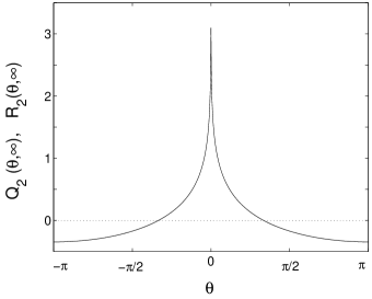
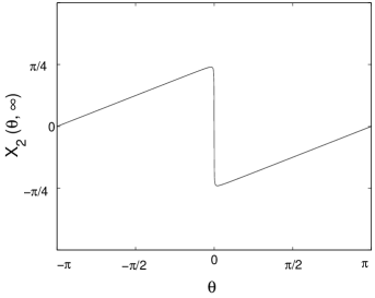
Figure 1: The correlation functions $Q_{2}(\theta;\infty)$, $R_{2}(\theta;\infty)$ and $X_{2}(\theta;\infty)$ for $\eta=0.001$.

In this paper I have shown how the one to one correspondence between the probability measure and Slater determinants of fermions in one dimension can be used in order to calculate different statistical properties of Circular Unitary Ensemble of random matrices. In particular, the correlation functions of the density of states, which corresponds to the density of the fermions are obtained with help of the Wick theorem as a diagrammatic expansion. This method was applied to the calculation of correlation functions of characteristic polynomials. The case of $N=\infty$ was treated by the method of bosonization and the generating functional of correlation functions was calculated exactly yielding an alternative derivation of some of the results of [6, 7, 11, 13]. The corresponding distribution was shown to be gaussian corresponding to the functional central limit theorem of [7]. In the future it would be interesting to investigate by the present method the case of finite $N$ in order to obtain the correlation functions of the characteristic polynomials at the same point.

In conclusion I would like to remark that the finite $N$ calculations presented in this paper and in [6, 7, 11, 13] are related to the results obtained for the (static) correlation functions of strongly correlated particles in one dimension. Indeed, it is known that the different circular ensembles of random matrices correspond to the Calogero-Sutherland model [14], which describes a system of $N$ interacting particles. This model with interactions falling off as the inverse square of the distance between the particles and proportional to the coupling constant $\lambda$, was shown in [15] to be equivalent to the system of effective free particles with fractional quantum statistics. The values of the coupling constant $\lambda=1/2$, $1$ and $2$ correspond to the orthogonal, the unitary and the symplectic ensemble respectively. In the present work only the $\lambda=1$ Calogero-Sutherland model equivalent to the free fermions was considered within the framework of the second quantization. The generalization of the present approach to other ensembles, corresponding to more exotic fractional statistics would be an interesting issue.

I would like to thank BRIMS Hewlett-Packard Labs in Bristol for hospitality. I am grateful to J.P. Keating for fruitful, stimulating discussions. I am also grateful to S. Fishman for his comments and generous help during the preparation of this manuscript. This research was supported in part by the U.S.–Israel Binational Science Foundation (BSF), by the Minerva Center for Non-linear Physics of Complex Systems, by the Israel Science Foundation, by the Niedersachsen Ministry of Science (Germany) and by the Fund for Promotion of Research at the Technion.

References

• [1] E.C. Titchmarsh, The theory of the Riemann Zeta Function (Clarendon Press, Oxford, 1986).
• [2] H.L. Montgomery, Proc. Symp. Pure Math. 24, 181, (1973)
• [3] P. Sarnak, Curr. Dev. Math. 84, (1997)
• [4] A.M. Odlyzko, preprint (1989)
• [5] M.L. Mehta, Random Matrices (Academic Press, London, 1991).
• [6] J.P. Keating and N.C. Snaith, Commun. Math. Phys 214, 57, (2000).
• [7] C.P. Hughes, J.P. Keating and Neil O’Connel, preprint, 1999
• [8] For a review see: M. Stone, Bosonization (World Scientific, 1994).
• [9] D.E. Littlewood, The Theory of Group Characters and Matrix Representations of Groups (Clarendon Press, Oxford, 1958).
• [10] J.W. Negele and H. Orland, Quantum Many-Particle Systems (Addison-Wesley, 1995).
• [11] E.M. Rains, Probab. Theor. 107, 219, (1997).
• [12] F. D. M. Haldane, J. Phys. C 14, 2585, (1981)
• [13] P. Diaconis and M. Shashahani, J. Appl. Probab. 31A, 49, (1981)
• [14] F. Calogero, J. Math. Phys. 10, 2191 (1969); B. Sutherland, Phys. Rev. A4, 2019 (1971).
• [15] Z.N.C. Ha, cond-mat/9410101