Vertical transmission of culture and the distribution of family names

Abstract

A stochastic model for the evolution of a growing population is proposed, in order to explain empirical power-law distributions in the frequency of family names as a function of the family size. Preliminary results show that the predicted exponents are in good agreement with real data. The evolution of family-name distributions is discussed in the frame of vertical transmission of cultural features.

,

1 Introduction

The fascinating complexity of social phenomena is increasingly attracting the attention of physicists. We find in the techniques of Statistical Physics an ideal tool for the study of models of such phenomena, where complex “macroscopic” behaviour emerges spontaneously as the consequence of relatively simple “microscopic” dynamical rules. During the last decade, in fact, much work along those lines has been devoted to the study of statistical properties of dynamical processes in economics [1, 2]. Other key social processes—such as the dynamics of cultural features—have received relatively less attention, in spite of the fact that empirical data call for the kind of approach already employed with economical systems. Consider, for instance, the size distribution of large religious groups, shown in Fig. 1. A well defined power-law decay, spanning more that two orders of magnitude, is apparent. These power-law distributions are indeed a main clue to complexity in real and model systems [2].

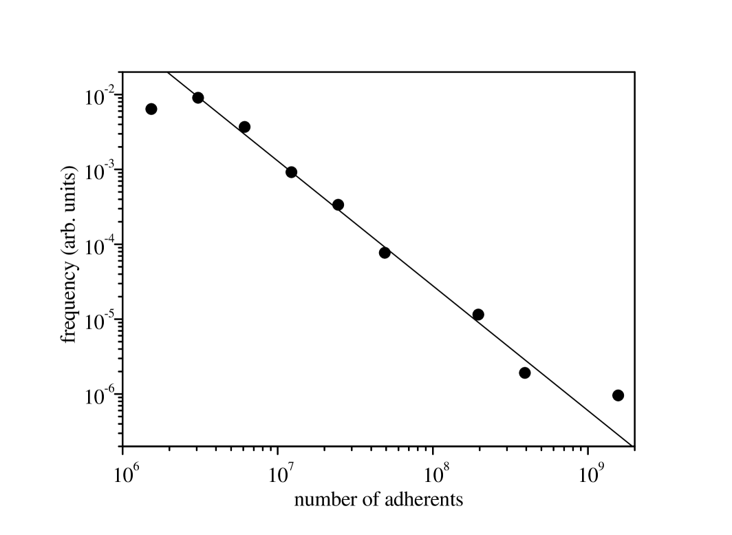
Figure 1: Frequency of religious groups as a function of the number of adherents, in arbitrary units (source: www.adherents.com). The straight line has slope $-5/3\approx-1.67$.

The spatiotemporal dynamics of culture is driven by geographical dissemination of cultural features and by their transmission from old to new generations. Axelrod [3] has proposed a simple model of culture dissemination that captures its basic mechanisms. Cultural features can spread by interaction between individuals, but some preexistent cultural agreement is necessary for such interaction to take place. These mechanisms are able to explain the maintenance of a certain level of cultural diversity. Meanwhile, vertical culture transmission—along the genealogical line, from ancestors to their descendents—is governed by the influence of cultural features in the formation of couples, and by the influence of each parent’s features in determining those of the offspring [4]. Cavalli-Sforza and coworkers have modeled and studied different situations of vertical culture transmission, with special emphasis on the effect of stochastic external agents [5].

An extreme case of vertical transmission of a “cultural” feature, which can be used as a benchmark for models of culture dynamics, is that of family names. An individual’s family name is (in most cases, at least) inherited from the father and, therefore, its possible influence in the formation of the parents’ couple is irrelevant to its transmission. Moreover, creation and mutation of family names are strongly restricted to specific historical periods and places. Most of the time, such changes are extremely rare. The history of family names is, in fact, quite complex [6]. In Europe, for instance, different groups of family names (patronymic-like, toponymic-like, etc.) originated at different times—typically, during the Middle Ages—and mutations became important particularly during the large migration waves within Europe and towards the Americas. New family names appeared also as a consequence of immigration. In spite of this eventful history, current distributions of family names exhibit striking regularities. Figure 2 shows family-name frequencies as a function of the family size—i.e., of the number of individuals bearing a given family name—for the United States and a part of Berlin, in recent times. Both data show a well defined power-law dependence, with an exponent close to $-2$. Analogous data have recently been reported for Japanese family names [7], which exhibit power-law distributions with smaller exponents ($\approx-1.75$).

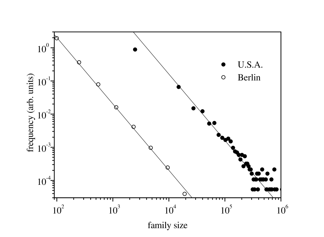
Figure 2: Frequency of family names as a function of the family size, in arbitrary units. The United States data is extrapolated from a sample taken during the 1990 census (source: www.census.gov). The Berlin data corresponds to family names beginning by A, taken from the 1996 phonebook. Family sizes in the Berlin data are multiplied by a factor $10^{2}$ for convenience in displaying. The straight lines have slope $-2$.

In this paper, we consider a model for a growing population where each individual can inherit cultural features from its parents. In particular, we analyze the case of transmission of the family name, and study its distribution as a function of the family size. The parameters relevant to the model are the relative birth rate and the mortality, which control the population growth, and the creation rate of family names. Our preliminary results show that the model satisfactorily reproduces the power laws observed in real data, for wide ranges of the parameters.

2 The model

We introduce in the following a variation of the mechanism proposed by Simon [8] to explain the occurrence of power laws in the frequency distribution of words and city sizes (Zipf’s law [9]), among other instances. In our model, evolution proceeds by discrete steps. At a given step $s$, the $P(s)$ individuals in the population are divided into groups—the families. Within each group, all the individuals share the same family name. At each step, two mechanisms act. (i) A new individual is introduced in the population, representing a birth event. With probability $\alpha$ the newborn is assigned a new family name, not previously present in the population. With the complementary probability, $1-\alpha$, a preexistent individual is chosen at random to become the newborn’s father, and its family name is given to the newborn. Thus, a specific family name is assigned with a probability proportional to the corresponding family size. (ii) An individual is chosen at random from the whole population and, with probability $\mu$, it is eliminated. This represents a death event. Note that if the dead was the only individual with its family name, this specific family name disappears from the population.

The evolution of the population is controled by the parameter $\mu$ which, as we show below, is a direct measure of the mortality rate. The distribution of family names varies due to the effect of family-name creation and mutation, measured by $\alpha$, and of mortality. Since during the evolution the total population $P(s)$ changes, the time interval $\delta t(s)$ to be associated with each evolution step should also change, as $\delta t(s)=1/\nu P(s)$. The frequency $\nu$, whose value is in principle arbitrary, fixes time units. The variation of the population at each step is, on average, $\delta P(s)=1-\mu$. Consequently, the “macrosopic” equation for the time evolution of the population reads

$$\frac{dP}{dt}\approx\frac{\delta P}{\delta t}=\nu(1-\mu)P.$$ (1)

Identifying $\nu$ with the birth rate per individual and unit time, the product $\nu\mu$ is the corresponding mortality rate. In average, thus, the population grows exponentially in time.

Note that, since an individual’s family name is here supposed to be inherited from the father, the model describes the evolution of the male population only. However, the same mechanism can be reinterpreted assuming that the family name is transmitted with the same probability by either parent. In this case, the model encompasses the whole population and no sex distinction occurs. The real situation is in fact intermediate between these two limiting cases. We also stress that in the present model individuals are ageless, in the sense that neither the probability of becoming father of a newborn nor the death probability depend on the individual’s age. As a consequence, the probability $p(m)$ that an individual has $m$ children during its whole life is exponential, $p(m)=\mu(1+\mu)^{-m-1}$. This is to be compared with the Poissonian probability of real, age-structured populations [10].

Below, we consider a class of initial conditions where the population is divided into $N_{0}$ families, with $i_{0}$ individuals in each family. We denote such an initial condition as $(N_{0},i_{0})$. The corresponding initial population is $P(0)=N_{0}i_{0}$.

2.1 Simon’s model: $\mu=0$

Neglecting mortality (that is with $\mu=0$), our system reduces to the model introduced by Simon to explain Zipf’s law [8]. In this case, the evolution of the population is deterministic, $P(s)=P(0)+s$, since exactly one individual is added to the population at each step. Under these conditions, it is possible to write an evolution equation for the average number of families $n_{i}(s)$ with exactly $i$ individuals at step $s$. We have

$$n_{i}(s+1)=n_{i}(s)+\frac{1-\alpha}{P(s)}\left[(i-1)n_{i-1}(s)-in_{i}(s)\right],$$ (2)

for $i>1$, and

$$n_{1}(s+1)=n_{1}(s)+\alpha-\frac{1-\alpha}{P(s)}n_{1}(s).$$ (3)

Simon has shown that, under fairly general conditions, these equations predict a long-time distribution with a power-law decay

$$n_{i}\propto i^{-1-1/(1-\alpha)}$$ (4)

for moderately large values of $i$ ($1\ll i\ll N_{0}+s$). This power-law distribution is to be ascribed to the stochastic multiplicative nature of family growth, which involves a growth probability proportional to the family size. In the limit $\alpha\to 0$ the exponent in Eq. (4) equals $-2$. Note that this limit is relevant to our problem, since the probability of creation or mutation of a family name per individual is expected to be very small. The exponent, in fact, agrees with the empirical data presented in Fig. 2.

We point out that transient effects strongly depend on initial conditions. Figure 3 shows the (normalized) distribution $n_{i}(s)$ calculated from Eqs. (2) and (3) at several evolution stages, for different initial conditions and $\alpha=10^{-3}$. For intermediate values of $i$ the development of the power-law decay with exponent close to $-2$ is apparent in all cases. However, the behaviour of the distribution for larger values of $i$ varies noticeably with the initial condition.

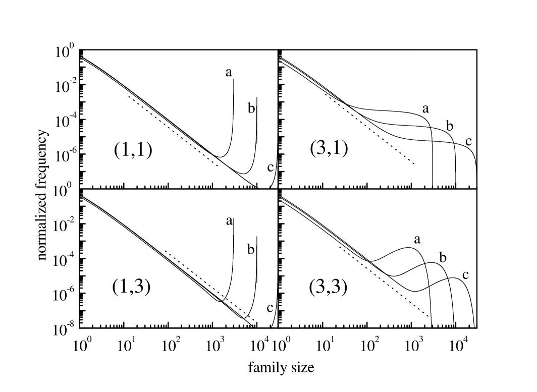
Figure 3: Family-name frequency as a function of the family size, given by Eqs. (2) and (3) with $\alpha=10^{-3}$, at three evolution stages: (a) $s=3\times 10^{3}$, (b) $s=10^{4}$, (c) $s=3\times 10^{4}$. For convenience in displaying, the distributions have been normalized. The numbers in brackets give the initial condition for each case (see text). The dotted straight lines have slope $-2$.

Equations (2) and (3) imply that the total number of family names in the population, given by $N(s)=\sum_{i}n_{i}(s)$, grows in average as $N(s)=N_{0}+\alpha s$. As a function of time, thus, the number of family names increases exponentially, as $N(t)=N_{0}\exp(\alpha t)$, as expected for a population without mortality where family names are created at rate $\alpha$. In contrast, in real populations at present times, the number of family names is known to decrease [6].

2.2 Effects of mortality: $\mu\neq 0$

With $\mu\neq 0$, the growth of the total population $P(s)$ fluctuates stochastically, depending on the occurrence of death events at each evolution step. Consequently, a formulation for the average evolution of $n_{i}(s)$ in terms of a deterministic equation of the form of Eqs. (2) and (3) turns out to be inconsistent. These equation can however be adapted in a way suitable for numerical calculation to the case where the population growth is not deterministic, in the following form. First, for a given value of $P(s)$ at step $s$, the functions in the right-hand side of Eqs. (2) and (3) are applied to $n_{i}(s)$ to obtain intermediate values $n_{i}^{\prime}(s)$. Then, with probability $\mu$, we calculate

$$n_{i}(s+1)=\frac{1}{P(s)+1}\left[(i+1)n_{i+1}^{\prime}(s)-in_{i}^{\prime}(s)\right]$$ (5)

for all $i=1,2,\dots$. Since in this case both birth and death events have taken place, $P(s+1)=P(s)$. With the complementary probability, $1-\mu$, we put $n_{i}(s+1)=n_{i}^{\prime}(s)$ for all $i$, and $P(s+1)=P(s)+1$.

Heuristic arguments—not reproduced here—indicate that, under the conditions used to derive Eq. (4), the above algorithm should give rise to distributions with a well defined power-law decay for moderately large family sizes, of the form

$$n_{i}\propto i^{-1-(1+\mu)/(1+\mu-\alpha)}.$$ (6)

Quite remarkably, in the relevant limit $\alpha\to 0$ the exponent becomes independent of $\mu$, and reduces again to $-2$. For sufficiently low $\alpha$, thus, mortality is not expected to affect the power-law exponent which, as we have seen, is in agreement with empirical data. This has been verified through numerical calculation of $n_{i}(s)$ with the above algorithm, as illustrated in Fig. 4 for the initial condition $(1,1)$ and three values of $\mu$.

The algorithm combining Eqs. (2), (3), and (5) mixes the deterministic average evolution of $n_{i}(s)$ with the stochastic variation of the population, due to random death events. This combination involves, thus, a statistical approximation which must be tested by means of numerical simulations of the fully stochastic model. Results of such simulations, averaged over $10^{4}$ realizations for each value of $\mu$, are shown as dots in Fig. 4. We find very good agreement between both methods.

As for the number of different family names, $N(t)$, we have found that, for moderate values of $\mu$ and at sufficiently long times, it increases exponentially. As expected, the growth rate depends on both $\alpha$ and $\mu$. There is however an initial transient during which the evolution is not exponential and, in fact, $N(t)$ can temporarily decrease. Decay of the number of family names for long times seems to be restricted to very high death probability, $\mu\approx 1$. Note that these are precisely the values expected for $\mu$ in modern developed societies, where birth and death rates are practically identical.

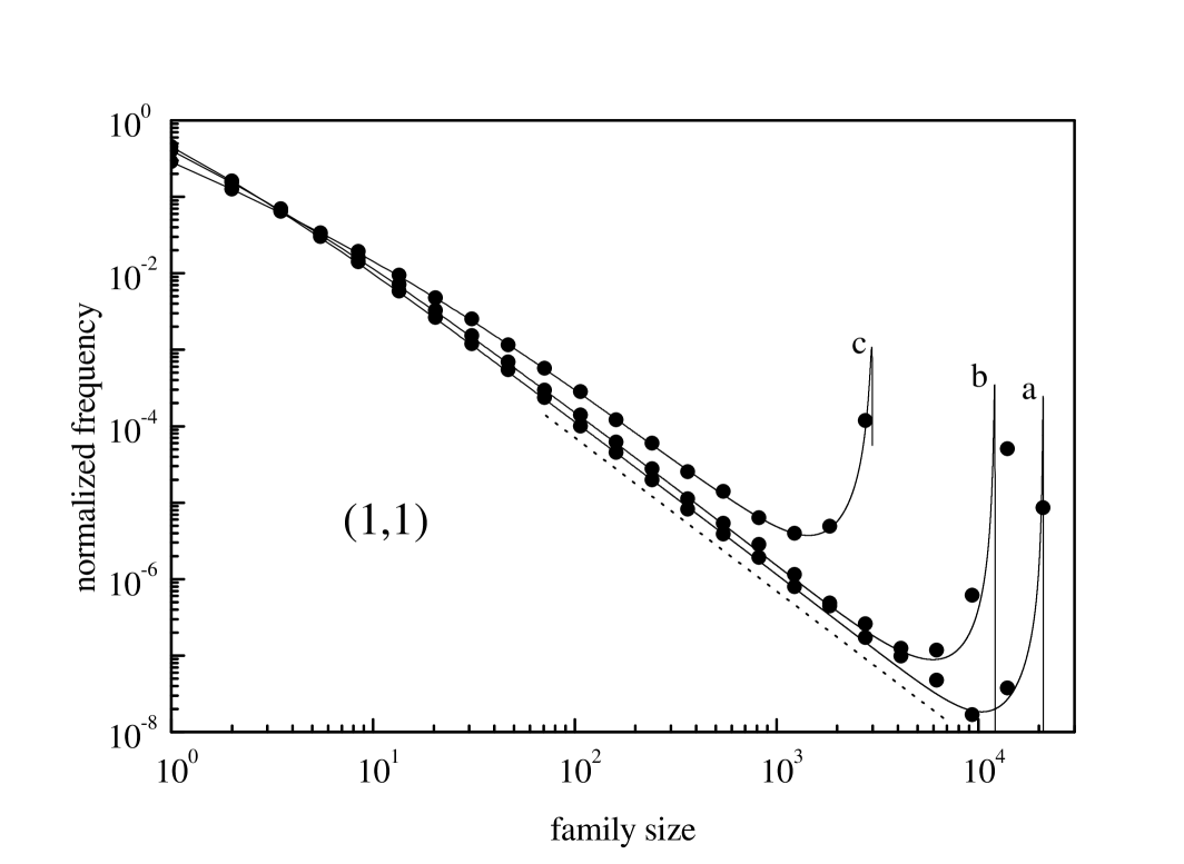
Figure 4: Normalized family-name frequency as a function of the family size calculated from Eqs. (2), (3) and (5) at $s=3\times 10^{4}$, for $\alpha=10^{-3}$ and three values of $\mu$ (a) $\mu=0.3$, (b) $\mu=0.6$, (c) $\mu=0.9$. Dots stand for the results of numerical simulations of the model, averaged over $10^{4}$ realizations. The dotted straight line has slope $-2$.

3 Discussion

The present variant of Simon’s model provides a plausible description of a growing population, as far as the assumption of age-independent fertility and mortality is admitted. The numerical resolution of averaged evolution equations and numerical simulations show that our model successfully reproduces the exponent of power-law distributions observed in the frequency of family names as a function of the family size. Specifically, the exponent close to $-2$ found in empirical data for family names from the United States and Berlin is reproduced in the limit of very small creation and mutation rates and a wide variety of mortality rates.

For other creation and mutation rates, the predicted exponents are, in absolute value, larger than above [cf. Eqs. (4) and (6)]. This contrasts with the exponents found for modern Japanese family names, close to $-1.75$ [7]. We argue that this is an effect of transients which, in this case, are still acting. In fact, most Japanese family names are relatively recent, as they appeared some 120 years ago [7]. Curve (c) in Fig. 4, for instance, shows clearly that transient distributions could be assigned smaller spurious power-law exponents. Note however that a detailed evaluation of transient effects requires a careful identification of initial conditions which, as a result of the complex history of family names, could be a hard task in any real situation.

A quantitative comparison of the predictions of the present model with real data—not presented at this preliminary level—will require considering populations of several million individuals (cf. Fig. 2). Since extensive numerical simulations of systems of such sizes could become computationally too expensive, it will be useful to analyze in detail the scaling properties of our model. In particular, the attention will focus on the dependence of the duration of transients, both in the frequency and in the total number of family names, on the initial population and its distribution in families, as well as on the probabilities $\alpha$ and $\mu$. Considering long-term variations of these probabilities is also in close connection with the comparison of our results with empirical data. In fact, for a modern developed population, in Europe for instance, we can distinguish at least two well differentiated stages. When most European family names appeared, some centuries ago, the total population was increasing more or less steadily. This stage, thus, corresponds to relatively large values of $\alpha$ and moderate values of $\mu$. In modern times, on the contrary, new family names appear at an extremely low rate—in fact, their total number decreases [6]—and the total European population is practically constant, so that $\alpha\approx 0$ and $\mu\approx 1$.

The adaptation of the present model to the study of the evolution of other cultural features requires the addition of two main new ingredients. First, a new parameter must be introduced to define the probability that a given cultural feature is inherited from either parent [4, 5]. Second, it is necessary to specify the effect of that feature in the formation of the parents’ couple, and the mechanism by which couples are effectively formed. This latter process has been classically proposed as an optimization problem [11]. In the frame of our system, it would require a much more realistic approach if any connection with actual populations is to be established.

References

- [1] B. Mandelbrot, Fractals and Scaling in Finance, Springer, New York, 1997.
- [2] J. P. Bouchaud and M. Potters, Theory of Financial Risks: From Statistical Physics to Risk Managment, Cambridge University Press, Cambridge, 2000.
- [3] R. Axelrod, The Complexity of Cooperation, Princeton University Press, 1997.
- [4] L. L. Cavalli-Sforza, M. W. Feldman, K. H. Chen, and S. M. Dornbusch, Science 218 (1982) 19-27.
- [5] L. L. Cavalli-Sforza and M. W. Feldman, Cultural Transmission and Evolution: A Quantitative Approach, Princeton University Press, Princeton, 1981.
- [6] J.-M. Legay and M. Vernay, Pour la Science n. 255 (Jan. 1999) 58-65.
- [7] S. Miyazima, Y. Lee, T. Nagamine, and H. Miyajima, Physica A 278 (2000) 282-288.
- [8] H. A. Simon, Models of Man, Wiley, New York, 1957.
- [9] G. K. Zipf, Human Behavior and the Principle of Least Effort, Addison-Wesley, Cambridge, 1949.
- [10] A. K. Dewdney, Sci. Am. 254 (1986) 12-16.
- [11] M. Dzierzawa and M.-J. Omero, Statistics of stable marriages, cond-mat/0007321, to appear in Physica A.