Abstract

Stationary structures in a classical isotropic two-dimensional continuous Heisenberg ferromagnetic spin system are studied in the framework of the $(2+1)$-dimensional Landau–Lifshitz model. It is established that in the case of $\vec{S}(\vec{r},t)=\vec{S}(\vec{r}-\vec{v}t)$ the Landau–Lifshitz equation is closely related to the Ablowitz–Ladik hierarchy. This relation is used to obtain soliton structures, which are shown to be caused by joint action of nonlinearity and spatial dispersion, contrary to the well-known one-dimensional solitons which exist due to competition of nonlinearity and temporal dispersion. We also present elliptical quasiperiodic stationary solutions of the stationary $(2+1)$-dimensional Landau–Lifshitz equation.

1 Introduction

As it is known, despite of the fact that magnetism is an essentially quantum effect, a wide range of magnetic phenomena can be successfully described in the framework of classical models. One of the most widely used of such models is the one by Landau and Lifshitz, when magnetic is considered in the continuous limit and interaction between magnetic dipoles is taken into account in terms of some effective magnetic field. The simplest case of the Landau–Lifshitz model is the case of the so-called isotropic continuous Heisenberg ferromagnetic spin system, which is governed by the equation

$$\partial_{t}\vec{S}=g\left[\vec{S}\times\Delta\vec{S}\right],\qquad\vec{S}^{2}=1.$$ (1)

Here $\partial_{t}=\partial/\partial t$ and $\Delta$ is the two-dimensional Laplacian, $\Delta=\partial_{xx}+\partial_{yy}$. This equation attaches much attention not only from the viewpoint of its application in the physics of magnetic phenomena, but also from the viewpoint of the theory of integrable nonlinear partial differential equations. It is known that in the $(1+1)$-dimensional case,

$$\partial_{t}\vec{S}=g\left[\vec{S}\times\partial_{xx}\vec{S}\right],$$ (2)

this equation, which has been discussed in a large number of publications (see [1, 2] as well as the books [3, 4, 5] and references therein), can be solved using the inverse scattering transform (IST). Another well studied reduction of (1) is the static two-dimensional case, which may be referred to as $(0+2)$-dimensional one,

$$\left[\vec{S}\times\Delta\vec{S}\right]=0,$$ (3)

(see, e.g., [4]) and which is closely related to the elliptic sine-Gordon model.

The subject of the present paper are the stationary structures of the isotropic two-dimensional classical continuous Heisenberg spin system and we look for solutions of (1) which are of the form

$$\vec{S}=\vec{S}\left(x-v_{x}t,y-v_{y}t\right)$$ (4)

(the so-called Tijon–Wright ansatz with zero frequency [6]).

Of course, this reduction (like any other ansatz) is a necessity, if we want to proceed analytically, and is due to the fact that we cannot at present integrate the original $(2+1)$-dimensional equation.

On the other hand, the stationary structures which are discussed below are of much interest for the physics of magnetism and nonlinear physics in general since they are realization of the so-called dynamical solitons. In physics of magnetic phenomena there exist two types of localized structures. First is the domain walls (kinks) which connect two different ground states and which cannot be destroyed without remagnetising regions of macroscopic sizes (that is why they are called ‘topological solitons’). Another type is solitons, which can be viewed as bound states of a huge number of magnons. The question of their existence and stability, contrary to the case of the topological solitons, is not so trivial. In some sense, they exist due to the presence of some conserved quantities such as number of magnons, total momentum and energy [3]. These are the only physical constants of motion which do not depend on the model we use (as to an infinite number of conservation laws appearing, e.g., in $(1+1)$-dimensional Landau–Lifshitz equation, they seem to be an attribute of the model and do not survive when we move to a more realistic one). The moving stationary structures are the simplest field configurations for which all of the constants are non-zero, i.e. they are the simplest of general (or non-degenerate) ones. Studying these structures one can explicitly see the interaction of the nonlinearity and dispersion which is known to be the core mechanism of creation of localized objects (solitons) not only in magnetic systems but in many other areas of the nonlinear physics.

After substitution (4) equation (1) becomes

$$g\left[\vec{S}\times\Delta\vec{S}\right]+\left(\vec{v},\nabla\vec{S}\right)=0.$$ (5)

Introducing the variables

$$z=\frac{v}{4g}\left[x-v_{x}t+i(y-v_{y}t)\right],\qquad\bar{z}=\frac{v}{4g}\left[x-v_{x}t-i(y-v_{y}t)\right]$$ (6)

where $v=\left|\vec{v}\right|$, we can rewrite it as

$$\left[\vec{S}\times\vec{S}_{z\bar{z}}\right]+\lambda^{2}\vec{S}_{z}+\lambda^{-2}\vec{S}_{\bar{z}}=0$$ (7)

or, equivalently, as

$$\vec{S}_{z\bar{z}}+\left(\vec{S}_{z}\vec{S}_{\bar{z}}\right)\vec{S}+\left[\left(\lambda^{2}\vec{S}_{z}+\lambda^{-2}\vec{S}_{\bar{z}}\right)\times\vec{S}\right]=0$$ (8)

with $\lambda=\exp(i\gamma/2)$, where the angle $\gamma$ is defined by $v_{x}=v\cos\gamma$, $v_{y}=v\sin\gamma$. Equation (7) is known to be integrable (its zero-curvature representation (ZCR) one can find in the paper [6]), and one can tackle it by elaborating the corresponding inverse scattering transform. However, in the present paper we do not discuss this question. Our aim is to establish the relations between the model considered and the other integrable models, which will provide us with a wide range of physically interesting solutions.

For our further purposes it is convenient to rewrite (8) in the matrix form using the correspondence

$$\vec{S}=\left(S_{1},S_{2},S_{3}\right)\rightarrow S=\sum_{a=1}^{3}S_{a}\sigma^{a},$$ (9)

where $\sigma^{a}$ are the Pauli matrices

$$\sigma^{1}=\left(\begin{array}[]{cc}0&1\\ 1&0\end{array}\right),\qquad\sigma^{2}=\left(\begin{array}[]{cc}0&-i\\ i&0\end{array}\right),\qquad\sigma^{3}=\left(\begin{array}[]{cc}1&0\\ 0&-1\end{array}\right).$$ (10)

Equation (8) then can be presented as

$$S_{z\bar{z}}+\frac{1}{2}\left({\rm tr}\,S_{z}S_{\bar{z}}\right)S+\frac{1}{2i}\left[\lambda^{2}S_{z}+\lambda^{-2}S_{\bar{z}}\,,S\right]=0.$$ (11)

Namely this equation is the central object of our investigation.

We will use the following remarkable fact: equation (11) is gauge equivalent to the $O(3,1)$ nonlinear $\sigma$-model [7] in the similar way as, e.g., the $(1+1)$-dimensional classical continuous Heisenberg ferromagnetic spin system (2) is equivalent to the nonlinear Schrödinger equation (see [4, 5]), or the Ishimori magnetic [8] – to the Davey–Stewartson system (see [9]). This equivalence can be briefly described in terms of the IST as follows: some combinations of the Jost functions of the linear problem associated with the $O(3,1)$ $\sigma$-model solve equation (11) (below we shall discuss this question more comprehensively). The fact that model (8), or (11), is related to the $O(3,1)$ nonlinear $\sigma$-model is a generalization of the already known result (see, e.g., [4]) that in the static case equation (3) is gauge equivalent to the elliptic sine-Gordon equation. The $O(3,1)$ $\sigma$-model, as it has been shown in [7], is, in its turn, closely related to the Ablowitz–Ladik hierarchy (ALH) [10]. So we shall establish the direct links between the model considered and the ALH, which is much more well-studied than equations (5), (11) or models [6, 7].

In the present paper we first derive the gauge equivalence between the Heisenberg equation and the ALH (Sections 2, 3) and then use it to obtain soliton solutions (Section 4) and the elliptical quasiperiodic ones (Section 5).

2 The Heisenberg equation and the Ablowitz–Ladik
hierarchy

The method used here, which may be called the ‘embedding into the ALH’ method, has been discussed in [7, 11, 12]. Its main idea is that some equations can be, in some sense, ‘derived’ from the system of differential-difference equations (DDE) belonging to the ALH, which means that any common solution of several equations from the ALH also solves the equation we are dealing with. Relatively to the problem considered this can be briefly outlined as follows.

Consider the system of two equations from the ALH,

$$i\partial_{x}q_{n}=p_{n}\left(q_{n+1}+q_{n-1}\right),$$ (12)

$$\partial_{y}q_{n}=p_{n}\left(q_{n+1}-q_{n-1}\right),$$ (13)

where

$$p_{n}=1-q_{n}r_{n},\qquad r_{n}=-\kappa\bar{q}_{n},\qquad\kappa=\pm 1.$$ (14)

Equation (12) is the well-known discrete nonlinear Schrödinger equation (DNLSE) [13], modified by the substitution $q_{n}\rightarrow q_{n}\exp(2ix)$, while the next one, (13), is the discrete modified KdV equation (DMKdV) [14]. These equations can be rewritten in terms of the complex variables $z=x+iy$, $\bar{z}=x-iy$ as

$$i\partial q_{n}=p_{n}q_{n+1},$$ (15)

$$i\bar{\partial}q_{n}=p_{n}q_{n-1},$$ (16)

where $\partial$ stands for $\partial/\partial z$ and $\bar{\partial}$ for $\partial/\partial\bar{z}$.

It is very important that these equations are compatible, since they belong to the same hierarchy, and the constants of motion that play the role of the Hamiltonians for the flows (12), (13) are in involution. Hence, we can consider them simultaneously, as one system of two equations. It has been shown in [7], and one can easily verify this fact by simple calculations, that, for any fixed $n$, each solution of system (12), (13) also solves the field equations of the $O(3,1)$ nonlinear $\sigma$-model,

$$\partial\bar{\partial}\,q+\frac{(\partial q)(\bar{\partial}q)r}{1-qr}+(1-qr)q=0,\qquad r=-\kappa\bar{q}$$ (17)

and that the quantities $p_{n}$ satisfy the 2D Toda lattice equations

$$\partial\bar{\partial}\,\ln p_{n}=p_{n-1}-2p_{n}+p_{n+1}$$ (18)

(see [11]). Namely this we bear in mind when say that the O(3,1) nonlinear $\sigma$-model and the 2D Toda lattice can be ‘embedded’ into the ALH.

The situation with the Heisenberg spin system is somewhat more difficult. Solution for equation (11) cannot be constructed by means of $q_{n}$’s and $r_{n}$’s only. To do that we have to consider the ZCR for the ALH and to analyze the corresponding linear problems.

The integrable DDEs (15), (16), as well as all equations of the ALH, can be presented as the compatibility condition for the linear system

$$\Psi_{n+1}(\lambda)=U_{n}(\lambda)\Psi_{n}(\lambda),$$ (19)

$$\partial\Psi_{n}(\lambda)=V_{n}(\lambda)\Psi_{n}(\lambda),$$ (20)

$$\bar{\partial}\Psi_{n}(\lambda)=W_{n}(\lambda)\Psi_{n}(\lambda),$$ (21)

where

$$U_{n}=\left(\begin{array}[]{cc}\lambda&r_{n}\\ q_{n}&\lambda^{-1}\end{array}\right)$$ (22)

and the matrices $V_{n}$, $W_{n}$ are given by

$$V_{n}=-i\left(\begin{array}[]{cc}0&\lambda^{-1}r_{n-1}\vspace{1mm}\\ \lambda^{-1}q_{n}&\lambda^{-2}-r_{n-1}q_{n}\end{array}\right),\qquad W_{n}=i\left(\begin{array}[]{cc}\lambda^{2}-q_{n-1}r_{n}&\lambda r_{n}\vspace{1mm}\\ \lambda q_{n-1}&0\end{array}\right).$$ (23)

One can easily see that equations (19), (20) and (19), (21) are compatible only if matrices $U$, $V$ and $W$ satisfy the so-called zero-curvature equations

$$\partial U_{n}=V_{n+1}U_{n}-U_{n}V_{n}$$ (24)

and

$$\bar{\partial}U_{n}=W_{n+1}U_{n}-U_{n}W_{n}$$ (25)

which are equivalent to (15) and (16) correspondingly.

Namely the solutions of the linear problems (19)–(21), $\Psi_{n}$’s, are the key objects of our consideration and the main result of this paper can be formulated as follows: for any $n$, matrices

$$S_{n}=\Psi_{n}^{-1}\sigma^{3}\Psi_{n}$$ (26)

constructed of solutions of the linear problems of the ALH solve the matrix Landau–Lifshitz equation (11).

To derive this result consider matrices $\sigma_{n}^{a}$, $a=1,2,3$ defined by

$$\sigma_{n}^{a}=\sigma_{n}^{a}\left(\lambda;z,\bar{z}\right)=\Psi_{n}^{-1}(\lambda;z,\bar{z})\sigma^{a}\Psi_{n}(\lambda;z,\bar{z}),$$ (27)

where $\sigma^{a}$ is a Pauli matrix (10), and $\Psi_{n}$, recall, is a matrix solution of system (19), (21) (in this notation $S_{n}=\sigma_{n}^{3}$). It follows from (27) and (20), (21) that

$$\partial\sigma^{a}_{n}=\Psi_{n}^{-1}\left[\sigma^{a},V_{n}\right]\Psi_{n},\qquad\bar{\partial}\sigma^{a}_{n}=\Psi_{n}^{-1}\left[\sigma^{a},W_{n}\right]\Psi_{n}.$$ (28)

Using expressions (23) for $V_{n}$ and $W_{n}$ one can find the derivatives of the matrices $S_{n}$ in terms of the matrices $S^{\pm}_{n}$ given by $S^{\pm}_{n}=(1/2)\left(\sigma^{1}_{n}\pm i\sigma^{2}_{n}\right)$ as follows:

$$(i\lambda/2)\;\partial S_{n}=r_{n-1}S^{+}_{n}-q_{n}S^{-}_{n},$$ (29)

$$(i/2\lambda)\;\bar{\partial}S_{n}=-r_{n}S^{+}_{n}+q_{n-1}S^{-}_{n}.$$ (30)

These relations together with analogous expressions for the derivatives $\partial\sigma^{\pm}_{n}$, $\bar{\partial}\sigma^{\pm}_{n}$ and formulae (15), (16), after straightforward calculations, omitted here, lead us to

$$\frac{1}{2}\partial\bar{\partial}S_{n}=\left(q_{n-1}r_{n-1}+q_{n}r_{n}\right)S_{n}+\left(\lambda^{-1}r_{n}-\lambda r_{n-1}\right)S^{+}_{n}+\left(\lambda^{-1}q_{n-1}-\lambda q_{n}\right)S^{-}_{n}.$$ (31)

Noting that

$${\rm tr}\,\partial S_{n}\,\bar{\partial}S_{n}=-4\left(q_{n-1}r_{n-1}+q_{n}r_{n}\right)$$ (32)

and

$$\left[\lambda^{2}\partial S_{n}+\lambda^{-2}\bar{\partial}S_{n}\,,S_{n}\right]=4i\left(\lambda r_{n-1}-\lambda^{-1}r_{n}\right)S_{n}^{+}+4i\left(\lambda q_{n}-\lambda^{-1}q_{n-1}\right)S_{n}^{-}$$ (33)

(both of these formulae follow from (29), (30)) we obtain that for every $n$ the matrix $S_{n}$ solves the equation

$$\partial\bar{\partial}S_{n}+\frac{1}{2}\left({\rm tr}\,\partial S_{n}\bar{\partial}S_{n}\right)S_{n}+\frac{1}{2i}\left[\lambda^{2}\partial S_{n}+\lambda^{-2}\bar{\partial}S_{n}\,,S_{n}\right]=0$$ (34)

which is the main equation of our study, (see (11)). This key result of the present paper can be reformulated in terms of the vector $\vec{S}_{n}$, which corresponds to the matrix $S_{n}$ and which can be presented as

$$\vec{S}_{n}=\left(S_{n1},S_{n2},S_{n3}\right),$$ (35)

where

$$S_{n1}+iS_{n2}=\frac{\Psi_{n}^{(11)}\Psi_{n}^{(21)}}{\Psi_{n}^{(11)}\Psi_{n}^{(22)}-\Psi_{n}^{(12)}\Psi_{n}^{(21)}},\qquad S_{n3}=\frac{\Psi_{n}^{(11)}\Psi_{n}^{(22)}+\Psi_{n}^{(12)}\Psi_{n}^{(21)}}{\Psi_{n}^{(11)}\Psi_{n}^{(22)}-\Psi_{n}^{(12)}\Psi_{n}^{(21)}}$$ (36)

(here $\Psi_{n}^{(ij)}$ are the elements of the matrix $\Psi_{n}$), as follows: for each $n$ the vector $\vec{S}_{n}$ defined by (35), (36) solves equation (8).

Thus we have established the links between equation (11), or (8), describing stationary moving structures in the $(2+1)$-dimensional classical continuous Heisenberg spin system and the ALH. Some more detailed analysis of the gauge equivalence between these models one can find in the next section. However, in this work we are going to focus our attention on ‘practical’ aspects of this relation, so a reader can consider it as an ‘empirical’ fact which can be straightforwardly, and rather easily, verified by the calculations outlined above.

As was mentioned earlier, model (7) is known to be integrable and its zero-curvature representation has already been written out. But, to our knowledge, the corresponding IST has not been elaborated yet, while the ALH is one of the best-studied nonlinear integrable models. Besides, the Heisenberg equation is a vector problem, which somehow complicates inverse scattering analysis, while the ALH is a scalar one. So, to our opinion, the ‘embedding into the ALH’ approach is rather promising and in what follows we demonstrate its usefulness by constructing the soliton and quasiperiodic solutions for the equations considered using the already known solutions for the ALH.

The magnetic energy density, ${\cal W}$,

$${\cal W}\left[\vec{S}\right]=\frac{g}{2}\left(\nabla\vec{S},\nabla\vec{S}\right)$$ (37)

of the field configurations obtained by the embedding into the ALH method can be expressed in terms of the $q_{n}$ and $r_{n}$’s:

$${\cal W}\left[\vec{S}_{n}\right]=-\frac{v^{2}}{4g}\left(q_{n}r_{n}+q_{n-1}r_{n-1}\right).$$ (38)

It can be shown that from the viewpoint of application of solutions of the ALH equations to the description of the vector field $\vec{S}$ one has restrict himself with the case of $\kappa=1$,

$$r_{n}=-\bar{q}_{n},\qquad p_{n}=1+\left|q_{n}\right|^{2}$$ (39)

when the components of the vector $\vec{S}_{n}$ (35) are real (in the opposite case, $\kappa=-1$, the components of $S_{n}$ are complex) and the magnetic energy (38) is positive.

In the next section we will consider the relation between equation (11) and the ALH in the framework of the IST.

3 Gauge equivalence and zero curvature representation

In the previous section we considered the relation between the ALH and the Landau–Lifshitz equation in terms of solutions: we demonstrated how to use solutions of the ALH to obtain ones for the Landau–Lifshitz equation. Now we are going to discuss this question in somewhat more general way. Both the ALH and the Landau–Lifshitz equations are integrable models and it is interesting to describe this correspondence in the language of the IST and to derive links between the auxiliary linear problems which are used to present the integrable models in the zero curvature form (namely this is usually understood when one uses the words ‘gauge equivalence’).

Let us consider again the auxiliary linear problems of the ALH mentioned in Section 2. To our current purposes we do not need the discrete problem (19) and will be dealing with the continuous ones (20), (21). So, we omit now the index $n$ and rewrite (20), (21), (23) as

$$\partial\Psi(\zeta)=V(\zeta)\Psi(\zeta),\qquad\bar{\partial}\Psi(\zeta)=W(\zeta)\Psi(\zeta),$$ (40)

where

$$V(\zeta)=-i\left(\begin{array}[]{cc}0&\zeta^{-1}r_{0}\vspace{1mm}\\ \zeta^{-1}q_{1}&\zeta^{-2}-r_{0}q_{1}\end{array}\right)$$ (41)

and

$$W(\zeta)=i\left(\begin{array}[]{cc}\zeta^{2}-q_{0}r_{1}&\zeta r_{1}\vspace{1mm}\\ \zeta q_{0}&0\end{array}\right)$$ (42)

(we have replaced $q_{n}$, $r_{n}$ with $q_{1}$, $r_{1}$ and $q_{n-1}$, $r_{n-1}$ with $q_{0}$, $r_{0}$). In what follows we denote the spectral parameter by $\zeta$ and use $\lambda$ for its particular value appearing in the definition (27) of the matrix $S$,

$$S=S\left(z,\bar{z}\right)=\Psi^{-1}(\lambda;z,\bar{z})\sigma^{3}\Psi(\lambda;z,\bar{z})$$ (43)

The compatibility (zero-curvature) condition for the system (40)

$$\bar{\partial}V(\zeta)-\partial W(\zeta)+\left[V(\zeta),W(\zeta)\right]=0$$ (44)

leads to the following system of four partial differential equations (PDE) for four unknown functions $q_{1}$, $r_{1}$, $q_{0}$, $r_{0}$:

$$i\partial q_{0}=p_{0}q_{1},$$ (45)

$$i\partial r_{1}=-p_{1}r_{0},$$ (46)

$$i\bar{\partial}q_{1}=p_{1}q_{0},$$ (47)

$$i\bar{\partial}r_{0}=-p_{0}r_{1}.$$ (48)

This system is in some sense intermediate between the DDEs (15), (16) and the PDE (17): both of them can be ‘reconstructed’ from (45)–(48) (we will return to this question below). And namely system (45)–(48) is, strictly speaking, gauge equivalent to the spin field equation we are dealing with.

Now we will derive the ZCR for the stationary $(2+1)$-dimensional Landau–Lifshitz equation from (40) using the gauge transformation by means of the matrix $\Psi(\lambda)$. Introducing the matrix function $\Phi(\zeta)$

$$\Phi(\zeta)=\Psi^{-1}(\lambda)\Psi(\zeta)$$ (49)

one can obtain from (40) that it satisfies the following equations

$$\partial\Phi(\zeta)=V_{L}(\zeta)\Phi(\zeta),\qquad\bar{\partial}\Phi(\zeta)=W_{L}(\zeta)\Phi(\zeta),$$ (50)

where

$$V_{L}(\zeta)=\Psi^{-1}(\lambda)\left[V(\zeta)-V(\lambda)\right]\Psi(\lambda),$$ (51)

$$W_{L}(\zeta)=\Psi^{-1}(\lambda)\left[W(\zeta)-W(\lambda)\right]\Psi(\lambda).$$ (52)

Noting that

$$S_{z}=\Psi^{-1}(\lambda)\left[\sigma^{3},V(\lambda)\right]\Psi(\lambda)=2i\lambda^{-1}\Psi^{-1}(\lambda)\left(\begin{array}[]{cc}0&-r_{0}\\ q_{1}&0\end{array}\right)\Psi(\lambda),$$ (55)

$$S_{\bar{z}}=\Psi^{-1}(\lambda)\left[\sigma^{3},W(\lambda)\right]\Psi(\lambda)=2i\lambda\Psi^{-1}(\lambda)\left(\begin{array}[]{cc}0&r_{1}\\ -q_{0}&0\end{array}\right)\Psi(\lambda)$$ (58)

one can present $V_{L}$ and $W_{L}$ as

$$V_{L}(\zeta)=\frac{i}{2}\left(\zeta^{-2}-\lambda^{-2}\right)\left(S-1\right)+\frac{1}{2}\left(\lambda\zeta^{-1}-1\right)SS_{z},$$ (59)

$$W_{L}(\zeta)=\frac{i}{2}\left(\zeta^{2}-\lambda^{2}\right)\left(S+1\right)+\frac{1}{2}\left(\zeta\lambda^{-1}-1\right)SS_{\bar{z}}.$$ (60)

Using the zero-curvature conditions for equations (50),

$$\bar{\partial}V_{L}-\partial W_{L}+\left[V_{L},W_{L}\right]=0,$$ (61)

and calculating the left-hand-side part of this equation

$$\bar{\partial}V_{L}-\partial W_{L}+\left[V_{L},W_{L}\right]=$$

$$\qquad{}=\frac{1}{2}\left(\frac{\lambda}{\zeta}-\frac{\zeta}{\lambda}\right)\left\{SS_{z\bar{z}}+\frac{1}{2}\left(S_{z}S_{\bar{z}}+S_{\bar{z}}S_{z}\right)+i\lambda^{2}S_{z}+i\lambda^{-2}S_{\bar{z}}\right\}$$ (62)

one can conclude that the matrix $S$ must solve

$$SS_{z\bar{z}}+\frac{1}{2}\left(S_{z}S_{\bar{z}}+S_{\bar{z}}S_{z}\right)+i\lambda^{2}S_{z}+i\lambda^{-2}S_{\bar{z}}=0.$$ (63)

Noting that the anticommutator of traceless $2\times 2$ matrices is proportional to the unit one and that the anticommutator of $S$ and $S_{z}$ or $S_{\bar{z}}$ is zero (which follows from the fact that $\det S=1$, which is another form of the equality $\vec{S}^{2}=1$) one can present this equation in the form (11). Thus the linear problems (50) together with definitions (59) and (60) can be viewed as the ZCR for the main equation of the present paper.

After we have derived the ZCR for (11) we would like to make a few remarks on the application of the inverse scattering technique to non-evolutionary equations as ours. The IST has been originally developed for the Cauchy problems. However, since then much efforts has been made to adjust this method for various boundary value problems. This is a rather difficult task since the latter seem to be more difficult than the former ones. Among successes in this field one should mention results related to the hyperbolic systems such as, e.g, the sine-Gordon equation, the principal chiral field equations etc. For these models the initial value – boundary value problems has been shown to be well stated problems, the existence and uniqueness of the solution has been established and IST-based algorithms to solve, say, the Goursat type boundary problem have been elaborated. One can find discussion of some recent results on boundary problems for the $(1+1)$-dimensional systems on semi-infinite and finite interval, for example in [15].

As to the elliptical systems, similar to the one discussed here, which do not possess characteristics, it is also possible to apply the IST for solving some boundary value problems. Usually it is achieved by breaking the symmetry between the coordinates (which is, of course, not very natural for this kinds of equations), selecting one of them (say, $y$), considering the problem on a half-plane ($y>0$) or on a finite domain (in this case the part of the boundary data plays role of the Cauchy conditions) and performing analysis (i.e. solving the direct and inverse spectral problems) for the auxiliary linear equation corresponding to the complementary coordinate (say, $\Psi_{x}=U\Psi$). One can find examples of such approach in [16] and references therein. However, in this paper we do not discuss the mathematically rigorous formulation of the problem related to (8). We consider here the IST as a method to generate some classes of particular solutions and restrict ourselves to the ones most interesting from the physical viewpoint, solitons and quasiperiodic solutions.

Above we have mapped the $V$-$W$ pair for system (45)–(48) into the $V_{L}$-$W_{L}$ pair for equation (11) by means of the gauge transformation (49),

$$V_{L}(\zeta)=-\Psi^{-1}(\lambda)\partial\Psi(\lambda)+\Psi^{-1}(\lambda)V(\zeta)\Psi(\lambda),$$ (64)

$$W_{L}(\zeta)=-\Psi^{-1}(\lambda)\bar{\partial}\Psi(\lambda)+\Psi^{-1}(\lambda)\widetilde{V}(\zeta)\Psi(\lambda).$$ (65)

Now we are going to derive the inverse transform: from (50) to (40) (i.e. from the $V$-$W$ pair (59), (60) to (41), (42)). The fist step is to diagonalize a solution of the Landau–Lifshitz equation, i.e., to calculate, for given $S$, the matrix $\Psi$ defined by

$$S=\Psi^{-1}\sigma^{3}\Psi.$$ (66)

It is obvious that the $S\rightarrow\Psi$ correspondence is not one-to-one. For any $\Psi$ satisfying (66) the matrix $D\Psi$ with an arbitrary diagonal matrix $D$ will also solve (66). The main point of the Landau–Lifshitz equation $\rightarrow$ ALH transform is to use this arbitrariness to present the matrices $\partial\Psi\cdot\Psi^{-1}$, $\bar{\partial}\Psi\cdot\Psi^{-1}$ in (41), (42) form with $\zeta=\lambda$.

$$\partial\Psi\cdot\Psi^{-1}=V(\lambda)\qquad\mbox{and}\qquad\bar{\partial}\Psi\cdot\Psi^{-1}=W(\lambda).$$ (67)

This step needs some calculations which are presented in the Appendix. Performing then the gauge transform with the found matrix $\Psi$, one can obtain that the transformed $V_{L}$, $W_{L}$ matrices

$$V(\zeta)=\partial\Psi\cdot\Psi^{-1}+\Psi V_{L}(\zeta)\Psi^{-1},$$ (68)

$$W(\zeta)=\bar{\partial}\Psi\cdot\Psi^{-1}+\Psi\widetilde{V}_{L}(\zeta)\Psi^{-1}$$ (69)

are exactly of the form (41), (42) which means that the functions $q_{0}$, $r_{0}$, $q_{1}$, $r_{1}$ (which are defined now in the terms of the matrix $\Psi$ (i.e. in the terms of the matrix $S$) solve the system (45)–(48).

System (45)–(48) that can be rewritten as the DDEs from the ALH. Indeed, starting from the quantities $q_{0}$, $r_{0}$, $q_{1}$, $r_{1}$ one can define the quantities $q_{2}$, $r_{2}$

$$q_{2}=i\frac{\partial q_{1}}{1-q_{1}r_{1}},\qquad r_{2}=-i\frac{\bar{\partial}r_{1}}{1-q_{1}r_{1}}$$ (70)

and demonstrate that they satisfy the following identities:

$$i\bar{\partial}q_{2}=\left(1-q_{2}r_{2}\right)q_{1},\qquad-i\partial r_{2}=\left(1-q_{2}r_{2}\right)r_{1}.$$ (71)

Analogously, the quantities $q_{-1}$, $r_{-1}$,

$$q_{-1}=i\frac{\bar{\partial}q_{0}}{1-q_{0}r_{0}},\qquad r_{-1}=-i\frac{\partial r_{0}}{1-q_{0}r_{0}}$$ (72)

satisfy

$$i\partial q_{-1}=\left(1-q_{-1}r_{-1}\right)q_{0},\qquad-i\bar{\partial}r_{-1}=\left(1-q_{-1}r_{-1}\right)r_{0}.$$ (73)

This procedure can be repeated in both directions

$$\cdots\leftarrow(q_{-1},r_{-1})\leftarrow(q_{0},r_{0},q_{1},r_{1})\rightarrow(q_{2},r_{2})\rightarrow\cdots.$$ (74)

This gives an infinite sequence of $q_{n}$’s, $r_{n}$’s which solve

$$i\partial q_{n}=p_{n}q_{n+1},$$ (75)

$$-i\partial r_{n}=p_{n}r_{n-1}$$ (76)

and

$$i\bar{\partial}q_{n}=p_{n}q_{n-1},$$ (77)

$$-i\bar{\partial}r_{n}=p_{n}r_{n+1},$$ (78)

i.e. the Ablowitz–Ladik DDEs.

To conclude this section we want to discuss the following question. If we start with the ALH, which is a system of DDEs, then the relation between the discrete equations (ALH) and the partial differential Landau–Lifshitz equation is rather obvious: our PDE is a differential consequence of the DDEs. But if we start with the Landau–Lifshitz equation, then what role do the DDEs from the ALH play in the theory of our PDE? In simpler words, what does the subscript $n$ mean in terms of our PDE? The answer is as follows. We have an example of the situation studied by Levi, Benguria [17, 18], Shabat, Yamilov [19] and others: discrete integrable equations (the equations from the ALH in our case) describe sequences of the Bäcklund transformations for some PDEs (the stationary $(2+1)$-dimensional Landau–Lifshitz equation in our case). Indeed, if we have a solution of our equation, $\vec{S}_{1}$, we can derive from it the matrix $\Psi_{1}$ which solves the linear problems for the DNLSE and DMKdV, and hence the quantities $q_{0}$, $r_{0}$, $q_{1}$, $r_{1}$ which solve (45)–(48). Then we can construct the new $\Psi$-matrix $\Psi_{2}=\left(\begin{array}[]{cc}\lambda&r_{1}\\ q_{1}&\lambda^{-1}\end{array}\right)\Psi_{1}$, and the new spin field $\vec{S}_{2}$ which corresponds to the matrix $\Psi_{2}^{-1}\sigma^{3}\Psi_{2}$. This vector field will also solve the Landau–Lifshitz equation. This procedure can be repeated infinitely

$$\cdots\rightarrow\vec{S}_{n}\rightarrow\Psi_{n},q_{n},r_{n}\rightarrow\Psi_{n+1}=U_{n}\Psi_{n}\rightarrow\vec{S}_{n+1}\rightarrow\cdots.$$ (79)

Moreover, it can be performed in other direction

$$\cdots\rightarrow\vec{S}_{n}\rightarrow\Psi_{n},q_{n},r_{n}\rightarrow\Psi_{n-1}=U_{n-1}^{-1}\Psi_{n}\rightarrow\vec{S}_{n-1}\rightarrow\cdots.$$ (80)

Thus we can obtain an infinite number of solutions ( …, $\vec{S}_{-1}$, $\vec{S}_{0}$, $\vec{S}_{1}=\vec{S}$, $\vec{S}_{2}$, …) from one solution $\vec{S}$ and relations between the vectors $\vec{S}_{n}$ with different values of the index $n$ (Bäcklund relations) can be described by the equations which are analogous to (and can be derived from) the DDEs from the ALH.

4 Soliton structures

The discrete nonlinear Schrödinger equation (12) under the condition (39) has been already solved in the pioneering work by Ablowitz and Ladik [13]. As to the solutions of (13), or system (15), (16), they can be obtained by minor modifications of the ones for (12), which is again a manifestation of the fact that all of them belong to the same hierarchy. We will not repeat here the derivation of the IST (one can find the technical details in [13] or, say, in the book [14]) and write down only some final formulae that will be used below.

The $N$-soliton solution of equations (15), (16) can be presented as follows:

$$\bar{q}_{n}(z,\bar{z})=\sum_{j=1}^{N}C_{nj}(z,\bar{z})\xi_{nj}(z,\bar{z}),\qquad\xi_{nj}(z,\bar{z})=\sum_{k=1}^{N}\left[M^{-1}_{n}(z,\bar{z})\right]^{(jk)}\lambda_{k}^{-1}.$$ (81)

The constants $\lambda_{k}$’s are the eigenvalues of the corresponding scattering problem (19) (to be more precise, the discrete spectrum of the scattering problem (19) consists of $N$ pairs of the eigenvalues $(\lambda_{k},-\lambda_{k})$). The functions $C_{nk}(z,\bar{z})$ are given by

$$C_{nk}(z,\bar{z})=C_{k}^{0}\lambda_{k}^{2n}\exp\left\{i\phi_{k}(z,\bar{z})\right\},$$ (82)

where $C_{k}^{0}$’s are arbitrary constants,

$$\phi_{k}(z,\bar{z})=\lambda_{k}^{-2}z+\lambda_{k}^{2}\bar{z},$$ (83)

while the matrix $M$ is given by

$$M=I+\Lambda\bar{A}_{n}\bar{\Lambda}A_{n}.$$ (84)

Here $I$ is the $N\times N$ unit matrix, the overbar stands for the complex conjugation,

$$\Lambda={\rm diag}\,\left(\lambda_{1},\ldots,\lambda_{N}\right)$$ (85)

and $A_{n}$ is the $N\times N$ matrix with the elements

$$A_{n}^{(jk)}(z,\bar{z})=\frac{C_{nk}(z,\bar{z})}{1-\bar{\lambda}_{j}^{2}\lambda_{k}^{2}}$$ (86)

Solution for system (19)–(21) can be presented in the pure soliton case as

$$\Psi_{n}(z,\bar{z})=F_{n}(\lambda;z,\bar{z})\left(\begin{array}[]{cc}\exp(i\lambda^{2}\bar{z})&0\vspace{1mm}\\ 0&\exp(-i\lambda^{-2}z)\end{array}\right),$$ (87)

where $F_{n}(\lambda)$ is the matrix of the following structure:

$$F_{n}(\lambda)=\frac{1}{f_{n}(\infty)}\left(\begin{array}[]{cc}f_{n}(\lambda)&g_{n}(\lambda)\vspace{2mm}\\ -\overline{g_{n}(1/\bar{\lambda})}&\overline{f_{n}(1/\bar{\lambda})}\end{array}\right).$$ (88)

Here

$$f_{n}(\lambda)=1-\lambda^{2}\sum_{j,k=1}^{N}\frac{\bar{C}_{nj}\bar{\lambda}_{j}A_{n}^{(jk)}\xi_{nk}}{1-\lambda^{2}\bar{\lambda}_{j}^{2}},\qquad g_{n}(\lambda)=\lambda\sum_{j=1}^{N}\frac{C_{nj}\xi_{nj}}{\lambda^{2}-\lambda_{j}^{2}}.$$ (89)

The above formulae contain all we need to construct solutions for the Landau–Lifshitz equation (8), or (11). The vertical component of the vector $\vec{S}_{n}$ (see (36)) can be presented, using (87)–(89) and the fact that in our case $\lambda=\exp(i\gamma/2)=1/\bar{\lambda}$ (see remark after (8)), as

$$S_{n3}=1-\frac{2\left|g_{n}(\lambda)\right|^{2}}{f_{n}(\infty)}$$ (90)

while the horizontal components can be written as

$$S_{n1}=S_{n\bot}\cos\varphi_{n},\qquad S_{n2}=S_{n\bot}\sin\varphi_{n},$$ (91)

where

$$S_{n\bot}=\sqrt{1-S_{n3}^{2}},\qquad\varphi_{n}=\arg{f_{n}(\lambda)}-\arg{g_{n}(\lambda)}+\lambda^{-2}z+\lambda^{2}\bar{z}.$$ (92)

The magnetic energy density (37) in this case can be presented, using (38) and the identity $p_{n}=\det F_{n+1}/\det F_{n}$ as

$${\cal W}[\vec{S}_{n}]=\frac{v^{2}}{4g}\left\{\frac{f_{n}(\infty)}{f_{n+1}(\infty)}+\frac{f_{n-1}(\infty)}{f_{n}(\infty)}-2\right\}.$$ (93)

Noting that, for a fixed value of the index $n$, the dependence on $n$ can be taken into account by the redefinition of the constants $C_{k}^{0}$, we may chose $n=0$ and write the final formulae as follows:

$$S_{3}(z,\bar{z})=1-\frac{2\left|g_{0}\left({\rm e}^{i\gamma/2};z,\bar{z}\right)\right|^{2}}{f_{0}(\infty;z,\bar{z})}$$ (94)

and

$$S_{1}(z,\bar{z})=S_{\bot}(z,\bar{z})\cos\varphi(z,\bar{z}),$$ (95)

$$S_{2}(z,\bar{z})=S_{\bot}(z,\bar{z})\sin\varphi(z,\bar{z}),$$ (96)

where

$$S_{\bot}(z,\bar{z})=\sqrt{1-S_{3}^{2}(z,\bar{z})},$$ (97)

$$\varphi(z,\bar{z})=\arg{f_{0}\left({\rm e}^{i\gamma/2};z,\bar{z}\right)}-\arg{g_{0}\left({\rm e}^{i\gamma/2};z,\bar{z}\right)}+{\rm e}^{-i\gamma}z+{\rm e}^{i\gamma}\bar{z}$$ (98)

while the distribution of the magnetic energy of the field configuration given by (94)–(96) can be written as

$${\cal W}=\frac{v^{2}}{4g}\left\{\frac{f_{0}(\infty,z,\bar{z})}{f_{1}(\infty,z,\bar{z})}+\frac{f_{-1}(\infty,z,\bar{z})}{f_{0}(\infty,z,\bar{z})}-2\right\}.$$ (99)

These formulae describe the $N$-soliton solutions of the stationary $(2+1)$-dimensional Landau–Lifshitz equation.

To make clear what kind of solutions we have obtained from the ALH-solitons let us consider in a more detailed way the simplest of the above solutions, namely the one-soliton ones. In this case the quantity $A_{n}(z,\bar{z})=A_{n}^{(11)}(z,\bar{z})$ (see (86)) using the designation

$$\lambda_{1}^{2}=\exp(-2\delta+i\gamma_{1})$$ (100)

can be rewritten as

$$A_{n}(z,\bar{z})=\exp\left\{\chi_{n}+i\psi_{n}\right\},$$ (101)

where

$$\chi_{n}=2\sinh 2\delta\left(\sin\gamma_{1}\cdot{\rm Re}\,z-\cos\gamma_{1}\cdot{\rm Im}\,z\right)-2n\delta+\chi_{*},$$ (102)

$$\psi_{n}=2\cosh 2\delta\left(\cos\gamma_{1}\cdot{\rm Re}\,z+\sin\gamma_{1}\cdot{\rm Im}\,z\right)+n\gamma_{1}+\psi_{*}$$ (103)

and $\chi_{*}$, $\psi_{*}$ are some constants. Setting $n=0$, returning to the real coordinates $x$, $y$ and $t$, and introducing the vectors

$$\vec{k}_{\bot}=\frac{v\sinh 2\delta}{2g}\left(\begin{array}[]{c}\sin\gamma_{1}\\ -\cos\gamma_{1}\end{array}\right),\qquad\vec{k}_{\|}=\frac{v\cosh 2\delta}{2g}\left(\begin{array}[]{cc}\cos\gamma_{1}\\ \sin\gamma_{1}\end{array}\right),$$ (104)

one can rewrite these formulae as

$$A(x,y,t)=\exp\left\{\chi(x,y,t)+i\psi(x,y,t)\right\}$$ (105)

with

$$\chi(x,y,t)=\left(\vec{k}_{\bot},\vec{r}-\vec{v}t\right)+\mbox{const},$$ (106)

$$\psi(x,y,t)=\left(\vec{k}_{\|},\vec{r}-\vec{v}t\right)+\mbox{const}$$ (107)

(here braces stand for the usual scalar product: for $\vec{k}={\mathrm{col}}(k_{x},k_{y})$, $(\vec{k},\vec{r})=k_{x}x+k_{y}y$), from which one can derive the following expressions for the components of the vector $\vec{S}$. The vertical components, $S_{3}$, can be written as

$$S_{3}=1-\frac{2\sinh^{2}2\delta}{\cosh 2\delta-\cos 2\Gamma}\;\frac{1}{\cosh 2\chi+\cosh 2\delta}$$ (108)

where $\Gamma=(\gamma_{1}-\gamma)/2$, or, equivalently, as

$$S_{3}=\cos\theta$$ (109)

with the angle $\theta$ being given by

$$\tan\frac{\theta}{2}=\left[\left(\frac{\sin\Gamma}{\sinh\delta}\cosh\chi\right)^{2}+\left(\frac{\cos\Gamma}{\cosh\delta}\sinh\chi\right)^{2}\right]^{-1/2}.$$ (110)

The horizontal components $S_{1,2}$ can be presented as

$$\left(\begin{array}[]{c}S_{1}\\ S_{2}\end{array}\right)=\sin\theta\left(\begin{array}[]{c}\cos\varphi\\ \sin\varphi\end{array}\right)$$ (111)

with

$$\varphi(x,y,t)=\hat{\varphi}(x,y,t)+\left(\vec{k}_{0}-\vec{k}_{\|},\vec{r}-\vec{v}t\right)+\mbox{const}.$$ (112)

Here, the vector $\vec{k}_{0}$,

$$\vec{k}_{0}=\frac{v}{2g}\left(\begin{array}[]{c}\cos\gamma\\ \sin\gamma\end{array}\right),$$ (113)

is parallel to the velocity vector, $\vec{k}_{0}=\vec{v}/2g$, and is related to $\vec{k}_{\bot}$, $\vec{k}_{\|}$ by $\vec{k}_{0}^{2}=\vec{k}_{\|}^{2}-\vec{k}_{\bot}^{2}$. The function $\hat{\varphi}$ is given by

$$\hat{\varphi}=\arctan\left(\tanh\delta\,\cot\Gamma\,\tanh\chi\right).$$ (114)

The magnetic energy of this field configuration can be written as

$${\cal W}=4gk_{\bot}^{2}\frac{1+\cosh 2\delta\,\cosh 2\chi}{\left(\cosh 2\chi+\cosh 2\delta\right)^{2}},$$ (115)

where $k_{\bot}$ stands for $|\vec{k}_{\bot}|$.

It can be shown that ${\cal W}$ (115) is a second-order polynomial in $S_{3}$:

$${\cal W}=-g\vec{k}_{\|}^{2}S_{3}^{2}+\left(\vec{v},\vec{k}_{\|}\right)S_{3}+{\cal W}_{0},$$ (116)

where ${\cal W}_{0}$ is some constant. The linear energy density, ${\cal W}_{\rm lin}$,

$${\cal W}_{\rm lin}=\int_{-\infty}^{\infty}dx_{\bot}{\cal W}(x,y,t),\qquad x_{\bot}=\left(\frac{\vec{k}_{\bot}}{k_{\bot}}\,,\vec{r}\right)$$ (117)

can be easily shown to be

$${\cal W}_{\rm lin}=4gk_{\bot}.$$ (118)

To simplify the following analysis let us consider the case when the velocity vector is directed along the $x$-axis ($\gamma=0$, $\lambda=1$). This does not lead to loss of generality because solutions corresponding the arbitrary vector $\vec{v}=(v\cos\gamma,v\sin\gamma)$ can be obtained from the ones presented below by the substitution $x\rightarrow x\cos\gamma+y\sin\gamma$, $y\rightarrow y\cos\gamma-x\sin\gamma$. It can be easily seen that formulae (108)–(112) in the limiting cases $\gamma_{1}=\pi/2$ and $\gamma_{1}=0$ describe essentially different field structures. In the case $\gamma_{1}=\pi/2$ ($\Gamma=\pi/4$)

$$\chi=\chi(x-vt)=k_{\bot}\left(x-x_{*}-vt\right)$$ (119)

with an arbitrary constant $x_{*}$, and both $S_{3}$ and ${\cal W}$ depend on $x-vt$ only,

$$\theta=\theta(x-vt)=2\arctan\left(\frac{\sinh 2\delta}{\left[\cosh^{2}(\chi+\delta)+\cosh^{2}(\chi-\delta)\right]^{1/2}}\right),$$ (120)

$${\cal W}={\cal W}(x-vt)=gk_{\|}^{2}\sin^{2}\theta(x-vt)$$ (121)

while $\varphi$ can be written as

$$\varphi(x,y,t)=\hat{\varphi}(x-vt)+k_{0}(x-vt)+k_{\|}y+\mbox{const},$$ (122)

where

$$\hat{\varphi}(x)=\arctan\left(\tanh\delta\,\tanh k_{\bot}(x-x_{*})\right).$$ (123)

So, this solution describes a localized structure, moving in the $x$-direction, which is phase modulated in the transversal direction ($y$-direction), and it may be termed ‘quasi one-dimensional soliton’ (see Fig. 1).

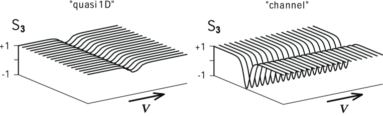
Figure 1: Limiting cases of the one-soliton solutions (schematically) corresponding to $\Gamma=\pi/4$ and $\Gamma=0$.

The soliton obtained above is essentially two-dimensional structure and despite apparent similarity it cannot be reduced to its one-dimensional analogue. Indeed, in the one-dimensional case soliton solutions of equation (2) possess the following form:

$$\theta=\theta\left(\frac{x-vt}{L(\Omega)}\right),\qquad\varphi=\Omega t+\hat{\varphi}\left(\frac{x-vt}{L(\Omega)}\right),$$ (124)

and one can say that such solitons exist due to the temporal phase modulation of the whole medium, which manifests itself in the fact that $L(\Omega)\propto\Omega^{-1/2}$, i.e., soliton vanishes with $\Omega$ going to zero. In other words, these one-dimensional soliton structures do not exist in absence of the phase modulation $\Omega t$. In our case, existence of solitons is due to the spatial phase modulation (in $y$-direction), which manifests itself in the fact that the magnetic energy density is proportional to $\vec{k}_{\|}^{2}$. In other words, solitons we have obtained differ from their one-dimensional analogues in the physical mechanism lying in their background: they are caused by the competition between the spatial dispersion and nonlinearity while in the one-dimensional case solitons are caused by the competition between the temporal dispersion and nonlinearity.

In the opposite case, $\gamma_{1}=0$ ($\Gamma=0$),

$$\theta=\theta(y)=2\arctan\frac{\cosh\delta}{\sinh k_{\bot}(y-y_{*})},$$ (125)

i.e. $S_{3}$, which can be written as

$$S_{3}=S_{3}(y)=\frac{\sinh^{2}k_{\bot}\left(y-y_{*}\right)-\cosh^{2}\left(\delta_{1}/2\right)}{\sinh^{2}k_{\bot}\left(y-y_{*}\right)+\cosh^{2}\left(\delta_{1}/2\right)},$$ (126)

depends on $y$ only (and, what is essential, does not depend on time), while the horizontal components are rotating with constant frequency:

$$\varphi=\varphi(x-vt)=\kappa_{x}(x-vt),$$ (127)

where

$$\kappa_{x}=k_{\|}-k_{0}$$ (128)

and $k_{a}$, remind, stands for $|\vec{k}_{a}|$.

This solution describes the spin wave localized in the $2k_{\bot}^{-1}$-neighborhood of the line $y=y_{*}$ (this field distribution, which is depicted schematically in the Fig. 1, may be termed ‘channel’). The magnetic energy of the ‘channel’ field configuration does not depend on time, ${\cal W}={\cal W}(y)$, hence it can be considered as almost static, in the sense that we have no energy transport in this case. Similar structures have been found by A S Kovalev [20].

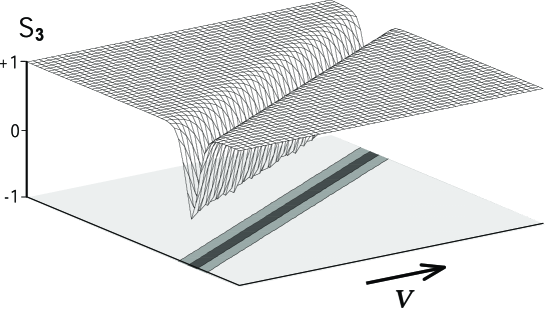
Figure 2: One-soliton solution for $\lambda=1$ and $\lambda_{1}=0.8\exp(i\pi/12)$

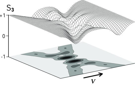
Figure 3: Two-soliton solution for $\lambda=1$ and $\lambda_{1}=\bar{\lambda}_{2}=0.8\exp(i\pi/12)$

The character of the soliton field structure in the general case $0<\gamma_{1}<\pi/2$ can be seen from the Fig. 2. The many-soliton structures in the general case can be viewed as consisting of several intersecting solitons. One can find typical two-soliton spin distribution in the Fig. 3.

5 Quasiperiodic structures

The ALH in the quasiperiodic case is less studied than in the soliton one. Several authors have discussed the quasiperiodic solutions (QPS) for the discrete nonlinear Schrödinger and the discrete modified Korteveg-de Vries equations (see, e.g., [22, 21]), but their results are not enough to construct the corresponding solutions for the Heisenberg equation using the ‘embedding into the ALH’ method. What we need and what is absent in the papers [22, 21] is a solution of the auxiliary system (19)–(21) which in the quasiperiodic case is known as the Baker–Akhiezer function. Later this question was solved in [23] (see also [24]). However, these results, describing general finite-genus solutions, are rather cumbersome, so here we restrict ourselves only to the elliptic solutions, which are the simplest QPS.

The elliptic solutions for system (15), (16) possess the following structure:

$$q_{n}=q_{*}\varepsilon^{n}{\rm e}^{i\phi}\frac{\vartheta_{1}(\zeta_{n}+\alpha)}{\vartheta_{1}(\zeta_{n})},\qquad r_{n}=r_{*}\varepsilon^{-n}{\rm e}^{-i\phi}\frac{\vartheta_{1}(\zeta_{n}-\alpha)}{\vartheta_{1}(\zeta_{n})},$$ (129)

where $\vartheta_{1}$ is one of the elliptic theta-functions (see, e.g. [25]), the phase $\phi$ is some linear function of the coordinates $z$ and $\bar{z}$ (it will be specified below),

$$\zeta_{n}=\frac{z}{L}+\frac{\bar{z}}{\tilde{L}}+n\beta+\mbox{const}$$ (130)

and the constants $q_{*}$, $r_{*}$ are related by

$$q_{*}r_{*}=-\frac{\vartheta_{1}^{2}(\beta)}{\vartheta_{1}(\alpha+\beta)\vartheta_{1}(\alpha-\beta)}.$$ (131)

The quantities $p_{n}$’s can be presented as

$$p_{n}=\frac{\vartheta_{1}^{2}(\alpha)}{\vartheta_{1}(\alpha+\beta)\vartheta_{1}(\alpha-\beta)}\frac{\vartheta_{1}(\zeta_{n}+\beta)\vartheta_{1}(\zeta_{n}-\beta)}{\vartheta_{1}^{2}(\zeta_{n})}$$ (132)

which follows from expressions (129) and the identity

$$\vartheta_{1}^{2}(x)\vartheta_{1}(y+z)\vartheta_{1}(y-z)+\vartheta_{1}^{2}(y)\vartheta_{1}(z+x)\vartheta_{1}(z-x)$$

$$\qquad{}+\vartheta_{1}^{2}(z)\vartheta_{1}(x+y)\vartheta_{1}(x-y)=0.$$ (133)

This identity is the Fay’s formulae [26] for the elliptic functions. It can be used to calculate the derivatives of the $\vartheta$-functions. Differentiating (133) with respect to $z$ and putting $z=y$ one can obtain for the logarithmic derivative $\psi$,

$$\psi(\zeta)=\frac{{\rm d}}{{\rm d}\zeta}\ln\vartheta_{1}(\zeta),$$ (134)

the relation:

$$\psi(\zeta+x)-\psi(\zeta-x)=2\psi(x)-\frac{\vartheta_{1}^{\prime}(0)\vartheta_{1}(2x)}{\vartheta_{1}^{2}(x)}\frac{\vartheta_{1}^{2}(\zeta)}{\vartheta_{1}(\zeta+x)\vartheta_{1}(\zeta-x)}.$$ (135)

Using the latter one can obtain that functions (129) satisfy equations (15), (16) provided the scales $L$ and $\tilde{L}$ are chosen as

$$L=i\vartheta_{1}^{\prime}(0)\frac{\vartheta_{1}(\alpha-\beta)}{\vartheta_{1}(\alpha)\vartheta_{1}(\beta)}\varepsilon^{-1},\qquad\tilde{L}=-i\vartheta_{1}^{\prime}(0)\frac{\vartheta_{1}(\alpha+\beta)}{\vartheta_{1}(\alpha)\vartheta_{1}(\beta)}\varepsilon,$$ (136)

and the phase $\phi$ is given by

$$\phi=-i\left[\psi(\beta)-\psi(\beta+\alpha)\right]\frac{z}{L}+i\left[\psi(\beta)-\psi(\beta-\alpha)\right]\frac{\bar{z}}{\tilde{L}}+\mbox{const}.$$ (137)

The Baker–Akhiezer function of our problem (i.e. the quasiperiodic solution for system (20)), (21) can be written as a matrix with the elements

$$\Psi^{(11)}_{n}(\lambda)=A_{1}\mu_{1}^{n}\frac{\theta(\zeta_{n}+\eta)}{\theta(\zeta_{n}-\beta)}\exp(i\Phi_{1}),$$ (138)

$$\Psi^{(21)}_{n}(\lambda)=-A_{1}\mu_{1}^{n}\lambda^{-1}q_{n-1}\frac{\theta(\alpha-\beta)\theta(\eta)}{\theta(\beta)\theta(\eta+\alpha)}\frac{\theta(\zeta_{n}+\eta+\alpha)}{\theta(\zeta_{n}+\alpha-\beta)}\exp(i\Phi_{1}),$$ (139)

$$\Psi^{(12)}_{n}(\lambda)=A_{2}\mu_{2}^{n}\lambda r_{n-1}\frac{\theta(\alpha+\beta)\theta(\eta+\beta)}{\theta(\beta)\theta(\eta+\alpha+\beta)}\frac{\theta(\zeta_{n}-\eta-\alpha-\beta)}{\theta(\zeta_{n}-\alpha-\beta)}\exp(i\Phi_{2}),$$ (140)

$$\Psi^{(22)}_{n}(\lambda)=A_{2}\mu_{2}^{n}\frac{\theta(\zeta_{n}-\eta-\beta)}{\theta(\zeta_{n}-\beta)}\exp(i\Phi_{2}).$$ (141)

Here $A_{1,2}$ are arbitrary constants which are of no importance for our further consideration. The phases $\Phi_{1,2}$ are the linear functions of the coordinates,

$$\Phi_{1}=\left[\psi(\eta+\alpha+\beta)-\psi(\alpha)\right]\frac{iz}{L}+\left[\psi(\eta+\beta)+\psi(\alpha)-\psi(\alpha-\beta)-\psi(\beta)\right]\frac{i\bar{z}}{\tilde{L}},$$ (142)

$$\Phi_{2}=\left[-\psi(\eta)+\psi(\alpha+\beta)-\psi(\alpha)-\psi(\beta)\right]\frac{iz}{L}+\left[-\psi(\eta+\alpha)+\psi(\alpha)\right]\frac{i\bar{z}}{\tilde{L}},$$ (143)

the quantities $\mu_{1,2}$ are given by

$$\mu_{1}=\lambda\frac{\theta(\alpha)\theta(\eta+\alpha)}{\theta(\alpha-\beta)\theta(\eta+\alpha+\beta)},\qquad\mu_{2}=\lambda^{-1}\frac{\theta(\alpha)\theta(\eta+\alpha+\beta)}{\theta(\alpha+\beta)\theta(\eta+\alpha)}$$ (144)

and $\eta$ can be determined as a solution of the equation

$$\frac{\vartheta_{1}(\alpha-\beta)}{\vartheta_{1}(\alpha+\beta)}\,\frac{\vartheta_{1}(\eta)\vartheta_{1}(\eta+\alpha+\beta)}{\vartheta_{1}(\eta+\alpha)\vartheta_{1}(\eta+\beta)}=\varepsilon\lambda^{2}$$ (145)

(in the framework of the general theory, $\eta$ can be considered as the point of the Riemann surface that corresponds to the point $\varepsilon\lambda^{2}$ of the complex plane).

These formulae (we do not present here the corresponding derivation procedure) can be verified straightforwardly using (135) and (133). They provide all necessary to construct the elliptic solutions for the Heisenberg equation (11). Using (36), (109) and (111), and omitting the $n$-dependence one can obtain

$$\tan^{2}\frac{\theta}{2}=-\frac{\vartheta_{1}(\eta)\vartheta_{1}(\eta+\beta)}{\vartheta_{1}(\eta+\alpha)\vartheta_{1}(\eta+\alpha+\beta)}\frac{\vartheta_{1}(\zeta+\eta+\alpha)\vartheta_{1}(\zeta-\eta-\alpha-\beta)}{\vartheta_{1}(\zeta+\eta)\vartheta_{1}(\zeta-\eta-\beta)}$$ (146)

and

$$\exp\left\{2i\varphi\right\}=\frac{\vartheta_{1}(\zeta+\eta)\vartheta_{1}(\zeta+\eta+\alpha)}{\vartheta_{1}(\zeta-\eta-\beta)\vartheta_{1}(\zeta-\eta-\alpha-\beta)}\exp\left\{2i\Phi\right\},$$ (147)

where

$$\Phi=\Phi_{1}-\Phi_{2}+\phi.$$ (148)

The last two formulae can be rewritten as

$$\varphi=\widehat{\varphi}(\zeta)-\widehat{\varphi}^{{}^{\prime}}(0)\zeta-\left(\vec{\kappa}_{\|},\vec{r}-\vec{v}t\right),$$ (149)

$$\widehat{\varphi}(\zeta)=\frac{1}{2i}\ln\frac{\vartheta_{1}(\zeta+\eta)\vartheta_{1}(\zeta+\eta+\alpha)}{\vartheta_{1}(\zeta-\eta-\beta)\vartheta_{1}(\zeta-\eta-\alpha-\beta)}.$$ (150)

Here the vector $\vec{\kappa}_{\|}$ is given by

$$\vec{\kappa}_{\|}=\kappa_{\|}\left(\begin{array}[]{c}\cos\gamma_{1}\\ \sin\gamma_{1}\end{array}\right)$$ (151)

with

$$\kappa_{\|}^{2}=\frac{v^{2}}{4g^{2}}\,\frac{\vartheta_{1}^{4}(\alpha)\vartheta_{1}^{4}(\beta)\vartheta_{1}^{2}(2\eta+\alpha+\beta)}{\vartheta_{1}^{2}(\eta)\vartheta_{1}^{2}(\eta+\alpha)\vartheta_{1}^{2}(\eta+\beta)\vartheta_{1}^{2}(\eta+\alpha+\beta)\vartheta_{1}(\alpha+\beta)\vartheta_{1}(\alpha-\beta)}$$ (152)

and the angle $\gamma_{1}$ is defined by

$${\rm e}^{2i\gamma_{1}}=\frac{1}{\varepsilon^{2}}\,\frac{\vartheta_{1}(\alpha-\beta)}{\vartheta_{1}(\alpha+\beta)}.$$ (153)

The magnetic energy density ${\cal W}$ (37) of the above field configuration is, as in the one-soliton case, a second-order polynomial in $S_{3}$:

$${\cal W}=-g\vec{\kappa}_{\|}^{2}S_{3}^{2}+\left(\vec{v},\vec{\kappa}_{\|}\right)S_{3}+{\cal W}_{0},$$ (154)

where ${\cal W}_{0}$ is some constant. The last formula again illustrates the importance of the transversal modulation (space dispersion) for the existence of our nonlinear structures.

It should be noted that to ensure reality of all physical quantities, such as $S_{i}$, ${\cal W}$ one has to impose some restrictions on the parameters $\alpha$, $\beta$ and $\eta$ (or $\varepsilon$) which appear in the above expressions. We cannot at present formulate these restrictions in their general form, but will show below how these parameters should be chosen in some particular case, which is a generalization of the pure soliton one, in the sense that the one-soliton solutions obtained in Section 4 are some limiting cases ot the elliptical ones discussed below.

Thus, in what follows we restrict ourselves with the case of

$$\alpha=\frac{\tau}{2},$$ (155)

where $\tau$ is the complex half-period of the $\vartheta_{1}$-function (see [25]). It can be shown that in this case both the components of the vector $\vec{S}$ and the energy ${\cal W}$ will be real if we choose

$$\zeta=\frac{1+\beta}{2}-i\hat{\zeta},\qquad\eta=\hat{\eta}-\frac{\beta}{2},\qquad\beta=2i\hat{\beta},$$ (156)

where hats indicate that correspondent quantities are real. In what follows we use together with the theta-functions also the Jacobian elliptical functions ${\rm sn}$, ${\rm cn}$ and ${\rm dn}$,

$${\rm sn}\,u={\rm sn}\,(u,k)=\frac{\vartheta_{3}(0)}{\vartheta_{2}(0)}\,\frac{\vartheta_{1}(u/2K)}{\vartheta_{0}(u/2K)}$$ (157)

with

$$k=\frac{\vartheta_{2}^{2}(0)}{\vartheta_{3}^{2}(0)},\qquad K=\frac{\pi}{2}\vartheta_{3}^{2}(0)$$ (158)

(the definition of $\vartheta_{2,3}$ and analogous formulae for ${\rm cn}\,u$ and ${\rm dn}\,u$ one can find, e.g., in [25]). The ‘coordinate’ $\hat{\zeta}$ can be written now as

$$\hat{\zeta}=\frac{1}{\pi}\left(\vec{k}_{\bot},\vec{r}-\vec{v}t\right),$$ (159)

where

$$\vec{k}_{\bot}=\frac{v}{2g}\,\frac{\pi}{2K}\,\frac{{\rm sn}\,4iK\hat{\beta}}{i}\left(\begin{array}[]{c}\sin\gamma_{1}\\ -\cos\gamma_{1}\end{array}\right).$$ (160)

The expressions for $\theta$ and $\varphi$ (146) and (149), (150) can be presented as

$$\tan^{2}\frac{\theta}{2}=\left|{\rm sn}\left(2K\hat{\eta}+2iK\hat{\beta}\right)\,\frac{{\rm dn}\left(2K\hat{\eta}+2iK\hat{\zeta}\right)}{{\rm cn}\left(2K\hat{\eta}+2iK\hat{\zeta}\right)}\right|^{2}$$ (161)

and

$$\varphi=\left(\vec{\kappa}_{0}-\vec{\kappa}_{\|},\vec{r}-\vec{v}t\right)+{\rm arg}\,\left[\vartheta_{2}(\hat{\eta}-i\hat{\zeta})\vartheta_{3}(\hat{\eta}-i\hat{\zeta})\right].$$ (162)

The vector $\vec{\kappa}_{0}$ is given by

$$\vec{\kappa}_{0}=\frac{2}{\pi}\left[{\rm Re}\,\psi_{0}\left(\hat{\eta}+i\hat{\beta}\right)\right]\vec{k}_{\bot},$$ (163)

where

$$\psi_{0}(z)=\psi(z)-K\frac{{\rm cn}\,2Kz\;{\rm dn}\,2Kz}{{\rm sn}\,2Kz}=\psi(z)-\frac{\pi}{2}\vartheta_{0}^{2}(0)\frac{\vartheta_{2}(z)\vartheta_{3}(z)}{\vartheta_{1}(z)\vartheta_{0}(z)}$$ (164)

while the vector $\vec{\kappa}_{\|}$ is given by (151) with

$$\kappa_{\|}=i\,\frac{v}{g}\,\frac{{\rm sn}\,4iK\hat{\beta}}{{\rm sn}\,4K\hat{\eta}}\sin 2\Gamma$$ (165)

and $\Gamma=(\gamma_{1}-\gamma)/2$ is related to $\hat{\beta}$ and $\hat{\eta}$ by

$${\rm e}^{2i\Gamma}=\frac{{\rm sn}\,2K(\hat{\eta}+i\hat{\beta})}{{\rm sn}\,2K(\hat{\eta}-i\hat{\beta})}.$$ (166)

It is straightforward to show that the limiting case of the elliptic quasiperiodic solutions presented above is solitons obtained in Section 4. Indeed, with the parameter $k$ (158) going to zero (which corresponds to $\tau\rightarrow i\infty$), the elliptic functions sn, cn and dn become sin, cos and 1 correspondingly. Noting that $K(k=0)=\pi/2$ and identifying $\pi\hat{\beta}$ with $\delta$ (which implies $\pi\hat{\zeta}\rightarrow\chi$) one can transform (161) and (162) to formulae (110) and (112) describing solutions of the Landau–Lifshitz equation in the one-soliton case.

6 Conclusion

To conclude, we want to summarize the main results and to outline some perspectives of the studies discussed in this paper. From the mathematical point of view, our main result is the established relation between the Landau–Lifshitz equation (in the case $\vec{S}(\vec{r},t)=\vec{S}(\vec{r}-\vec{v}t)$) and the ALH. And though we cannot at present provide general explanation of what makes such apparently different models be so closely connected, we hope that the results presented in Sections 4, 5 are rather convincing arguments in favour of the fact that this relation is useful, at least from the practical standpoint, as a tool for generating of a large number of solutions. On the other hand, this work presents 2D stationary structures of the isotropic continuous Heisenberg ferromagnetic spin system which have not been, to our knowledge, discussed in the literature and which seem to be interesting for the physics of magnetic phenomena. It should be noted that we have obtained our results in the framework of the classical model, and one of the most important questions that should be solved now, from the viewpoint of applications to magnetism, is to develop quantum, or at least semi-classical, theory of such structures. Another question we want to mention here is the following one. It is a widely known fact that solitons appear as a result of joint action of nonlinearity and some other mechanisms, such as dispersion. In our consideration we have neglected the temporal dispersion (temporal modulation), and its role has been played by the spatial one. So, it is interesting to take into account both temporal and spatial dispersions, because the competition of different mechanisms in nonlinear regime can lead to nontrivial results. These and some other related questions may be the subject of further investigations.

Acknowledgements

This work was partly carried out during the authors’ stay at the Abdus Salam International Centre for Theoretical Physics which is gratefully acknowledged for its kind hospitality and was partly supported by the Ministerio de Educación, Cultura y Deporte of Spain under grant SAB2000-0256. We are grateful to A S Kovalev for useful and stimulating discussions.

Appendix

The aim of this section is to derive the matrix $\Psi$ related to the solution of equation (11) $S$ by

$$S=\Psi^{-1}\sigma^{3}\Psi$$ (A.1)

such that the matrices $V$, $W$

$$V=\partial\Psi\cdot\Psi^{-1},\qquad W=\bar{\partial}\Psi\cdot\Psi^{-1}$$ (A.2)

have the structure of the ALH matrices (41), (42). The diagonalization (A.1) of a given matrix $S$ is not unique. Suppose we have found a matrix $F$ satisfying

$$S=F^{-1}\sigma^{3}F.$$ (A.3)

Then any matrix

$$\Psi=DF$$ (A.4)

with an arbitrary diagonal matrix $D=\mathrm{diag}\left(D_{11},D_{22}\right)$ satisfies (A.1). Hence, to solve our problem we can start from any solution of (A.3), for example from one given by

$$F=1+\sigma^{3}S$$ (A.5)

(one can verify by simple calculations that this is indeed a solution of (A.3)) and then to construct the diagonal matrix $D$ such that the matrices

$$V=\partial\Psi\cdot\Psi^{-1}=\partial D\cdot D^{-1}+D\,\partial F\cdot F^{-1}\,D^{-1},$$ (A.6)

$$W=\bar{\partial}\Psi\cdot\Psi^{-1}=\bar{\partial}D\cdot D^{-1}+D\,\bar{\partial}F\cdot F^{-1}\,D^{-1}$$ (A.7)

possess the properties we need.

To simplify the following formulae let us introduce the designation $a$, $b$ and $c$ for the elements of the matrix $S$,

$$S=\left(\begin{array}[]{cc}a&b\\ c&-a\end{array}\right).$$ (A.8)

The main equation of this paper (A.3) can be rewritten now as a system

$$a_{z\bar{z}}+aX+\frac{i}{2}\left(bc^{\prime}-b^{\prime}c\right)=0,$$ (A.9)

$$b_{z\bar{z}}+bX+i\left(ab^{\prime}-a^{\prime}b\right)=0,$$ (A.10)

$$c_{z\bar{z}}+cX+i\left(ca^{\prime}-c^{\prime}a\right)=0,$$ (A.11)

where

$$X=a_{z}a_{\bar{z}}+\frac{1}{2}b_{z}c_{\bar{z}}+\frac{1}{2}b_{\bar{z}}c_{z},$$ (A.12)

$$f^{\prime}=\lambda^{2}f_{z}+\lambda^{-2}f_{\bar{z}}$$ (A.13)

and

$$a^{2}+bc=1.$$ (A.14)

Consider now the intermediate matrices $\hat{V}$, $\hat{W}$ given by

$$\hat{V}=\partial F\cdot F^{-1}=\left(\begin{array}[]{cc}\hat{V}_{11}&\hat{V}_{12}\\ \hat{V}_{21}&\hat{V}_{22}\end{array}\right),$$ (A.17)

$$\hat{W}=\bar{\partial}F\cdot F^{-1}=\left(\begin{array}[]{cc}\hat{W}_{11}&\hat{W}_{12}\\ \hat{W}_{21}&\hat{W}_{22}\end{array}\right).$$ (A.20)

Matrices $V$ (A.6) and $W$ (A.7), which are the matrices $V(\lambda)$, $W(\lambda)$ from Section 3, can be written as

$$V=\left(\begin{array}[]{cc}V_{11}&V_{12}\\ V_{21}&V_{22}\end{array}\right)=\left(\begin{array}[]{cc}\partial\ln D_{11}+\hat{V}_{11}&\displaystyle\frac{D_{11}}{D_{22}}\hat{V}_{12}\vspace{1mm}\\ \displaystyle\frac{D_{22}}{D_{11}}\hat{V}_{21}&\partial\ln D_{22}+\hat{V}_{22}\end{array}\right)$$ (A.21)

and

$$W=\left(\begin{array}[]{cc}W_{11}&W_{12}\\ W_{21}&W_{22}\end{array}\right)=\left(\begin{array}[]{cc}\bar{\partial}\ln D_{11}+\hat{W}_{11}&\displaystyle\frac{D_{11}}{D_{22}}\hat{W}_{12}\vspace{1mm}\\ \displaystyle\frac{D_{22}}{D_{11}}\hat{W}_{21}&\bar{\partial}\ln D_{22}+\hat{W}_{22}\end{array}\right).$$ (A.22)

Thus, if one takes the matrix $D$ such that its elements satisfy

$$\partial\ln D_{11}=-\hat{V}_{11},\qquad\partial\ln D_{22}=-\hat{V}_{22},$$ (A.23)

then matrices (A.21), (A.22) shall have the following structure:

$$V=\left(\begin{array}[]{cc}0&*\\ &*\end{array}\right),\qquad W=\left(\begin{array}[]{cc}*&*\\ &0\end{array}\right).$$ (A.24)

As to other diagonal elements, they satisfy the identities

$$\bar{\partial}V_{22}=\bar{\partial}\hat{V}_{22}-\partial\hat{W}_{22},$$ (A.25)

$$\partial W_{11}=\partial\hat{W}_{11}-\bar{\partial}\hat{V}_{11}.$$ (A.26)

Using (A.9)–(A.11) one can obtain that

$$\bar{\partial}V_{22}=\partial W_{11}=\frac{1}{4a}\left(b_{\bar{z}}c_{z}-b_{z}c_{\bar{z}}\right).$$ (A.27)

From the definition of the matrices $V$, $W$, $\hat{V}$, $\hat{W}$ and $S$ it follows that

$$V_{12}V_{21}=\hat{V}_{12}\hat{V}_{21}=-\frac{1}{4}\left(a_{z}^{2}+b_{z}c_{z}\right)$$ (A.28)

and

$$W_{12}W_{21}=\hat{W}_{12}\hat{W}_{21}=-\frac{1}{4}\left(a_{\bar{z}}^{2}+b_{\bar{z}}c_{\bar{z}}\right).$$ (A.29)

Using again (A.9)–(A.11) one can get that

$$\bar{\partial}V_{12}V_{21}=-i\lambda^{-2}\bar{\partial}V_{22},$$ (A.30)

$$\partial W_{12}W_{21}=-i\lambda^{2}\partial W_{11},$$ (A.31)

i.e., comparing this result with (A.27), one can conclude that

$$V_{22}=-i\lambda^{2}V_{12}V_{21}+v(z),$$ (A.32)

$$W_{11}=i\lambda^{-2}W_{12}W_{21}+w(\bar{z}).$$ (A.33)

Thus, setting $v(z)=-i\lambda^{-2}$, $w(\bar{z})=i\lambda^{2}$ and defying the quantities $q_{0}$, $r_{0}$, $q_{1}$, $r_{1}$ by

$$q_{0}=-i\lambda^{-1}W_{21},\qquad r_{0}=i\lambda V_{12},\qquad q_{1}=i\lambda V_{21},\qquad r_{1}=-i\lambda^{-1}W_{12}$$ (A.34)

one can rewrite matrices (A.21), (A.22) as

$$V=\left(\begin{array}[]{cc}0&-i\lambda^{-1}r_{0}\vspace{1mm}\\ -i\lambda^{-1}q_{1}&-i\lambda^{-2}+ir_{0}q_{1}\end{array}\right),\qquad\widetilde{V}=\left(\begin{array}[]{cc}i\lambda^{2}-iq_{0}r_{1}&i\lambda r_{1}\vspace{1mm}\\ i\lambda q_{0}&0\end{array}\right),$$ (A.35)

i.e. to present them in the form (41), (42).

To summarize, we have derived, starting from a solution of the field equation (11), the matrix $\Psi$, defined by (A.4), (A.5) and (A.23), which can be used to perform the gauge transform from the Landau–Lifshitz linear problems to the ones of the ALH.

References

[1]
Lakshmanan M,
Continuum Spin System as an Exactly Solvable Dynamical System,
Phys. Lett.A61 (1977), 53–54.
[2]
Takhtajan L A,
Integration of the Continuum Heisenberg Spin Chain through the Inverse Scattering Method,
Phys. Lett.A64 (1977), 235–237.
[3]
Kosevich A M, Ivanov B A and Kovalev A S,
Magnetic Solitons,
Phys. Rep., 194 (1990), 117–238.
[4] Dodd R K, Eilbeck J C, Gibbon J. D and Morris H C,
Solitons and Nonlinear Wave Equations,
Academic Press, London, 1984.
[5]
Faddeev L D and Takhtajan L A,
Hamiltonian Methods in the Theory of Solitons,
Springer-Verlag, Berlin, 1987.
[6]
Papanicolaou N,
Duality Rotation for 2-D Classical Ferromagnets,
Phys. Lett.A84 (1981), 151–154.
[7]
Vekslerchik V E,
An Nonlinear -Model and the Ablowitz–Ladik Hierarchy,
J. Phys. A: Math. Gen.27 (1994), 6299–6313.
[8]
Ishimori Y,
Multi-Vortex Solutions of a Two-Dimensional Nonlinear Wave Equation,
Progr. Theor. Phys.72 (1984), 33–37.
[9]
Lipovskii V D and Shirokov A V,
An Example of Gauge Equivalence of Multidimensional Integrable Equaitons,
Funk. Analiz23 (1989), 65–66 (in Russian).
[10]
Ablowitz M J and Ladik J F,
Nonlinear Differential-Difference Equations,
J. Math. Phys.16 (1975), 598–603.
[11]
Vekslerchik V E,
The 2D Toda Lattice and the Ablowitz–Ladik Hierarchy,
Inverse Problems11 (1995), 463–479.
[12]
Vekslerchik V E,
The Davey–Stewartson Equation and the Ablowitz–Ladik Hierarchy,
Inverse Problems12 (1996), 1057–1074.
[13]
Ablowitz M J and Ladik J F,
Nonlinear Differential-Difference Equations and Fourier Analysis,
J. Math. Phys.17 (1976), 1011–1018.
[14]
Ablowitz M J and Segur H,
Solitons and the Inverse Scattering Transform,
SIAM, Philadelphia, 1981.
[15]
Leon J and Spire A,
The Zakharov–Shabat Spectral Problem on the
Semi-Line: Hilbert Formulation and Applications,
J. Phys. A: Math. Gen.34 (2001) 7359–7380; nlin.PS/0105066.
[16]
Gutshabash E Sh, Lipovskij V D and Nikulichev S S,
Nonlinear -Model in a Curved Space, Gauge Equivalence, and Exact
Solutions of -Dimensional Integrable Equations,
Theor. Math. Phys.115 (1998), 619–638;
translation from
Teor. Mat. Fiz.115 (1998), 323–348; nlin.SI/0001012.
[17]
Levi D and Benguria R,
Bäcklund Transformations and Nonlinear Differential-Difference Equations,
Proc. Natl. Acad. Sci. US77 (1980), 5025–5027.
[18]
Levi D,
Nonlinear Differential-Difference Equations as Bäcklund Transformations,
J. Phys. A: Math. Gen.14 (1981), 1083–1098.
[19]
Shabat A and Yamilov R I,
Lattice Representations of Integrable Systems,
Phys. Lett.A130 (1988), 271–275.
[20]
Kovalev A S, Private Communication.
[21]
Ahmad S and Chowdhury A R, On the Quasiperiodic Solutions to the Discrete
Nonlinear Schrödinger Equation,
J. Phys. A: Math. Gen.20 (1987), 293–303.
[22]
Bogolyubov N N (Jr.), Prikarpatskii A K and Samoilenko V G, A Discrete
Periodic Problem for a Modified Nonlinear Korteweg-de Vries Equation,
Teor. Math. Fiz.50 (1982), 118–126 (in Russian).
[23]
Miller P D, Ercolani N M, Krichever I M and Levermore C D,
Finite Genus Solutions to the Ablowitz–Ladik Equations,
Comm. on Pure and Appl. Math.48 (1996), 1369–1440.
[24]
Vekslerchik V E,
Finite Genus Solutions for the Ablowitz–Ladik Fierarchy,
J. Phys. A: Math. Gen.32 (1999), 4983–4994.
[25]
Erdelyi A, Magnus W, Oberhettinger F and Tricomi F G,
Higher Transcendental Functions, Vol. 2,
McGraw-Hill Book Co., New York, Toronto, London, 1953.
[26]
Mumford D, Tata Lectures on Theta I, II,
Birkhauser, Boston, 1983, 1984.