Diversity patterns from ecological models at dynamical equilibrium

Abstract

We study a dynamic model of ecosystems where immigration plays an essential role both in assembling the species community and in mantaining its biodiversity. This framework is particularly relevant for insular ecosystems. Population dynamics is represented either as an individual based model or as a set of deterministic equations for population abundances. Local extinctions and immigrations balance in a statistically stationary state where biodiversity fluctuates around a constant mean value. At stationarity, biodiversity increases as a power law of the immigration rate. Our model yields almost power-law species-area relationships, with a range of effective exponents in agreement with that observed for biodiversity of whole archipelagos. We also observe broad distributions for species abundances and species lifetimes and a small number of trophic levels, limited by the immigration rate. These results are rather robust with respect to change of description level, as well as change of population dynamic equations, from prey dependent to ratio dependent.

I Introduction

One of the most beautiful instances of statistical laws in biology is the species-area law, which relates the area $A$ of a habitat and the number of different species $S$ coexisting there. In its qualitative form, this law has already been stated by Alexander von Humboldt in the 19th-century: Larger areas harbor more species than smaller ones (see Rosenzweig, 1999). The most commonly used quantitative relation between number of species and area has the form of a power-law,

$$S\propto A^{z}\;.$$ (1)

The exponent $z$ depends on the geographical characteristics of the region under consideration and on the taxon considered (see, however, He & Legendre, 1996 for a different view).

Despite the large number of studies on biodiversity patterns, their relationship to underlying population dynamic models has hardly been explored until now. This is the scope of the present paper. We obtain scaling laws for biodiversity as a function of external control parameters like the immigration rate and the total amount of abiotic resources. Relating these external parameters to the area of our model island, we obtain a species area relationship that compares favorably simplifito field data.

In this approach, biodiversity is established and mantained by an immigration flux, much like in the phenomenological theory of island biogeography (MacArthur & Wilson, 1963). At long times, the system always evolves to a statistically stationary state where immigrations and local extinctions balance. It is then characterized by a constant turnover of species, but global quantities do not change on the average, and ecological variables like the number of species, the number of trophic levels, the number of links per species or the species abundances attain a time-independent distribution. This state can be called a dynamical equilibrium (MacArthur & Wilson, 1963). We emphasize, however, that a biosystem in this state is strongly driven: its biodiversity depends on a nonzero flux of immigrations. It cannot be described by a given fixed point of population dynamics. The static description of ecosystems, very common in classical population dynamics, seems thus inadequate to model biodiversity.

A large number of field studies support the functional relation given by Eq. (1), with exponents which range from $0.13$ to $0.18$ for nested areas in the mainland, in the interval $0.25-0.33$ for groups of nearby islands, go up to $0.5-0.8$ for archipelagoes, and range in $0.17-0.72$ for habitat islands (Rosenzweig, 1995, Begon et al., 1998).

Searching for an explanation of insular biodiversity patterns, MacArthur and Wilson (MacArthur & Wilson, 1963) proposed in the sixties an equilibrium theory of island biogeography. According to this theory, the number of species on islands is the result of a dynamical balance between the arrival of new species (immigration) and local extinction. Many field studies and statistical analysis of data have been carried out to define the applicability limits of the theory. They range from island defaunation experiments (Simberloff & Wilson, 1969) and subsequent analysis (Simberloff, 1969, Heatwole & Levins, 1972) to the study of insular biodiversity patterns (Gilpin & Diamond, 1976 ) and of fluctuations of the number of species (Gilpin & Diamond, 1980, 1981; Manne et al., 1998). On the other hand, the lack of explanatory power of MacArthur and Wilson’s theory has been criticized (Williamson, 1989; Whittaker, 1992), and corrections hav been proposed (Simberloff, 1969). The major shortcoming in our view is that the approach is not explicitly founded on ecological dynamics.

Many authors have investigated the species-area relationship without relying on the equilibrium theory of island biogeography. A classical model was proposed by Preston (Preston, 1962), who derived a power-law relationship from the assumption that the abundance of species is characterized by a log-normal distribution. This assumption however has been questioned, since field study support broader distributions. Recently, Harte and collaborators obtained a power-law relationship between species diversity and area from the hypothesis that the spatial distribution of individuals is self similar with respect to the operation of cutting a small area from a larger one (Harte et al., 1999). Thus their model applies to continental nested subareas. An analytical relation between the scale-invariant spatial distribution and the species distribution was subsequently derived (Banavar et al., 1999). Still, the hypothesis of a self-similar distribution of abundances is a strong assumption, even if it seems supported by some field data.

Several recent models combine immigration or speciation and ecological dynamics, trying to overcome the major shortcoming of the previous approaches. Wissel modelled an ecosystem of similar species (Wissel, 1992). He combined the effects of environmental and demographic stochasticity together with interspecies competition thus obtaining a power law species-area relationship. Durrett and Levin proposed a model where speciation is coupled to contact dynamics to mimic ecological processes, obtaining nearly power law species area relationships (Durrett & Levin, 1996). Caldarelli et al. (1998) and Drossel et al. (2000) coupled population dynamics to speciation and immigration processes to simulate changes in biodiversity over evolutionary times. Loreau and Moquet modelled immigrations of plant species from a large pool to an island (Loreau & Mouquet, 1999). They included explicit competition for space in the framework of the equilibrium theory. A recent model for species turnover has reproduced power law distributions for species abundances and species lifetimes as observed in field studies, providing moreover a mechanism for switching from power-law to log-normal distributions as parameters are changed (Solé et al., 2000). The combination of a diffusion mechanism coupled to spatial noise (and leading to local extinctions) generates a power law relationship between number of species and area with exponent $z\simeq 0.25$, even if interaction among species is not explicitly represented (Pelletier, 1999).

Another class of models which combine immigrations and population dynamics is that of species assembly (Post & Pimm, 1983; Drake, 1990; Case, 1990; Morton & Law, 1997; Happel & Stadler, 1998; Schreiber & Gutierrez, 1998). In these models, a community is constructed through local immigrations from a regional species pool. After every immigration, the new community is tested for persistence (i.e., the property that no species gets extinct even in the limit of infinite time). Imposing the condition of persistence bounds these models to the limit of very rare immigrations, while in our model the immigration rate plays the role of the essential control parameter.

The classical view of ecosystems represents them as static ensembles of species at a stable fixed point of population dynamics. In this framework, a key result is constituted by May’s theorem (May, 1972). He showed that a large ecological system formed by $S$ species with a total number of $C$ random connections with average value zero and dispersion $\sigma$ will have, with probability one, no stable fixed point if the variance of the interactions verifies $\sigma^{2}>C/S$. This result, which has been slightly corrected in more recent years (Cohen & Newman, 1985), sets an upper limit to the amount of complexity allowed by the stability condition, and breaks the traditional view of complexity as a force increasing (static) stability.

The representation of ecosystems as static entities was already challenged by MacArthur and Wilson’s theory. According to them ecosystems are ever changing ensembles of species, evolving in a stationary state where the average number of species remains constant in time. In the same spirit, we take a dynamical view of ecological processes. We model immigrations to an insular ecosystem as a flux of species coming from a continent. Starting from an empty island, new species arrive at random and build the model food webs. This is a possible way of assembling the ecological community (see also Drake, 1990). Population dynamics leads ultimately to species extinctions, but the ecosystem stays in general far from any fixed point of the dynamics.

After a transient period, a statistically stationary state where extinctions balance new immigrations is reached. As will be seen, this stationary state is rather far from static equilibrium: In fact, if the immigration rate is switched off, we observe that several species go rapidly extinct and the ecosystem reaches, more and more slowly as more species go extinct, a static fixed point with a very small number of species. Although we used different models to describe immigrations and population dynamics, we observed that the main statistical features of the equilibrium state are the same for different descriptions. This makes us confident that our results are robust and fairly independent of the details of the modellization.

The relationship between the time scale of the external driving (the immigration rate) and that of the internal ecological dynamics assumes in this context a key importance. If the typical time scale for immigrations is very large compared to the time scale for equilibration of the ecological dynamics, then a new fixed point is reached after every new arrival. In this case, immigrations act only as proposal of new species, but do not shape the ecosystem, whose properties will be independent of the immigration rate. If, on the other hand, the immigration of new species is very fast compared to the ecological dynamics, the ecosystem will be determined only by immigrations and will resemble a random assemblage of species. At intermediate time scales non trivial equilibria emerge and both immigrations and ecological dynamics play an important role. In this regime, the average number of species in the stationary state, $S$, increases as a power law of the immigration rate $I$,

$$S\approx I^{a}\>,$$ (2)

with values for the exponent typically in a narrow range, $0.4<a\leq 1$, depending on the system parameters.

We shall relate Eq. (2) to the species-area relationship in Sec. IV B, where we assume that the immigration rate is proportional to the linear size of the island (MacArthur & Wilson, 1963). The corresponding exponent $z$ depends on parameter values, but is typically comprised in a narrow range, from $z=0.52$ to $0.56$. These values are very close to those observed for biodiversity in whole archipelagos, when one single source of immigrants is considered. Since our model does not consider spatial structure, it is implicitely assumed that our “island” is either isolated or corresponds to a whole archipelago. In this case, our results show a remarkable agreement with experimental data. It is thus tempting to speculate that the effect of area on biodiversity is largely due to the immigration rate, and that the exponent $z$ observed for islands of the same archipelago is smaller because also interchanges of species have to be considered. We shall argue that an approximately power law species-area relationship could be a generic feature arising from the ecological dynamics and the existence of a statistical stationary state, therefore independent of the details of the system.

The immigration rate influences also other properties of the food webs: The number of trophic levels increases with $I$, consistently with the observation that food chain length is positively correlated to the size of the ecosystem (Schoener, 1989) and with a recent simulation (Spencer, 1997). Also the number of links per species and the total biomass change with the immigration rate. The distribution of species abundances has a power-law shape, with an exponent close to $-1$ and slowly decreasing with the immigration rate. The first result is in agreement with field observations (Pielou, 1969), considerations based on the theory of multiplicative processes (Kerner, 1957; Sornette, 1998; Biham et al., 1998) and results from the simulations of a similar model (Solé et al., 2000), and seems to be rather general. The distribution of species lifetimes has also, in an intermediate range, almost power law shape, with an exponent close to $-2$ slowly decreasing with the immigration rate, as it should be expected. Also in this case this is in agreement with field observations (Keitt & Marquet, 1996; Keitt & Stanley, 1998) and with the results of the model by (Solé et al., 2000).

The paper is organized as follows. In Sec. II we introduce an Individual Based Model of ecological dynamics based on stochastic dynamics. In Sec. III we present a formulation of ecological dynamics based on continuous deterministic models. Since we are interested in the comparison between these two description levels, the results will be presented together in Sec. IV. We conclude with an overall discussion.

II An individual based model

Recently, population ecology has started to use individual based (or individual oriented) models (IBM) as a complementary tool in the study of ecological dynamics (Łomnicki, 1999; Grimm et al., 1999). One of the main interests of such approach is that it allows the explicit modelization of individual characteristics, like the age of the individuals in a population (influencing the time of breeding or the moment at which they die), or the energy that they store and require to move and survive (Bascompte et al., 1997). Most IBM studies refer to concrete problems where a few species of known characteristics interact to produce a well defined behaviour or pattern, which the IBM should recover or predict (Fahse et al., 1998; Spencer, 1997). Another interest of IBM is in what has been termed virtual ecology: The comparison between real data and simulated data obtained from a system where realistic restrictions have been considered might allow the design of better protocols for recruitment and observation (Berger et al., 1999; Hall & Halle, 1999).

Simulations of very large systems with many individuals and/or many species have not been undertaken until recently because of computational limitations. Thus the IBM approach was restricted to few species in relatively small lattices representing real space, with one to few individuals per lattice site. More ambitious problems, like the relation between theoretical results for deterministic continuous models and their IBM counterpart, were addressed only recently (Keitt, 1997). Some authors derived time-continuous models from the more basic description of the flow of energy between constituents (Svirezhev, 1997) or among individuals (Wilson, 1998; Solé et al., 1999). This is indeed a very relevant point. One would expect that the coarse-grained higher-level description represented by deterministic models captures the essential features of lower-level individual-based models. This is in fact the phylosophy behind our approach: In the IBM, as well as in the higher-level models to be introduced in the forthcoming sections, we study the predictions of the model from a statistical point of view, ignoring details that will necessarily be different in different models.

A Ecological dynamics

Consider a large area $A_{\rm cont}$ on which a maximum number $M_{h}$ of basal species coexist and up to $M_{a}$ animal species compete for resources. The ecological interactions in this community will be defined through a matrix with entries $C(m_{i},m_{j})$. Depending on the values of $C(m_{i},m_{j})$ and $C(m_{j},m_{i})$ we will determine the trophic relationship between individual $i$ of species $m_{i}$ and individual $j$ of species $m_{j}$, as we shall explain later. We have considered two possible algorithms to determine the non-zero elements of the interaction matrix. Our first election corresponds to the cascade model (Cohen et al., 1990), which returns a network with topological properties comparable to those of real ecosystems. In this case, the distinction between basal and animal species automatically arises from the ecological relationships given by the interaction matrix. We define $M=M_{h}+M_{a}$ to be the total number of species in the system. If the number $m_{i}=1,\dots M$ specifies a peching order for feeding, the algorithm works as follows: Any species $m_{i}$ can feed only on species $m_{j}$ which is lower in the order, that is, $m_{j}<m_{i}$. This avoids the formation of loops. A link to any of the potential prey species is established with probability $\ell/M$. If the value of $\ell$ is fixed (according to real observations) to be around four, this model returns the correct proportions of basal, intermediate, and top species, a maximum number of levels typically around ten, and a distribution of the number of predators per prey which agrees with field observations (Cohen et al., 1990).

A second possibility for the interaction matrix consists in randomly assigning $\ell$ preys to each of the $M_{a}$ animal species. This would correspond to a disordered situation where no processes have acted in order to select the topology of the ecological network. In this case, and only for implementation purposes, basal species occupy positions $m_{i}=1,\dots M_{h}$, and animal species occupy $m_{i}=M_{h}+1,\dots,(M_{h}+M_{a})$. The interaction matrix has the form

$$\left(\begin{array}[]{c|c}0&0\\ \hline\cr C(m_{a},m_{h})&C(m_{a},m_{a})\end{array}\right)$$

where $m_{h}$ and $m_{a}$ indicate basal species and animals, respectively. The statistical properties of the system do not depend on the form chosen for the interaction matrix. As we will see, the relevant quantities take the same form in the cascade model case (CM) and in the random matrix case (RM). For both algorithms, the values of the matrix elements are randomly chosen from a uniform distribution in $[0,E]$, where $E\in[20-200]$ (see Table I). The value of the matrix coefficients is proportional to the energy gained by individual $i$ when feeding on individual $j$ and represents a sort of assimilation efficiency (see below).

In determining the matrix $C$, we have essentially defined a structured ecosystem in a very large area with many species. This is what we consider to be the continent, which will be the source of immigration of propagules to an island of area $N_{h}$. This last quantity can be understood as the maximum number of patches covered by grass, for instance, and acts as a limiting value (together with the basal growth, to be defined) for the number of animals that will inhabit the island.

As time proceeds, and once we properly define the immigration mechanism, we will have a number $n_{h}(t)$ of individuals in basal species present on the island and a number $n_{a}(t)$ of individuals belonging to animal species. The total number of individuals in a wide sense (say patches of grass plus animals) is $n(t)=n_{h}(t)+n_{a}(t)$. Each individual is characterized by an energy $e(i)$. Individuals reproduce provided their value of $e(i)$ is large enough. Basal species increase their energy at a constant rate. Animals dissipate energy as time elapses, and increase the value of $e(i)$ through predation, which happens stochastically. At each time-step the following rules are implemented:

1. Pair formation. At each time step, we randomly form $n(t)/2$ pairs of individuals, independently of their specific affiliation. If $n(t)$ is odd, one individual remains without partner. This rule can be understood as a mean field picture of a space-explicit approach. Different possibilities are i) $h-h$ pair: the two grass patches are not consumed by animals and keep their energy, ii) $a-h$ pair: if the matrix element $C(m_{a},m_{h})$ is positive (meaning that the individual $a$ feeds on $h$), predation is possible, iii) $a-a$ pair, allowing predation between different animal species depending on the matrix coefficients.

2. Predation and Feeding. Either of the individuals in each pair $(i,j)$ can feed on its partner, according to the ecological relations defined in the matrix $C(m_{i},m_{j})$. Predation happens when $C(m_{i},m_{j})\neq 0$ and $C(m_{j},m_{i})=0$. In this case,

   $$\begin{array}[]{lll}e(i)&\rightarrow&e(i)+C(m_{i},m_{j})\times{e(j)\over E_{\rm rep}}\\ e(j)&\rightarrow&0\;,\end{array}$$

   where $E_{\rm rep}$ is an energy scale related to reproduction, that will be defined below. The energy received is proportional to the matrix element, but also to the energy stored in the predated individual. In this sense, to eat a new born is not equivalent to eating an adult close to its reproductive energy (which fixes the maximum energy). Furthermore, an individual with a total energy $e(i)>E+E_{rep}$ cannot further increase the value of $e(i)$. In addition, if the value of the fraction $e(j)/E_{rep}$ is larger than unity the rule is modified as $e(i)\rightarrow e(i)+C(m_{i},m_{j})$.

   If both $C(m_{i},m_{j})$ and $C(m_{j},m_{i})$ are non-zero (or both zero), no interaction takes place.

3. Basal growth. Every individual belonging to a basal species increases its energy at each time step by a net amount $b$,

   $$e(i)\rightarrow e(i)+b\;\;\;{\rm if}\;\;\;m_{i}\in[1,M_{h}]\;.$$

4. Dissipation. At each time step, and for each of the alive animals, $e(i)\rightarrow e(i)-d$, where $d$ defines the dissipation rate. It takes the same value for all species in our model.

5. Reproduction. If $e(i)\geq E_{rep}$, the individual $i$ is allowed to reproduce. In the case of basal species, the new individual is introduced into the system provided there is place, i.e. if $n_{h}(t)<N_{h}$. The individual which reproduces loses an amount of energy $\delta$,

   $$\begin{array}[]{lll}e(i)&\rightarrow&e(i)-\delta\\ e(k)&\rightarrow&\delta\;,\end{array}$$

   where $e(k)$ is the energy of the new born.

6. Death. An individual can die for three different reasons: If its energy reaches zero, if it is eaten by a predator, and with a fixed probability $p_{d}$ per time step.

Table I resumes the parameters of the model and the approximate range of values used in our simulations. We will present results for some representative cases. No qualitative differences were observed for comparable sets of parameters.

B Modelling immigrations

The initial quenched matrix $C(m_{i},m_{j})$ can be thought of as the pool of species in the continent, where a very large area (with its resources) allows the coexistence of all possible species, in our case $M=M_{h}+M_{a}$. An island has a finite area $N_{h}$ and harbors only a subset $M_{\rm isl}$ of $M$.

The immigration flux $I$ can take values from the set $\{\dots\;1/4,\;1/3,\;1/2,\;1,\;2,\;3,\;\dots\}$ only. If $I=q\geq 1$, then $q$ new individuals randomly chosen from any of the possible $M$ species in the pool arrive to the island at each time step. If $I=1/q<1$, one individual is introduced every $q$ time steps. Other situations, which imply a less smooth flux are excluded in the following.

Our simulations show that the average number of species coexisting on the island depends very strongly on the vertical transmission of resources, as is well known to happen in real ecosystems (Rosenzweig, 1995). High dissipation relatively to basal growth ($d$ close to $b$) turns into few species on the island. For $d\ll b$ (a factor of 2 or 3 may suffice) the average number of species coexisting when $I$ is large enough approaches the maximum number $M$.

With the addition of a constant flux of species from the continent to the island, the system is poised to a state of dynamical equilibrium, where the number of species that disappear due to the ecological interactions or to demographic stochasticity is balanced by the new incoming species. The immigration rate might produce a rescue effect for species with few individuals, close to extinction, and at the same time includes in a natural way one form of environmental stochasticity.

Thus, the incoming flux of individuals from the continent, the immigration rate, becomes our main variable. By changing its intensity, we can calculate the average number of species $S$ present in the statistically stable regime on an area $A\equiv N_{h}$. Moreover, assuming a relation between the immigration rate $I$ and the area $A$, we shall derive the species-area law resulting from the ecological dynamics of the IBM and compare it with field measurements.

III Deterministic continuous model

In this section we present the deterministic continuous models of population dynamics adopted in our simulations. All individuals in each species are grouped together and we represent them through a single dynamic variable, the density of biomass (or abundance) of species $i$ at time $t$, $N_{i}(t)$.

A Ecological dynamics

The density of biomass of the species $i=1,\ldots,S$ evolve through a system of differential equations,

$${dN_{i}\over dt}=-\alpha_{i}N_{i}(t)-\beta_{i}\left(N_{i}(t)\right)^{2}+\sum_{j}\gamma_{ij}N_{j}(t)N_{i}(t)\;,$$ (3)

determining the growth rate of the biomasses as a function of the abundances of all species in the ecosystem.

Species with biomass less than a predefined threshold value $N_{c}$ go extinct and are eliminated from the system. This mimics the effect of demographic stochasticity and the fact that species are made of discrete entities.

The term $-\alpha_{i}$ stands for the dissipation of energy following from the biological activity of the members of species $i$ (movement, extraction of nutrients, basal metabolism), as well as the death rate of individuals, and corresponds to the quantities $d$ and $p_{d}$ of the IBM. The term $-\beta_{i}N_{i}(t)$ is known as self-damping. It expresses a negative feedback of $N_{i}$ on its own growth rate, which has been shown in some circumstances to be necessary in order to stabilize the model. The terms $\gamma_{ij}N_{j}$ represent the biomass transfered per unit time from species $j$ to species $i$ if the sign is positive, and from species $i$ to species $j$ if it is negative, thus modelling prey-predator interactions. They are the counterpart of the matrix $C(m_{i},m_{j})$ in the IBM.

Energy flows into the system through the coupling of basal species to external resources, which are formally represented as an additional “species” $N_{0}$ whose equation will be specified below. Terms of the form $\gamma_{i0}N_{0}$ are thus equivalent to the parameter $b$ in the IBM. However modelled, external resources introduce in the system an energy scale $R$ which limits its total biomass.

The quantity $g_{ij}\equiv\gamma_{ij}N_{j}$, equal to the energy transfer from prey species $j$ to predator species $i$ per unit of predator, is called the predator’s functional response to prey $j$. We studied two different variants of the continuous model, with different functional responses and different equations for the resources.

• Model A. Generalized Lotka-Volterra equations with constant $\gamma_{ij}$’s randomly drawn from a uniform distribution, $\gamma_{ij}\in[0,\gamma_{\rm max}]$.

  In order to represent competition among basal species, we introduce a fictitious dynamics for the resources $N_{0}(t)$, modelling them through an equation of the same kind as (3),

  $${1\over N_{0}}{dN_{0}\over dt}=\gamma_{0}R+\sum_{j}\gamma_{0j}N_{j}\;,$$ (4)

  where the constants $\gamma_{0j}$ have all negative signs and we assume that at least one basal species is present.

  The predator’s functional response $g_{ij}=\gamma_{ij}N_{j}$ is proportional to prey biomass and belongs to the more general category of prey dependent functional responses.

  There is to observe that in Lotka-Volterra equations, the quantity $\alpha/\gamma_{\rm max}$ introduces an energy scale in the ecosystem, aside to the other energy scales $R$, $N_{c}$ and $\alpha/\beta$. One can then expect that different regimes are present for different relative values of these energy scales, and this is indeed what we observe. Not all these regimes are biologically meaningful. For instance, there is a regime, corresponding to small values of the dimensionless parameter $u=\gamma_{\rm max}N_{c}/\alpha$, where dissipation dominates and only basal species can survive in the long run. We shall describe shortly in the Appendix this garden regime. More details on the regimes of Lotka-Volterra equations will be given in a forthcoming work.

• Model B. Ratio dependent functional response.

  Another possibility is that the energy scale of $1/\gamma_{ij}$ is determined by the biomasses $N_{i}$ and $N_{j}$. This choice is known as ratio dependent predator response (Arditi & Ginzburg, 1989), since the functional response $\gamma_{ij}N_{j}$ depends on the ratio between the prey biomass and the predator biomass. In this case the $\gamma_{ij}$’s are not anymore constant, but they are inversely proportional to some linear combination of $N_{i}$ and $N_{j}$. The simplest possibility is that the prey $j$ has a unique predator $i$, in which case the functional response is given by

  $$g_{ij}(N_{i},N_{j})\equiv\gamma_{ij}(N_{i},N_{j})N_{j}=\left(a+bN_{i}/N_{j}\right)^{-1}\>.$$ (5)

  In the case of several predators for the prey $j$, different generalizations of Eq. (5) have been proposed (Arditi & Michalski, 1995; Schreiber & Gutierrez, 1997; Drossel et al., 2000). We adopt our own generalization, which reads

  $$\gamma_{ij}={\alpha^{\prime}_{ij}c_{ij}\over b_{j}N_{j}+\sum_{k\in P(j)}c_{kj}N_{k}}\>,$$ (6)

  where $i$ is the predator and $j$ the prey. As in model (A), we assume $\gamma_{ij}=-\gamma_{ji}$. Here $c_{ij}$ and $b_{j}$ are dimensionless coefficients, $\alpha^{\prime}_{ij}$ expresses the rate at which a single individual of species $i$, in absence of competition, consumes a corresponding quantity of biomass from species $j$, and $P(j)$ indicates the set of predators of species $j$.

  The above equations, unlike model (A), explicitly represent the competition among predators of the same prey. It is then possible to model external resouces as a constant flux of energy available to basal species,

  $$N_{0}(t)\equiv R\,.$$ (7)

Ratio dependent and prey dependent functional responses have been supported and criticized in several papers (see Abrams & Ginzburg, 2000 for a recent review). We do not want to enter such a debate here. Any functional response is just a crude representation of a much more complicated situation, in which spatial distributions of individuals, foraging strategies and mating behaviour are involved. The point raised in this paper is that, although model (A) and model (B) may have different scaling properties, the scaling behaviour of biodiversity is robust with respect to changes in the functional response, in an appropriate range of parameters. Indeed, we observe that model (B) gives results qualitatively similar to those of model (A) in a range of $u=\gamma_{\rm max}N_{c}/\alpha$ where $S$ scales as $\log(R/N_{c})$.

B Immigration and ecological parameters

At time $t=0$ no species is present on the island. New species arrive one after another, at fixed intervals of time, $T_{\rm mig}$. Between successive arrivals, population dynamics equations are integrated and species may go extinct.

For every new species, the ecological parameters are chosen at random and kept fixed until the species goes extinct. This means that new species are not related to species already on the island, that is, the continental pool is considered infinite respect to the number of species on the island.

New species have no predators on the island, and a number of preys $\ell$ randomly extracted between one and $\ell_{\rm max}$ (in most simulations we used either $\ell_{\rm max}=4$ or $\ell_{\rm max}=8$). The $\ell$ preys are extracted with uniform probability among the $S(t)$ existing species, regarding the external resources $N_{0}$ as a normal prey. This operation defines the ecological network.

For every link, the interaction strengths $\gamma_{ij}$ are extracted from an uniform distribution in $[0,\,\gamma_{\rm max}]$ in the case of model (A). In the case of model (B), the parameters $c_{ij}$ are extracted uniformly in $[0,\,c_{\rm max}]$ and the remaining parameters are fixed at $\alpha^{\prime}_{ij}\equiv 1$, $b_{j}\equiv 1$. In both cases, $i$ is the predator and $j$ is the prey, and we then make the assumption that the interaction strengths are antisymmetric: $\gamma_{ji}=-\gamma_{ij}$. We also studied the case of reduced efficiency, $\gamma_{ij}=-\eta\gamma_{ji}$, with $i$ predator, $j$ prey and $0.5<\eta<1$, without observing any qualitative difference. In case of model (A), the parameter $\gamma_{0}$, proportional to the growth rate of the resources $N_{0}$, is set to $\gamma_{0}=\gamma_{\rm max}$. As a simplification, the dissipation parameters are the same for all species $\alpha_{i}=\alpha$, $\beta_{i}=\beta$.

Colonizing species arrive with very small populations. This assures that they are rapidly eliminated if they are not fit for the island ecosystem. We used initial values $N_{\rm ini}=N_{c}$ and $4N_{c}$. Reducing the initial size reduces spurious effects due to species with very short permanence in the system, and has only a very small influence on the statistical patterns described later.

C Discussion of the modelling choices

The choice that new species have preys but not predators on the island has to be justified. This rule is aimed at forbidding the formation of ecological loops. Moreover, we want that newcomers have considerable chances of surviving, otherwise the rate of arrival of species with non vanishing permanence time would have large fluctuations, increasing the fluctuations of all ecological variables. With this rule, the resulting ecological networks resemble very much those obtained with the application of the cascade algorithm, used in the IBM model.

Our simulations considered several representations of the ecological dynamics at the individual and at the population level. Although our consistent results let us believe that the models capture generic properties of ecological networks, there are a number of alternative (and equally plausible) dynamical rules or generalizations of our rules that would be interesting to consider. We shortly discuss some of them. This is of course a strong simplification. On the other hand, extracting at random for each species parameters $\alpha_{i}$ and $\beta_{i}$ would lead the average value of these parameters to decrease towards zero, due to the advantage conferred by small dissipation rates and self-damping. In order to avoid this effect, we believe that it is necessary to model a trade-off between dissipation, $\alpha_{i}$, and predation efficiency $\gamma_{ij}$, in such a way that the latter is an increasing function of the former. Another critical point is that all pairs of coefficients $\gamma_{ij}$ and $\gamma_{ji}$ have, in our model, opposite sign, so that symbiotic relationships are not represented.

Concerning the network structure, it is certainly a big simplification to build links independently one of each other. For a more realistic model one needs some measure of the distance among species in some multidimensional space. It would then be possible, for instance, to extract at random the first prey of a new species, and then to extract the remaining preys with a probability depending on the distance from the first prey. Another simplification, in the framework of the continuous model, is that a new species has only preys and not predators. This was imposed in order to avoid the formation of ecological loops, and is very similar to the procedure adopted in the cascade model for network formation. It is thus conforting that ecological networks constructed both using the cascade model and random matrices containing loops (in the IBM framework) returned the same qualitative behaviour.

For very long times, coevolution of species would become relevant. This might be taking into account by making appropriate modifications in the ecological network or in the interaction parameters. Discarding coevolution is justified if the time scale of the simulation is much shorter than the time after which at least one species in the ecosystem mutates. Nevertheless, the latter time scale is expected to decrease as the number of species in the ecosystem, $S(t)$, increases, until a point where it is not anymore possible to neglect coevolution. Such a situation is worth considering and will be the subject of future work.

IV Statistical features of the stationary state

For every set of observations, we shall present both results obtained with the continuous model and results obtained with the IBM, when available. In fact the two descriptions produce the same qualitative behavior, even if simulations are much faster for the continuous model, so that it is possible to simulate larger systems and to obtain better statistics.

When we extract at random an ecological network with a high number of species (up to 1000) and a low number of links per species (for instance four), the ecological dynamics leads to the extinction of most of the species, until only very few ones are represented in the system. This result does not seem to depend on the way in which the links have been extracted (either using random matrices or through the cascade model), on the parameter values, or on the kind of ecological dynamics represented (individual based or continuous, with constant $\gamma_{ij}$ or with ratio dependent response functions).

In presence of a constant flux of immigrant species, the ecosystem, initially empty, increases very fast in diversity until it reaches a number of species which remains on the average stationary in time, although characterized by large fluctuations. This process is illustrated in Fig. 1. The system differs significantly from a static network: In fact, if we stop immigrations we notice an abrupt decrease in the number of species until a fixed point of much lower diversity is reached (see Fig. 1).

Choosing as time unity the quantity $1/\alpha$ and as biomass unity the external resources $R$, the dynamical equations can be written as a function of four dimensionless parameters. For model (A) they are:

$$\gamma_{\rm max}^{\prime}=\gamma_{\rm max}R/\alpha\;\;,\;\;\;N_{c}^{\prime}=R/N_{c}\;\;,\;\;\;\beta^{\prime}=\beta R/\alpha\;\;,\;\;\;T_{\rm mig}^{\prime}=\alpha T_{\rm mig}\,.$$ (8)

For model (B) the first parameter is substituted by

$$c_{\rm max}^{\prime}=c_{\rm max}/\alpha\,.$$ (9)

Together with $\ell_{\rm max}$, the maximal number of preys for a colonizing species, these parameters determine the model ecosystem.

FIG. 1.: Number of species as a function of time in two typical realizations of the continuous model. The upper curve was obtained with Eq. (3) using the following parameters: $N^{\prime}_{c}=10^{3}$, $\beta^{\prime}=10^{4}$, $\gamma^{\prime}_{\rm max}=5000$, $\ell_{\rm max}=8$, $T^{\prime}_{\rm mig}=7\cdot 10^{-4}$. The lower curve was obtained with model (B) and parameters $N^{\prime}_{c}=10^{4}$, $\beta^{\prime}=10$, $c^{\prime}_{\rm max}=20$, $\ell_{\rm max}=8$, $T^{\prime}_{\rm mig}=7\cdot 10^{-3}$. In both cases, only the final part of the evolution is shown. After a very steep and fast transient ($t<1000$), the system reaches a dynamical equilibrium state. The steep decrease of biodiversity corresponds to stopping the immigration rate. This last part and the initial transient part of the curves were not used to measure stationary quantities.

We observe turnover of species in the system, and even a complete change in the species composition of the island in the course of time. In the IBM model, where we use a fixed continental pool of species, the presence of different basal species determines the intermediate and top species allowed by the subnetwork on the island. Due to stochastic effects, we observe an alternation between different basal species (often after a long time interval), and consequently a complete renewal of the island ecosystem (see Fig. 2). This picture agrees qualitatively with experiments on island repopulation (Simberloff & Wilson, 1969; Heatwole & Levins, 1972; Simberloff, 1969), where, after defaunation, a different specific composition was obtained.

FIG. 2.: Two different ecological subnetworks for the IBM model observed on the island for the same network in the continent. The specific composition might be different at different time moments as a result of the turnover of species and of the alternating dominance of different basal species. Here we show the result of a simulation of a small “continent” with a total number of 15 species. Within an interval of 3000 time steps, the two configurations represented by filled symbols (for species actually present on the island), were observed. Circles stand for top species, squares for intermediate, and rectangles for basal ones.

A Species diversity and relation among time-scales

When a stationary state is achieved, we observe that, for some range of parameters, the average number of species $S$ increases as a power law of the immigration rate $I=1/T_{\rm mig}$,

$$S\approx S_{0}+cI^{a}\;,$$ (10)

with a constant $S_{0}$ usually very small.

We define a new exponent $b$, that we call competition exponent, as

$$b={1\over a}-1.$$ (11)

In the stationary state, the average extinction rate per species is $e=1/(T_{\rm mig}S)$ and increases with the number of species at equilibrium as $S^{b}$ (for $S\gg S_{0}$ when only the immigration rate increases), whence the name of competition exponent:

$$e\propto S^{b}.$$ (12)

Since the exponent $b$ is larger than zero, the larger the number of species, the smaller the time scale for the extinction of a single species. The fact that the extinction rate increases with the number of species has been postulated in the theory of island biogeography. However, we find this result not as a phenomenological law, but as a generic feature of the dynamics of random ecological networks. We shall first present results from the IBM and then compare them with those from the continuous models, Eq. (3).

The results of the IBM model are summarized in Fig. 3. Four curves of the average number of species $S$ as a function of the immigration rate $I$ are plotted. Curves qualitatively similar to ours were obtained in other simple models for island colonization (Rosenzweig, 1995; Loreau & Mouquet, 1999), but the functional relationship between $I$ and $S$ was not investigated.

All curves in Fig. 3 show two plateaus corresponding to a i) low diversity regime (small immigration rate), and ii) disordered species composition (large immigration rate), which are linked by a transition region with power-law shape described by Eq. (10). The effective exponent obtained from a power-law fit is $a\simeq 0.75$. This intermediate regime is the most interesting one, since here both the immigration rate and the ecological organization play a relevant role in setting the average number of species at equilibrium. In the lower plateau, the dynamics is dominated by the internal ecological processes, while in the higher plateau the fast arrival of new individuals controls the species composition on the island. This latter situation is analogous to the one observed in the defaunation experiment reported in (Simberloff & Wilson, 1969; Simberloff, 1969).

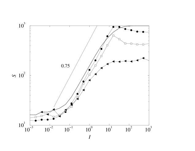
FIG. 3.: Average number of species at equilibrium in the IBM model as a function of the immigration rate $I$. Three different regimes are observed as $I$ is increased. The parameters for each of the curves are: $N_{h}=10^{4}$, $M_{h}=100$, $M_{a}=900$, $E=100$, $E_{rep}=200$, $\ell=3$, $b=5$, $d=2$, $\delta=20$, $p_{d}=0.002$ (solid triangles); empty squares correspond to the same parameters with $d=1$, and solid circles to the same situation but $E=150$, $b=10$, and $d=1$. This three curves have been obtained from random matrices (RM). The solid line corresponds to a simulation of the CM with parameters as in the last case.

The results for the continuous model are completely similar. The regime between the two plateaus is represented in Fig. 4. Notice that in this case we do not have a fixed continental pool, or, in other words, the parameter $M$ has to be interpreted as infinite. Some of the curves show a curvature in log-log plots, which can be eliminated introducing $S_{0}$ as additional fit parameter and plotting ($S-S_{0}$) versus $I$. The effect of $S_{0}$ is thus to reduce the effective exponent $a$ as the immigration flux is reduced.

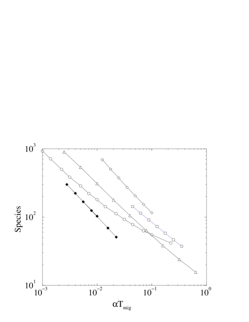
FIG. 4.: Sample of plots of the stationary number of species as a function of the inverse of the immigration rate, $T_{\rm mig}$, in units of $1/\alpha$. Filled symbols refer to simulations of model (A) Eq. (3), empty symbols are for model (B). Parameters are as follows. Filled diamonds: $N^{\prime}_{c}=10^{3}$, $\beta^{\prime}=10^{3}$, $\gamma^{\prime}_{\rm max}=5\cdot 10^{3}$ (in this case the horizontal axis is $10\alpha T_{\rm mig}$). Empty circles: $N^{\prime}_{c}=10^{5}$, $\beta^{\prime}=10^{2}$, $c^{\prime}_{\rm max}=20$. Empty diamonds: $N^{\prime}_{c}=10^{4}$, $\alpha=0$, $c_{\rm max}/\beta R=20$ (in this case the horizontal axis is $T_{\rm mig}/\beta R$). Empty squares: $N^{\prime}_{c}=3.2\cdot 10^{6}$, $\beta^{\prime}=32$, $c^{\prime}_{\rm max}=2$. Empty triangles: $N^{\prime}_{c}=10^{5}$, $\beta^{\prime}=2$, $c^{\prime}_{\rm max}=8$. $\ell_{\rm max}$ is either four or eight. In all cases, $N_{\rm ini}=4N_{c}$.

The observed exponents range from $a=0.42$ to $a=1$. Interestingly, the case with $a=1$, corresponding to a competition exponent $b=0$ (not represented in Fig. 4), refers to a case where basal species were not in competition, since we used constant parameters $\gamma_{ij}$ and constant resources $N_{0}(t)\equiv R$. In all other cases the exponent $b$ was positive.

We now discuss shortly the behavior of biodiversity with the parameters of the ecological equations. Keeping fixed the other dimensionless parameters given in Eqs. (8) and (9), biodiversity increases logarithmically with the resources $R/N_{c}$:

$$S\approx A_{1}+A_{2}\log\left(R/N_{c}\right)\,.$$ (13)

This result holds for the IBM and for the continuous models, but for model (A) it is only valid in some range of parameter values. In fact, model (A) at fixed $\gamma^{\prime}_{max}$ is found, for large $R/N_{c}$, in the garden regime, where only basal species survive, and the scaling behavior is different there (see Appendix). The exponent $a$, defined in Eq. (10), changes only very weakly with $R/N_{c}$.

Biodiversity also increases with the maximal transfer rate, either $c^{\prime}_{\rm max}$ for the case of Eq. (6) or $\gamma^{\prime}_{\rm max}$ for model (A), when all other parameters in Eq. (8) are kept constant. In the first case, the number of species tends to zero as $c^{\prime}_{\rm max}$ approaches unity (for $N_{\rm ini}=N_{c}$). In the second case, at small $\gamma^{\prime}_{\rm max}/N^{\prime}_{c}$ we reach the “garden regime” (see Appendix) where the number of species is almost independent of $T_{\rm mig}$. Both limits can be interpreted as corresponding to $a=0$, thus $b=\infty$. The exponent $a$ then increases slowly with $\gamma_{\rm max}$.

The effect of the parameter $\beta^{\prime}$, when other parameters in Eqs. (8) and (9) are fixed, depends on the immigration rate. While biodiversity increases for increasing $\beta^{\prime}$ at small immigration, the opposite happens if immigration is large. Thus, $I-S$ curves relative to different values of $\beta^{\prime}$ should cross at some point. This behavior reflects on the fact that the exponent $a$ decreases with increasing $\beta^{\prime}$, while $S_{0}$ increases. As in the case of $\gamma^{\prime}_{\rm max}$, the decrease of $a$ can be explained by the fact that, at larger $\beta^{\prime}$, the probability that a colonizer has a positive growth rate becomes smaller. The positive effect on $S_{0}$, on the other hand, is due to the fact that the larger $\beta^{\prime}$, the more likely that two predators feeding on the same prey species can coexist.

We also measured the whole stationary distribution of the number of species $s$, $P(s)$. We plot in Fig. 5a the ratio between the variance $V_{s}=\langle s^{2}\rangle-\langle s\rangle^{2}$ and the mean $S=\langle s\rangle$ as a function of the mean number of species $S$. The measure is much noisier than that of the average value, and it is strongly affected from possible sampling errors. The variance is typically lower than the mean for small $\langle s\rangle$, but at some point increases faster than the mean, becoming larger than it at large $\langle s\rangle$. Since for a Poissonian distribution the variance and the mean are equal, the distribution $P(s)$ is narrower than a Poissonian one for small $\langle s\rangle$ and broader than it for large $\langle s\rangle$ (see Fig. 5b, where for each curve a Poissonian distribution with the same mean value has been represented as a dashed line). Notice however that the comparison with a Poissonian distribution is very good for some range of parameters.

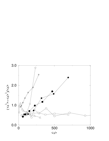
FIG. 5.: (a) Ratio between the variance and the mean of the distribution of the number of species. (b) Comparison of four stationary $P(s)$ (solid lines) with Poissonian distributions with the same average value (dashed lines). From left to right resources and immigration rate increase with the other parameters fixed. Model (B) of the continuous dynamics has been used.

B Species area relationship

In order to investigate the dependence between biodiversity and area, we have to fix the relationship between area and immigration rate $I$. Usually, a positive correlation is expected even though the actual dependence may vary with the species considered. We restrict our study to the assumption that the immigration rate is proportional to the linear size of the island (MacArthur & Wilson, 1963):

$$I=1/T_{\rm mig}=I_{0}+kA^{1/2}\>.$$ (14)

We also include a constant $I_{0}$ to take into account that, for islands in an archipelago, the immigration rate depends much more on the geometry of the archipelago and on its distance from the mainland than on the value of the area. For isolated islands and whole archipelagos, on the other hand, there is usually a unique source of immigrants from the mainland, and the effect of area on immigration is expected to be important. In view of this situation, in the first part of the discussion the constant $I_{0}$ will be neglected. The parameter $k$ is related to the distance from the mainland.

In the framework of the IBM, the other parameter influenced by area is the number of patches $N_{h}$, which is taken to be proportional to area: $N_{h}=A$, with an appropriate choice of units. Thus we simulated systems with different values of $N_{h}$, varying the immigration rate as above. Our main result is that we always obtain a power-law dependence of the number of species with the area, with typical values of $z$ in the interval $0.6-0.8$, as it is observed for the case of archipelagos, to which our immigration model should apply. Taking into account additional sources of immigrations, like closeby islands, is expected to reduce the dependence of the immigration rate on area, and thus to cause a decrease of the effective $z$ values, making them more similar to the values observed in groups of neighboring islands.

For the IBM, we represent in Fig. 6 the number of species as a function of area, with immigration rate $I\equiv k\sqrt{A}$ and $N_{h}\equiv A$, for different values of the continental pool $M$. It can be seen that the species area relationship bends for large areas, apparently tending to an asymptote. Increasing the species pool $M$ increases the asymptote, but leaves the value of the effective exponent unchanged. Parameter values are $E=150$, $E_{rep}=200$, $d=1$, $\delta=20$, $p_{d}=0.002$ and $k=0.353$.

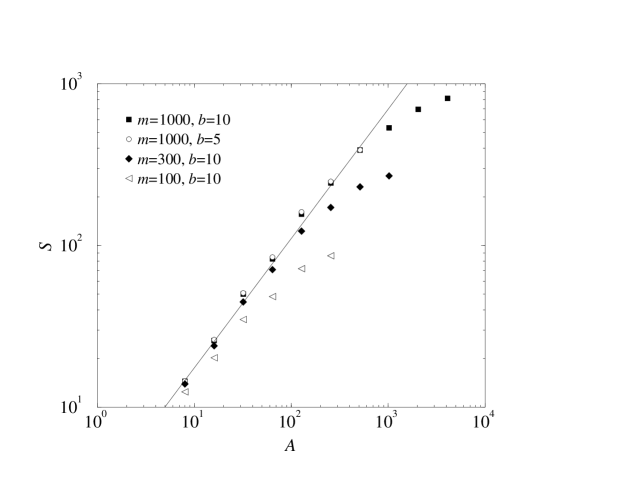
FIG. 6.: Average number of species as a function of area in the IBM model, for an immigration rate proportional to the square root of $A$. The three curves correspond to different sizes of the species pool $M$, as shown in the legend. The remaining parameters are equal for the three curves and are $E=150$, $E_{rep}=200$, $d=1$, $\delta=20$, $p_{d}=0.002$. The straight line is given by $z\sim 0.75$. This results are obtained with the cascade model. Similar curves are obtained for a random matrix, with values of $S$ slightly below these, on the average.

We now come to the species-area relationship in the continuous formulation of the ecological dynamics. We should first discuss how the parameters of the ecological equations, Eqs. (8) and (9), depend on area. The variables $N_{i}$ of ecological equations have the meaning of spatial densities of individuals. Thus the equations Eq. (3) are invariant with respect to changes of area. There is however another important determinant of the ecological dynamics: The threshold $N_{c}$ below which extinctions happen. Two different cases have to be considered:

1. $N_{c}$ independent of area, in other words there is a critical density below which the species go extinct, as it happens for the Allee’s effect (Allee et al., 1949). Such a situation is expected, for instance, if the individual of the species are uniformly dispersed in the area $A$ so that, below the critical density $N_{c}$, they can not find mating partners.

   In this case, the ecological dynamics is invariant under changes of the area and, in particular, the extinction rate does not depend on $A$. Assuming that the immigration rate increases with area as in Eq. (14), and that the area is much larger than $(I_{0}/k)^{2}$, we find

   $$S\propto A^{z}\>,\>\>\>\>\>z=a/2\>,$$ (15)

   where $a$ is the exponent in Eq. (10).

2. Extinctions depend on the absolute number of individuals, $N_{i}A$ and the extinction threshold is thus

   $$N_{c}\propto 1/A\,.$$ (16)

   1. First we consider this case together with $I=I_{0}$ independent of area (corresponding to $k=0$ in Eq. (14)). From equation (13), we obtain then that the number of species increases logarithmically with area:

      $$S\approx A_{1}+A_{2}\log(A)\,.$$ (17)

      This relation is indeed observed for birds in the central islands of the Solomon archipelago, which are all very close to at least one other large central islands (Diamond & Mayr, 1976). For such islands, the immigration rate can be expected to be rather independent of area.

   2. Extinctions depend on the absolute number of individuals and the immigration rate increases with island size $(A\gg(I_{0}/k)^{2})$,

      $$N_{c}\propto 1/A\,,\>\>\>\>\>\>I=kA^{1/2}\,.$$ (18)

      In this case, we can not rely on previous results, and we have to perform new simulations, scaling the parameters as in Eq. (18).

We note that, in both cases 2(a) and 2(b), model (A) can become problematic at large area. In fact, as area increases the coupling constant $\gamma_{\rm max}N_{c}/\alpha\propto 1/A$ becomes smaller, and the system becomes dominated by dissipative effects. The result is that, unless $\alpha=0$, Eq. (29) in the Appendix would not be satisfied as area increases, and the system would meet a “garden regime”, in which only basal species survive (see Appendix). It is not surprising that Lotka-Volterra equations go in trouble for very low densities: in fact, they are analogous to equations of chemical kynetics, and when the density of the species involved becomes too small, the assumptions on which they are founded break down. To avoid such a problem, we used the ratio dependent model (B) together with Eq. (18). Nevertheless, our numerical study shows that also model (A) provides comparable results in a suitable range of parameters.

Results are plotted in Fig. 7, and yield an approximately power law species area relationship, for large enough values of the parameter $\alpha k$. In the log-log plot, the curves $S(A)$ show a negative curvature, that can be eliminated introducing a new parameter $A_{0}$,

$$S\approx c(k)\left(A-A_{0}(k)\right)^{z(k)}\>.$$ (19)

Both the effective exponent $z(k)$ and the limit area $A_{0}(k)$ increase slowly with the immigration parameter $k$. For the curves in Fig. 7, the exponent $z(k)$ ranges from $z=0.49$ at $k=2$ to $z=0.56$ at $k=50$.

We notice however that the scaling form Eq. (19) is only approximate, that a scaling of the form $A^{z}\log(A)$ would probably be more adequate, and that the immigration rate is a better scaling variable than area. We extract an exponent from our approximately power law species area relationship only for the sake of comparison with field data.

Our model of immigrations applies to whole archipelagos or to isolated islands, because we consider a unique source of immigrations. It is remarkable that the exponent $z$ observed for a set of Pacific archipelagos has the value $z=0.54$ (Adler, 1992; Rosenzweig, 1995), in very good agreement with the results of our simulations. Real data are shown for comparison in Fig. 7b.

It is striking that models at different description levels, as the IBM and the continuous model (B), yield very similar species area relationships. We compared other statistical features of the individual based and the continuous models, finding that they are qualitatively very similar (this holds for the Lotka-Volterra model as long as the garden regime and the opposite low dissipation regime are avoided). In the following we will present a complete analysis of the stationary state for data obtained from the IBM and from model (B).

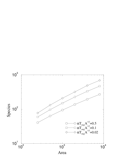
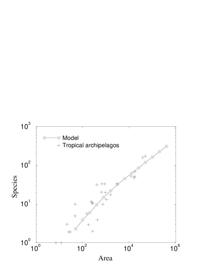
FIG. 7.: Number of species as a function of area, in the hypothesis $R\propto A$, $T_{\rm mig}=kA^{-1/2}$. (a) Curves for different values of $k$. (b) A curve for $k=0.02$ compared to biodiversity data of Pacific archipelagos (Adler, 1992; Rosenzweig, 1995). The frequency dependent continuous equations, Eq. (6), have been used. Empty symbols refer to $\ell_{\rm max}=4$, filled symbols to $\ell_{\rm max}=8$.

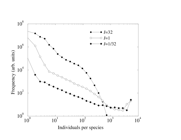
FIG. 8.: Distribution of the number of individuals per species in the IBM model for different values of the immigration rate. The remaining values are as in Fig. 3. As can be seen, the abundances of species are power-law distributed with an exponent close to unity in all cases. The increase in the immigration rate moves the exponential cut-off at large sizes towards the left.

C Distribution of species abundances

We measured distributions of species abundances, defined as the probability density $p(N)$ of species with $N$ individuals (or total biomass equal to $N$ in the case of the continuous model), both for the IBM and for the continuous model. We observe a good qualitative agreement of the results in both approaches.

In the framework of the IBM, we measured the distribution of species abundances for three values of the immigration rate corresponding to the three regimes in Fig. 3 (slow, intermediate and fast driving). Fig. 8 represents the frequency $p(N)$ with which species formed by $N$ individuals were recorded. Different curves refer to different immigration rates (other parameters as in Fig. 3). All curves show an initial fast decaying part corresponding to species that go extinct almost immediately after arriving to the island. Since these species do not find preys to feed on, their initial energy decays exponentially and they die out of starvation. The relevant part of these distributions results from species which play a role in the ecological network. This part shows a power-law decay of the form

$$p(N)\propto N^{-\xi}\;,$$ (20)

with $\xi\simeq 1$. Finally, the external resources set the value of $N$ at which an exponential cut-off appears. Our results are in good agreement with field measures of diversity, many of which also return a power-law distribution of species abundances with an exponent in the range $1-1.25$ (Pielou, 1969; Solé et al., 2000).

The same results are obtained in the framework of the continuous model. In this case, however, we observe that the exponent $\xi$ increases slowly with immigration rate, tending to $\xi\approx 1$ in the limit $I\rightarrow 0$. The maximum value that we found in our simulations is $\xi\approx 1.25$, still compatible with observational data. A sample of results is reported in Fig. 9a. In Fig. 9b the decrease of the exponent $\xi$ with the immigration rate is shown.

FIG. 9.: (a) Distribution of the biomass per species in the continuous model (B), for different values of the immigration rate. Other parameters: $N^{\prime}_{c}=10^{5}$, $\beta^{\prime}=1$, $c^{\prime}_{\rm max}=2$, $\ell_{\rm max}=4$. (b) The exponent $\xi$ of the power-law part of the distribution minus one as a function of the immigration rate. Same parameters as in the previous part.

D Lifetime distribution

The distribution of lifetimes of species is shown in Fig. 10 in a log-log plot, for several values of the immigration rate and of other parameters. After an initial part where the distribution is almost uniform, corresponding to species with very short permanence time, we observe an approximately power law decay of the probability density for a range of at least one and half decade

$$p(\tau)\approx\tau^{-\eta}\>,$$ (21)

when using different parameter values, we found values of the effective exponent $\eta$ between 2.1 and 2.8.

The average lifetime $\langle\tau\rangle$ in the equilibrium state is related to biodiversity through the relation

$$\langle\tau\rangle=T_{\rm mig}\langle S\rangle\propto T_{\rm mig}^{b/(1+b)},$$ (22)

which follows from its definition and from the properties of the stationary state. Here $T_{\rm mig}$ represents the average time between succesful immigrations which contribute to the island biodiversity. Thus the average lifetime decreases with the immigration rate $1/T_{\rm mig}$ and, consistently, the value of the exponent increases, as it is shown in Fig. 10b.

Our results compare qualitatively well with observed patterns (Keitt & Marquet, 1996; Keitt & Stanley, 1998). It was in fact observed that the time of permanence of birds in local patches follow a distribution approximately of the form (21) with effective exponent $\eta=1.6$, indeed smaller than the typical values found in our simulations. A result which compares better to this last value has been found, using a model without explicit ecological dynamics, in (Solé et al., 2000).

FIG. 10.: (a) Distribution of the lifetimes in the continuous model (B), for different values of the immigration rate. Other parameters: $N^{\prime}_{c}=10^{5}$, $\beta^{\prime}=1$, $c^{\prime}_{\rm max}=2$, $\ell_{\rm max}=4$. (b) The exponent $\eta$ of the power-law part of the distribution as a function of the immigration rate. Same parameters as in the previous part.

E Network organization

The structure of the ecological network does change, even if very slowly, with changing immigration rate. We have examined in particular the number of trophic levels, the number of links per species and the total biomass.

We define the trophic level of a species as the minimal number of links connecting it to resources. In all our simulations the number of trophic levels varies between four and ten. It shows a tendency to increase with immigration rate, as it is illustrated in Fig. 11.

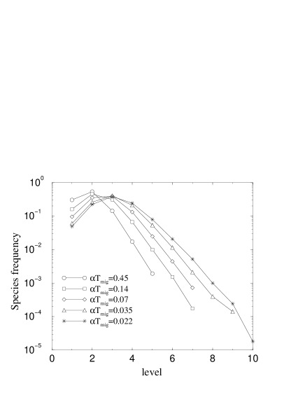
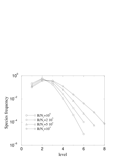
FIG. 11.: (a) Frequency of species at trophic level $l$ in all the course of the simulation in the continuous model (B), for different values of the immigration rate. Food webs become longer at increasing immigration rate. (b) Same, for different values of the resources.

The average number of links per species, counted as average number of preys, is shown in Fig. 12 as a function of the immigration rate. It changes very slowly (logarithmically) and, in some cases, in a non monotonic way (for most curves we only observe either the increasing or the decreasing part). A similar pattern is observed as a function of the resources $R$ (see Fig. 12b). Thus, as a function of the number of species, the number of links per species behave non monotonically. It also depends weakly on the maximum number of links allowed when the new species is added to the ecosystem, $\ell_{\rm max}$.

The total biomass also increases approximately as a power law of the immigration rate, as shown in Fig. 13. The exponent ranges from 0.15 to 0.58.

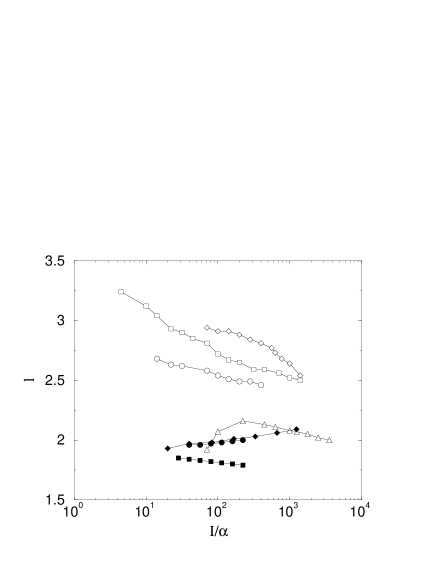
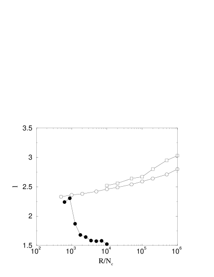
FIG. 12.: (a) Number of links per species as a function of the immigration rate for the continuous model (B). Empty points refer to $\ell_{\rm max}=8$, filled points to $\ell_{\rm max}=4$. (b) Same, as a function of the resources $R$.

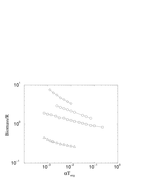
FIG. 13.: Biomass as a function of the inverse of the immigration rate, $T_{\rm mig}$, in the continuous model (B).

V Relationship to MacArthur & Wilson’s theory

We have already seen in the previous section that quantitative biodiversity patterns can be derived from a balance between external driving through immigrations and the intrinsic population dynamics of the ecosystem. Here we want to relate these results to existing phenomenological approaches, in particular MacArthur and Wilson’s (1963, 1967) theory of island biogeography.

In an ensemble average (or, equivalently, in an average over long times), the response of the system to a constant immigration flux $I$ reduces to a stationary extinction $E$. This can be expressed as a function of the avergage number of species $S$ in the system, $E=E(S)$. Of course, this function depends also on the model paramenters and on qualitative features of the immigration flux. Since the system is in a stationary state, immigration and extinction have to compensate each other on average:

$$I-E(S)=0\;.$$ (23)

This balance is indeed as postulated by MacArthur and Wilson. The immigration flux measures the average number of new species arriving per unit of time. The functional form of the ‘extinction curve’ $E(S)$ can now be obtained from the underlying population dynamics. As explained above, we find

$$E(S)\,=\,E_{0}S^{1+b}\,,$$ (24)

in the scaling regime where the number of species increases as a power-law of the immigration rate. The exponent $b$ was called competition exponent and has been introduced in Eqs. (11) and (12). In fact, from the stationary solution of Eq. (23), we recover Eq. (10)

$$S\,=\,\left(\frac{I}{E_{0}}\right)^{\frac{1}{1+b}}\,.$$ (25)

This equation allows to derive the exponent $z$ of the species-area relationship. Indeed, if we assume that

$$I\propto A^{s}\;,\>\>\>\>\>\>\>E_{0}\propto A^{-\epsilon}\>,$$ (26)

we find

$$S\propto A^{z}\;,\>\>\>\makebox{with}\>\>\>\>z={s+\epsilon\over 1+b}\>.$$ (27)

For the population models, we assumed $s=1/2$ (the immigration rate is considered proportional to the linear size of the island), and we obtained $\epsilon=0$ (in fact, the number of species increases as the logarithm of $R/N_{c}$ at fixed $T_{\rm mig}$, both in the IBM and in the continuous model (B)).

We remark that here, as in the explicit population models, we are assuming that the only source of immigrants is a continent far apart. The exponents that we find should then be compared to the exponents observed for isolated islands or archipelagos, while the exponent computed among islands of the same archipelago is expected to be lower, due to a reduced dependence of immigration rate on area. Another point to remark is that the immigration rate $I$ measures the flux of new species arriving on the island. If this flux is assumed to originate from a ‘continent’ of $M$ species, $I$ can be related to the total immigration flux $I_{0}$ by correcting for the immigrations already present on the island. The simplest ansatz is $I(S)=I_{0}(1-S/M)$ (MacArthur and Wilson, 1963, 1967). Expressed in terms of $I_{0}$, the average number of species $S$ reaches a saturation value of order $M$. (The pool of immigrant species is indeed finite in our IBM, but infinite in the continuum models. Hence, this correction becomes important in comparing results of the different models).

VI Summary and Conclusions

We have presented a study of biodiversity in an insular ecosystem at the individual and the population level. Our interest has been focused on the statistical properties of the dynamical stationary state and on the scaling relations between the system variables. Instead of describing detailed situations in which some particular species and their exact interactions with their known preys and predators are included, we let ecological networks self-organize through random assemblage of species, ecological dynamics and possible extinctions.

Our main result is that, in a broad range of parameters, biodiversity scales approximately as a power law of the immigration rate. The value of the exponent varies slightly when the parameters of the models are changed, but the qualitative features of the stationary state are quite robust.

The behavior of biodiversity with immigration rate allows to derive a species area relationship with a power law shape, if we assume that the immigration rate is proportional to the linear size of the island. Such a model of immigration considers as unique source of diversity a flux of species from a continent far apart, thus it should be compared to observations relative to isolated islands or to whole archipelagos. The agreement is in this case rather good: the observed value of the effective exponent $z$ on archipelagos is $z=0.54$ (Adler, 1992; Rosenzweig, 1995), while we typically get, with the continuous model, values between $0.52$ and $0.56$ and, with the individual based model, values between $0.6$ and $0.8$. Thus, the comparison of our two description levels points out to species-area law of the type (1) as a generic feature of a broad set of ecological models with random interactions.

Our models reproduce qualitatively other features observed in real ecosystems. We observe a power law distribution of population abundances, i.e. the number $p(N)$ of species with $N$ individuals approximately decreases as $p(N)\propto N^{-\xi}$. This is expected to be a general consequence of the multiplicative nature of population dynamics equations. The exponent $\xi$ found in our simulations is close to unity, in favourable comparison with field data, and increases with the immigration rate.

We also observe a broad distribution of the time of permanence of species in the system $\tau$, as it has been observed in the field (Keitt & Marquet, 1996; Keitt & Stanley, 1998) and in a related model (Solé et al., 2000). The average permanence time is proportional to the number of species and inversely proportional to the immigration rate, $\langle\tau\rangle=\langle S\rangle T_{\rm mig}$, so that it decreases with the immigration rate. The fact that it is observed, both in field studies and in models, that its distribution is broad, could help to reconcile the apparent dichotomy between fugitive species and permanent species: These groups of species could correspond to the two extreme cases of a unique distribution of permanence times (Schoener & Spiller, 1987). The approximate power law shape of the distribution of times of permanence in the island is reminiscent of the analogous distribution of the lifetime of genera in the fossil record, which is approximately given by $P(\tau)\propto\tau^{-\eta}$, with $\eta\approx 2$, close to what is observed in our model for very small immigration rates and also close to ecological observations. It is tempting to speculate that this similarity points out at similar mechanisms acting on the time scales of ecosystem dynamics as on the timescales of macroevolution.

The number of trophic levels in the food web is also strongly influenced by the immigration rate. We typically find from four to ten trophic levels, depending on parameters, and with a tendency for the number of levels to increase with immigration rate. Hints to the correlation between immigration rate and number of levels can be found in the fact that the length of food chains appears to be positively correlated to habitat area, although the data are quite poor (Schoener, 1989; Spencer, 1997). Our results suggest that one of the factors limiting the length of food chains is the immigration or speciation rate. Notice that in our model no other limitations to the length of food chains exist: energetic considerations would limit the number of levels to a value $\log(R/N_{c})$, much larger than the one observed.

An important result of our study is that the observed statistical patterns are rather robust with respect to changes in the dynamical rules of the model. One example is the representation of space in the IBM model. Although one could think that in this case explicit space is needed, we modelled space only in an effective way, increasing the immigration rate and the resources with the area. We believe that this effective approach captures the main features of the behavior of biodiversity with area, even if important issues, like for instance the presence of many different habitats, are not represented in the model.

As Pimm poses it, (…) it is pointless to try to justify models’ equations biologically – their assumptions are almost bound to be wrong. (…) The concern should not be whether the assumptions are wrong (they are!), but whether it matters that they are wrong. (Pimm, 1991). It seems that the statistical laws and the scaling relationships that we observed are generic properties of complex ecosystems, that is an unavoidable results of a minimal set of rules governing population dynamics and immigrations. Thus the strategy is to look for the simplest set of rules which appear sensible and which allow to derive the observed statistical patterns of biodiversity.

Appendix. The garden regime

In the case of model (A) of continuous dynamics, we observed that only basal species could survive on the long run for parameter values in a certain range. In this case, observing the system on a very long time scale, we did not see any stationary state (although a stationary state was reached for a much smaller system), but we saw a number of species steadily and slowly increasing in time (see Fig. 14).

We call such a regime the garden regime, since predators are absent. Its statistical properties are peculiar: the distribution of biomasses is narrow and peaked at very low values, and the distribution of lifetimes is bimodal, with a high peak for very short lifetimes corresponding to non-basal species, and a shorter one for large lifetimes, corresponding to basal species. (Even if at any moment there are many more basal species than predators, the number of predators passing through the system and almost immediately going extinct is much larger than the corresponding number of basal species.) Finally, the distribution of the transfer rate $\gamma_{0i}$ from the external resources to species $i$ is strongly peaked close to the maximum allowed value $\gamma_{\rm max}$. All these features can be easily rationalized as follows.

FIG. 14.: Evolution of the number of species in the garden regime. Notice that, although the rate of increase gets slower, the number of species does not reach any stationary value yet. Continuous equations with constant $\gamma_{ij}$’s have been used. Parameters: $\gamma N_{c}/\alpha=0.1$, $\beta^{\prime}=10$, $N^{\prime}_{c}=1000$, $\ell_{\rm max}=4$.

Let us consider a situation where $S$ basal species coexist feeding on the abiotic resources $N_{0}$. Our calculations (unpublished) show that at the static fixed point of the corresponding ecological equations, Eqs. (3) and (4), all biomasses are positive if and only if all differences in the coefficients $\gamma_{0i}$ are smaller than $B/S$, where $B=\gamma_{0}\beta R/\alpha$. Thus, as $S$ increases, the coupling constants between the basal species and the environment deviate from the initial distribution and become more and more similar. Notice that, if $\beta=0$, the coefficients $\gamma_{0i}$’s should be exactly equal to guarantee coexistence (this expresses in this context the “principle of competitive exclusion”). This conclusion does not vary qualitatively if one considers Eq. (6) instead of the model with constant coefficients $\gamma_{ij}$. Thus, in a system without predators and high immigration of basal species, we would expect to find many basal species with very similar biomasses, all of order $R/S$ ($S$ should be smaller than $R/N_{c}$) and coefficients $\gamma_{0i}$ very close one to each other in value.

Let us now consider the arrival of a predator to such a system, considering first Lotka-Volterra equations (model (A)). The rate of growth of the predator cannot be larger than $r_{\rm max}$ given by

$$r_{\rm max}=\ell_{\rm max}\gamma_{\rm max}{R\over S}-\alpha-\beta N_{c}.$$ (28)

Since $R/S$ is larger than $N_{c}$, we find that, for large $S$, a non-basal species can colonize only if

$$\gamma_{\rm max}\geq{1\over\ell_{\rm max}}\left({\alpha\over N_{c}}+\beta\right)\,.$$ (29)

Every time we observed in our simulations ecosystems mainly composed of basal species and whose biodiversity has a time behavior similar to that in Fig. 14, the above condition was not fulfilled.

In model (B), Eq. (6), $r_{\rm max}$ equals $\ell_{\rm max}\alpha^{\prime}c_{\rm max}-\alpha-\beta N_{c}$. This quantity must be larger than zero, otherwise no species would survive. Thus the “garden regime” that we described in this appendix can not be found in simulations of ratio dependent functional responses, unless we decide to use different parameters for basal and non-basal species.

Parameter	Meaning	Value-Range
$p_{d}$	Death probability	0.001-0.02
$d$	Dissipation rate	1-10
$N_{h}$	Max. Ind. in basal species ($\simeq$ island area)	100-10000
$b$	Basal growth	2-25
$C(m_{i},m_{j})$	Energy obtained by $i$ when eating $j$	max. $E\in[20,200]$
$E_{rep}$	Reproduction energy	100-300 ($E_{rep}\approx 2E$)
$\delta$	Energy when born	5-$E/2$
$\ell$	Number of preys per predator	3-4
$M_{h}$	Max. number of basal species	1-100 or CM
$M_{a}$	Max. number of animal species	1-1000
$I$	Immigration rate	$10^{-3}-10^{3}$

TABLE I.: Parameters in the IB model and values used.

REFERENCES

- [1] Abrams, P.A. & Ginzburg, L.R. (2000). The nature of predation: prey dependent, ratio dependent or neither? Trends in Ecol. Evol. 15, 337-341.
- [2] Adler G.H. (1992). Endemism in birds of tropical Pacific islands, Evol. Ecology 6, 296-306.
- [3] Allee, W.C., Emerson, A.E., Park, O., Park, T. & Schmidt, K. (1949). Principles of animal ecology, Saunders, Philadelphia.
- [4] Arditi, R. & Ginzburg, L.R. (1989). Coupling in predator-prey dynamics: ratio dependence. J. theor. Biol. 139, 311-326.
- [5] Arditi, R. & Michalski, J. (1995). Nonlinear food web models and their responses to increased basal productivity, in: Polis, G.A., Winemiller, K.O. (Eds), Food Webs: Integration of Patterns and Dynamics. Chapman and Hall, London.
- [6] Banavar, J.R., Green, J.L., Harte, J., & Maritan, A. (1999). Finite size scaling in biology. Phys. Rev. Lett. 83, 4212-4214.
- [7] Bascompte, J., Solé, R.V., & Martínez, N. (1997). Population cycles and spatial patterns in snowshoe hares: An individual-oriented simulation. J. Theor. Biol. 187, 213-223.
- [8] Begon, M., Harper, J.L., and Townsend, C.R. (1998). Ecology. Blackwell Science Ltd, Oxford.
- [9] Berger, U., Wagner, G., & Wolff, W.F. (1999). Virtual biologist observe virtual grasshoppers: an assessment of different mobility parameters for the analysis of movement patterns. Ecol. Mod. 115, 119-127.
- [10] Biham, O., Malcai, O., Levy, M. & Solomon, S. (1998). Generic emergence of power law distributions and Lévy stable intermittent fluctuations in discrete logistic systems. Phys. Rev. E 58, 1352-1358.
- [11] Caldarelli, G., Higgs, P.G., & McKane, A.J. (1998). Modelling coevolution in multispecies communities. J. theor. Biol. 193, 345-358.
- [12] Case, T.J. (1990), Invasion resistance arises in strongly interacting species-rich model competition communities. Proc. Natl. Acad. Sci. USA 87, 9610-9614.
- [13] Cohen, J.E., Briand, F., & Newman, C.M. (1990). Community food webs. Biomathematics Volume 20, Springer-Verlag, Berlin Heidelberg.
- [14] Cohen, J.E. & Newman, C.M. (1985). When will a large complex system be stable? J. theor. Biol. 113, 153-156.
- [15] Diamond, J.M. & Mayr, E. (1976). Species-area relation for birds of the Solomon archipelago. Proc. Natl. Acad. Sci. USA 73, 262-266.
- [16] Drake, J.A. (1990). The mechanics of community assembly and succession. J. theor. Biol. 147, 213-233.
- [17] Drossel B., Higgs P.G. & McKane, A.J. (2000). The influence of predator-prey population dynamics on the long-term evolution of food web structure. Preprint arXiv:nlin.AO/0002032.
- [18] Durrett, R. & Levin, S. (1996). Spatial models for species-area curves. J. theor. Biol. 179, 119-127.
- [19] Fahse, L., Wissel, C., and Grimm V. (1998). Reconciling classical and individual-based approaches in theoretical population ecology: A protocol for extracting population parameters from individual-based models. Am. Nat. 152 838-852.
- [20] Gilpin, M.E. & Diamond, J.M. (1976). Calculation of immigration and extinction curves from the species-area-distance relation. Proc. Natl. Acad. Sci. USA 73, 4130-4134.
- [21] Gilpin, M.E. & Diamond, J.M. (1980). Turnover Noise: Contribution to Variance in Species Number and Prediction from Immigration and Extinction Curves. Am. Nat. 115, 884-889.
- [22] Gilpin, M.E. & Diamond, J.M. (1981). Immigration and Extinction Probabilities for Individual Species: Relation to Incidence Functions and Species Colonization Curves. Proc. Natl. Acad. Sci. USA 78, 392-396.
- [23] Grimm, V., Wyszomirski, T., Aikman, D., & and Uchmański, J. (1999). Individual-based modelling and ecological theory: Synthesis of a workshop. Ecol. Mod. 115, 275-282.
- [24] Hall S. & Halle, B. (1999). Modelling activity synchronization in free-ranging microtine rodents. Ecol. Mod. 115, 165-176.
- [25] Happel R. & Stadler, P.F. (1998), The evolution of diversity in replicator networks. J. theor. Biol. 195, 329-338.
- [26] Harte, J., Kinzig, A., & Green, J. (1999). Self-similarity in the distribution and abundance of species. Science 284, 334-336.
- [27] He, F. & Legendre, P. (1996). On species-area relations. Am. Nat. 148, 719-737
- [28] Heatwole, H. & Levins, R. (1972). Trophic structure stability and faunal change during recolonization. Ecology 53, 531-534.
- [29] Holling, C.S. (1959). Some characteristics of simple types of predation and parasitism. Can. Ent. 91, 385-398.
- [30] Humboldt, F.H.A. (1807). Essai sur la geographie des plantes. Sherborn Fund facsimile, no. 1, Society for the Bibliography of Natural History, London 1959.
- [31] Keitt, T.H. (1997). Stability and complexity on a lattice: Coexistence of species in an individual-based food web model. Ecol. Mod. 102, 243-258.
- [32] Keitt, S.H. & Marquet, P.A. (1996). The Introduced Hawaiian Avifauna Reconsidered: Evidence for Self-Organized Criticality? J. theor. Biol. 182, 161-167.
- [33] Keitt, S.H. & Stanley, H.E. (1998). Dynamics of North American breeding bird populations. Nature 393, 257-260.
- [34] Kerner, E.H. (1957). A statistical mechanics of interacting biological species. Bull. Math. Biophys. 19, 121-146.
- [35] Łomnicki, A. (1999). Individual-based models and the individual-based approach to population ecology. Ecol. Mod. 115, 191-198.
- [36] Loreau, M. & Mouquet, N. (1999). Immigration and the maintenance of local species diversity. Am. Nat. 154 427-440.
- [37] MacArthur, R.H. and Wilson, E.O. (1963). An equilibrium theory of insular zoogeography. Evolution 17 373-387.
- [38] MacArthur, R.H. and Wilson, E.O. (1967). The theory of island biogeography. Princeton University Press, Princeton, N.J.
- [39] Manne, L.L., Pimm, S.L., Diamond, J.M., & Reed, T.M. (1998). The form of the curves: a direct evaluation of MacArthur & Wilson’s classic theory. Journal of Animal Ecology 67 784-794.
- [40] May, R. (1972). Will a large complex system be stable? Nature 238, 413-414.
- [41] Morton, R.D. & Law, R. (1997) Regional species pool and the assembly of local ecological communities. J. theor. Biol. 187, 321-331.
- [42] Pelletier J.D. (1999). Species-Area Relation and Self-Similarity in a Biogeographical Model of Speciation and Extinction. Phys. Rev. Lett. 82, 1983-1986
- [43] Pielou, E.C. (1969). An introduction to mathematical ecology. Wiley.
- [44] Pimm, S.L. (1991). The balance of Nature? The University of Chicago Press, Chicago.
- [45] Post, W.M. & Pimm, S.L. (1983). Community assembly and food web stability. Math. Biosci. 64, 169-192.
- [46] Preston, F.W. (1962). The canonical distribution of commonness and rarity. Ecology 43, 185-215, 410-432.
- [47] Rosenzweig, M.L. (1995). Species diversity in space and time. Cambridge University Press, New York.
- [48] Rosenzweig, M.L. (1999). Heeding the warning in biodiversity’s basic law. Science 284, 276-277. See Ref. [1] there (Humboldt, 1807).
- [49] Schoener, T.W. & Spiller, D. (1987). High population persistence in a system with high turnover. Nature 330, 474-477.
- [50] Schoener, T.W. (1989). Food webs from the small to the large. Ecology 70, 1559-1589.
- [51] Schreiber, S.J. & Gutierrez, A.P. (1998). A supply/demand perspective of species invasions and coexistence: applications to biological control. Ecol. Mod. 106, 27-45.
- [52] Simberloff, D.S. & Wilson, E.O. (1969). Experimental zoogeography of islands: The colonization of empty islands. Ecology 50, 278-296.
- [53] Simberloff, D.S. (1969). Experimental zoogeography of islands: a model for insular colonization. Ecology 50, 296-314.
- [54] Solé, R.V., Gamarra, J.G.P., Ginovart, M., & López D. (1999). Controlling chaos in ecology: From deterministic to individual-based models. Bull. Math. Biol. 61, 1187-1207.
- [55] Solé, R.V., Alonso, D., & McKane, A. (2000). Connectivity and Scaling in S-species Model Ecosystems. Physica A, to appear. Also preprint adap-org/9907010.
- [56] Sornette D. (1998). Linear stochastic dynamics with nonlinear fractal properties. Physica A 250, 295-314.
- [57] Spencer, M. (1997). The effects of habitat size and energy on food web structure: An individual-based cellular automata model. Ecol. Mod. 94, 299-316.
- [58] Svirezhev, Yu.M. (1997). On some general properties of trophic networks. Ecol. Mod. 99, 7-17.
- [59] Whittaker, R.J. (1992). Stochasticism and determinism in island ecology. J. Biogeogr. 19, 587-591.
- [60] Williamson, M. (1989). The MacArthur and Wilson theory today: true but trivial. J. Biogeogr. 16, 3-4.
- [61] Wilson, W.G. (1998). Resolving discrepancies between deterministic population models and individual-based simulations. Am. Nat. 151, 116-134.
- [62] Wissel, C. (1992). Aims and Limits of Ecological Modelling Exemplified by Island Theory. Ecol. Mod. 63, 1-12.