Population dynamics advected by chaotic flows:
a discrete-time map approach.

Abstract

A discrete-time model of reacting evolving fields, transported by a bidimensional chaotic fluid flow, is studied. Our approach is based on the use of a Lagrangian scheme where fluid particles are advected by a $2d$ symplectic map possibly yielding Lagrangian chaos. Each fluid particle carries concentrations of active substances which evolve according to its own reaction dynamics. This evolution is also modeled in terms of maps. Motivated by the question, of relevance in marine ecology, of how a localized distribution of nutrients or preys affects the spatial structure of predators transported by a fluid flow, we study a specific model in which the population dynamics is given by a logistic map with space-dependent coefficient, and advection is given by the standard map. Fractal and random patterns in the Eulerian spatial concentration of predators are obtained under different conditions. Exploiting the analogies of this coupled-map (advection plus reaction) system with a random map, some features of these patterns are discussed.

The spatial structure of passive fields transported by a fluid flow is an important question in fluid and nonlinear dynamics. Many important situations require in addition to take into account chemical or biological interactions between the substances transported by the flow. In particular, our motivation comes from the general question on the mechanisms for plankton inhomogeneity in the ocean, and more specially for the spatial patterns that would be reached by plankton or marine hervibores grazing from a localized source of nutrients. We present a general methodology, based in coupled discrete-time dynamical systems describing reaction or population dynamics and advection in the Lagrangian framework, and apply it to a model of logistic population dynamics in the presence of a localized source of nutrients and chaotic advection. Fractal and random spatial features develop in the concentration patterns, which can be understood in terms of an analogy with random maps.

I INTRODUCTION

Patchiness, or the uneven distribution of substances of organisms, is ubiquitously observed in the ocean [1, 2, 3, 4]. In complex situations such as the marine ecosystems, characterized by the interplay of population dynamics and an ambient fluid motion which may differently affect individual populations, the question of how a localized availability of nutrients (or preys, or, in chemical terms, activators) may affect the distribution of primary producers (or predators, or inhibitors, respectively; in the following we refer to preys and predators) is a crucial and challenging problem.

According to [2], the possible causes originating patchiness in marine ecosystems may be grouped in different categories: fluid motion, biological growth coupled with dispersive processes, less ubiquitous mechanisms like swarming, vertical migration, and others. In addition to patchiness, localized availability of food may occur in correspondence of localized sub-ecosystems, such as Posidonia Oceanica beds (for a review see [5]): they display a quite complex structure in which the most important features arise from direct consumption of the plant and epiphyte-herbivore interactions, although a portion of the trophic chain is based on suspended matter [5].

A comprehensive description of such processes leads to the study of the so called advection-reaction-diffusion equations. These are partial differential equations of the type:

$$\frac{\partial C_{i}({\bf x},t)}{\partial t}+({\bf v}({\bf x},t)\cdot\nabla)C_{i}=R_{i}(C_{1},...,C_{N},{\bf x},t)+D_{i}\triangle C_{i}.$$ (1)

Where $C_{i}({\bf x},t)$ ($i=1,...,N$) is the concentration of the $i$-th reactive (in biological or chemical terms) species or substance, and the functions $R_{i}$ describe the reaction, or the population, intrinsic dynamics. The possible explicit spatial and temporal dependence may model the influence of temporal and spatial inhomogeneities in food, temperature, etc. The term $({\bf v}({\bf x},t)\cdot\nabla)C_{i}$ represents advection by a given solenoidal (i.e. incompressible $\nabla\cdot{\bf v}=0$) velocity field ${\bf v}({\bf x},t)$. Finally, the term $D_{i}\triangle C_{i}$ describes diffusion of the $i$-th species or substance with diffusivity $D_{i}$. In writing (1) we are assuming that the evolution of the advected concentrations does not affect that of the underlying flow ${\bf v}({\bf x},t)$. This is definitely reasonable at the scales we are interested in, even though it is worth mentioning that at much smaller scales the presence of organisms may affect the rheological properties of seawater [6, 7].

In some situations it would be necessary to consider a different velocity field for each of the $N$ concentrations $C_{i}$. This may happen, for instance, if different organisms live at different mean depths, leading to differences in the experienced flow. In such cases one has to replace Eq. (1) by

$$\frac{\partial C_{i}({\bf x},t)}{\partial t}+({\bf v}_{i}({\bf x},t)\cdot\nabla)C_{i}=R_{i}(C_{1},...,C_{N},{\bf x},t)+D_{i}\triangle C_{i}.$$ (2)

In this paper, however, we will only consider the case given by Eq. (1) in which the same velocity field advects all the substances.

Introducing the Lagrangian time derivative $\frac{d}{dt}=\frac{\partial}{\partial t}+{\bf v}\cdot\nabla$, Eq. (1) can be written in the form

$$\frac{dC_{i}({\bf x},t)}{dt}=R_{i}(C_{1},...,C_{N},t)+D_{i}\triangle C_{i}.$$ (3)

If diffusion is neglected, it is simple to write the $C_{i}({\bf x},t)$ in terms of the solutions of the Lagrangian evolution equation

$$\frac{d{\bf x}(t)}{dt}={\bf v}({\bf x}(t),t),$$ (4)

and the reactive evolution equation

$$\frac{dC_{i}(t)}{dt}=R_{i}(C_{1},...,C_{N},{\bf x}(t),t).$$ (5)

This set of coupled ordinary differential equations describe the advection-reaction process in a Lagrangian frame: fluid particles move according to (4), and reactions among the $C_{i}$’s occur inside each fluid particle, as expressed by (5), where $C_{i}(t)$ are the concentrations at a particular fluid particle (the one at $x(t)$ at time $t$, i.e. $C_{i}(t)\equiv C_{i}({\bf x}(t),t)$). Denoting by $S^{t}$ and $L^{t}$ the formal solutions of (4) and (5) respectively (i.e., ${\bf x}(t)=S^{t}{\bf x}(0)$ and ${\bf C}(t)=L^{t}{\bf C}(0)$, with ${\bf C}=(C_{1},C_{2},...,C_{N})$) we can write the solution of Eq. (1) in the form (with $D_{i}=0$)

$${\bf C}({\bf x},t)=L^{t}{\bf C}(S^{-t}{\bf x},0).$$ (6)

The case $D_{i}\neq 0$ needs a more elaborated treatment. In addition to the time dependence, $L^{t}$ will have also an explicit space dependence if the $R_{i}$’s have it.

Obviously, the detailed understanding of the above class of partial differential equations constitute a formidable task. However, at this stage of development, we are just interested in the search for generic behaviors expected when few typical characteristics of the flow and of the population dynamics are considered. Thus, if, for example, we concentrate on flows of geophysical nature, horizontal motion turns out to be much more intense than vertical one as soon as one considers scales larger than a few kilometers. This justifies restricting in the following to incompressible twodimensional flows. A turbulent bidimensional flow would be a way to model the irregular advection process to which suspended matter is subjected in real oceans. There are however simpler classes of flows which share some basic characteristics with turbulence, but are much more accessible to analysis: Lagrangian chaotic flows[8, 9]. These are smooth velocity fields, with some simple time dependence in the Eulerian description, but which lead to chaotic trajectories of fluid elements, with the associated stretching and folding, in the Lagrangian description. In this restricted framework, it is well known that even periodic time-dependence in two-dimensional incompressible flows leads generically to chaotic motion of fluid particles.

Rather than integrating the full equations describing the continuous in time dynamics, and since our interest lies mainly in a qualitative characterization of the population system, we will resort in this paper to a discrete in time mapping-approach in terms of discrete-time dynamical systems. This approach is numerically very efficient, and has proven to be extremely productive to study the impact of chaotic advection on mixing [8, 9, 10]. The main idea is to mimic the advection and reaction processes in terms of maps that capture the main features of each aspect. Thus, since we will be looking at processes taking place in 2d incompressible flows, the advective part of our model is naturally described by a twodimensional symplectic map. It is well known that Lagrangian motion in such systems is typically chaotic and with a rather rich behavior. In addition, the transported fluid parcel contains concentrations of active chemical substances or biological specimens subjected to a specific dynamics that will be also modeled in terms of a map. Also, it is worth noticing that even though this is not done in this work, diffusion can be easily reincorporated into the model by averaging, after each iteration of the maps, the concentration of the different species contained in the fluid elements over a region of size $l\sim\sqrt{D_{i}\tau}$, where $D_{i}$ is the corresponding diffusivity and $\tau$ is a characteristic time scale of the system.

The general ideas and formalism sketched above will be made more concrete in the following, and applied to tackle our main problem: the influence of inhomogeneities of the distribution of preys on that of predators. We will make use of some known results for random maps, and compare our discrete-time approach with results obtained in a continuous-time description of the problem [15, 16]. In Section II we will discuss the approach to population dynamics in terms of maps; in Section III our particular model is presented and compared with results for a random logistic map; the analogy helps in the interpretation of the resulting spatial structure of predators, which is described in Section IV, and discussed in Section V.

II A DISCRETE-TIME APPROACH

Let us now present the general idea of our approach for the analysis of the population dynamics in terms of maps.

It is easy to understand that for time-periodic velocity fields, i.e. ${\bf v}({\bf x},t)={\bf v}({\bf x},t+T)$ where $T$ is the period, Eq (4) can be described by a discrete-time dynamical system. The position ${\bf x}(t+T)$ is univocally determined by ${\bf x}(t)$. In addition (because of the periodic velocity field) the map ${\bf x}(t)\to{\bf x}(t+T)$ cannot depend on $t$. Since a periodic time dependence is enough to induce Lagrangian chaos, and because of the above mathematical simplifications, we particularize our study to time-periodic velocity fields, for which we can write

$${\bf x}(t+1)={\bf F}({\bf x}(t)),$$ (7)

Now, time is measured in units of the period $T$. If ${\bf v}$ is incompressible, the map (7) is volume (area in $2d$) preserving, i.e., $\left|\det(\frac{\partial F_{i}}{\partial x_{j}})\right|=1$. In $2d$ the map (7) is symplectic, i.e. the discrete-time version of a Hamiltonian system. Usually, it is not simple at all to obtain ${\bf F}({\bf x}(t))$ for a given ${\bf v}({\bf x},t)$. However, one can directly write models for ${\bf F}$ which contain the qualitative features of the flow one is trying to model.

In addition, the transported fluid parcel contains species subjected to their own population dynamics. Denoting the solution of (5) after one period of the flow ($L^{T}$) by ${\bf G}$, the evolution rule for the interacting concentrations ${\bf C}=(C_{1},C_{2},...C_{n})$ is expressed in terms of a map:

$${\bf C}(t+1)={\bf G}({\bf C}(t))$$ (8)

As before, ${\bf G}$ will carry additional explicit time and space dependencies if (5) is not autonomous in space or time. The discrete-time version of Eq. (6) is:

$${\bf C}({\bf F}({\bf x}),t+1)={\bf G}({\bf C}({\bf x},t)).$$ (9)

In the following we particularize this general approach to a particular model.

III A PARTICULAR MODEL AND ITS RELATIONSHIP WITH A RANDOM LOGISTIC MAP

The main interest of our study is to consider the problem of how the spatial structure of the prey spatial distribution may affect the one of the predators. In this section we study a particular model and present its analogies with the random map. This will enable us to use the already known properties of this random map to get a further insight into the influence of the distribution of preys on the predator patterns. We will considered a single-species population dynamics, i.e. the predator evolves for fixed prey distribution, and under the influence of the flow, but the distribution of the prey is a non-dynamic variable, in the sense that it is not transported by the flow and is maintained at fixed values undisturbed by the predator action. This is the simplest setting in which the effects of a localized source of nutrients on an advected predator will show up.

The model is the following: the positions of the fluid parcels are advected by a standard map [11], i.e. a 2d symplectic map defined in the square of side $2\pi$ by

$$x(t+1) = (x(t)+K\sin y(t+1))\ {\rm mod}\ 2\pi$$ (10)

$$y(t+1) = (y(t)+x(t))\ {\rm mod}\ 2\pi$$ (11)

It is not integrable for $K\neq 0$. As $K$ increases chaotic regions occupy larger areas, and the original KAM tori (regular non-chaotic orbits) are successively destroyed. For $K$ large enough the KAM tori occupy a very small region and practically the whole phase space is a unique chaotic region.

The model is completed by stating the evolution rules for the predator-prey interactions. We denote with $n({\bf x})$ the stationary spatially inhomogenous distribution of preys, and with $C({\bf x},t)$ the concentration of predators in point ${\bf x}$ at time $t$. We take it to evolve in each fluid parcel according to the well known logistic map : $C(t+1)=G(C)=rC(t)(1-C(t))$, but with a growth rate parameter $r$ determined by the presence of preys, i.e., $r=\mu n$. The complete evolution equation (9) is

$$C({\bf F}({\bf x}),t+1)=\mu n({\bf x})C({\bf x},t)(1-C({\bf x},t)).$$ (12)

The standard map has been written in the compact form (7) with ${\bf x}=(x,y)$.

We now introduce the particular form of the localized prey distribution $n({\bf x})$:

$$r=\mu n({\bf x})=\left\{\begin{array}[]{c l}r_{1}&\text{if ${x}\in[\pi(1-p),\pi(1+p)]$},\ \forall y\\ r_{0}&\text{otherwise}.\end{array}\right.$$ (13)

with $0\leq p\leq 1$. We are suggesting a striped spatial distribution of the preys (with strip width $2\pi p$), which basically represents (due to the $2\pi$-periodicity of the flow) the simplest, space-periodic fashion to mimic a patchy distribution. A fraction $p$ of system area has the value $r=r_{1}$, and fraction $1-p$, the $r=r_{0}$. The heuristic idea that will guide our analysis is that, if mixing provided by the advection map is strong enough, fluid parcels will visit regions with the different values of $r$ in a stochastic way, so that the Lagrangian evolution of the concentrations will be well described by a random logistic map, i.e. a map of the form

$$C(t+1)=a_{t}C(t)\left(1-C(t)\right),$$ (14)

where the random variable $a_{t}$ can take only two values

$$a_{t}=\left\{\begin{array}[]{c l}r_{0}&\text{with probability $1-p$},\\ r_{1}&\text{with probability $p$},\end{array}\right.$$ (15)

and $a_{t+1}$ is independent of any previous $a_{t}$.

The random map (14) has been studied in [12] for $r_{0}=1/2$ and $r_{1}=4$. This corresponds to the situation in which for a value of $r=r_{0}$ the population dynamics is attracted by a fixed point, whereas chaotic population dynamics occurs for $r=r_{1}$. The alternancy in time of these two tendencies gives rise to nontrivial behavior. Numerical (and some analytical) computations [12] give the following results for (14) with $r_{0}=1/2$ and $r_{1}=4$, for different values of $p$:

• If $p\leq p_{1}=1/3$ the Lyapunov exponent $\lambda=\lim_{N\to\infty}\frac{1}{N}\sum_{i=0}^{N-1}\ln\left|a_{t}\left(1-2C(t)\right)\right|$ is negative, i.e. there is exponential convergence of two initially close sequences $C(t)$ generated with the same sequence ${a_{t}}$ but slightly different initial conditions $C(0)$. In this case, the sequences are attracted by $C=0$.

• If $p_{1}\leq p\leq p_{2}\simeq 0.5$ the Lyapunov exponent is negative again, but now the sequences do not converge to any fixed point. They wander in an irregular and seemingly chaotic manner (of the on-off intermittency type). The meaning of the negative value of $\lambda$ is that close initial values of $C$ evolve, under the same sequence $a_{t}$, towards the same irregular trajectory. This is a case of chaotic synchronization related to the phenomenon of synchronization by noise [13, 14].

• If $p\geq p_{2}$ the Lyapunov exponent is positive, i.e. there exponential divergence of two initially close sequences $C(t)$, behaving both chaotically.

As a first check confirming that our advection-population dynamics model is close to the random map when mixing is strong, we fix $r_{0}=1/2$ and $r_{1}=4$, as in [12]. This describes a system in which predators are advected over regions in which not enough food is available ($r_{0}=1/2$ leads to population extinction) and over the strip-like regions in which preys are abundant (leading to chaotic population dynamics of the predators). We iterate (12) to obtain $C(i)\equiv C({\bf x}(i),i)$, and then calculate the reaction Lyapunov exponent $\lambda^{R}$ for our system:

$$\lambda^{R}=\lim_{N\to\infty}\frac{1}{N}\sum_{i=0}^{N-1}\ln\left|G^{\prime}\left(C(i)\right)\right|=\lim_{N\to\infty}\frac{1}{N}\sum_{i=0}^{N-1}\ln\left|\mu n\left({\bf x}(i)\right)\left(1-2C(i)\right)\right|,$$ (16)

The initial condition $C({\bf x},0)$ was a smooth function proportional to $\sin(x)\sin(y)$. $\lambda^{R}$ measures the rate of convergence or divergence of two initially similar concentration values $C$ at the same fluid particle. In Fig. 1 we show $\lambda^{R}$ as a function of $p$ for different values of $K$. When $K$ is increased above a high enough value (e.g. $K\approx 9$, for which the standard map shows a unique ergodic chaotic region [11]), $\lambda^{R}$ approaches the Lyapunov exponent $\lambda$ of the random map [12]. On the other side, when $K$ is small, this correspondence is lost.

Therefore, exploiting this equivalence we can study different regimes of our system depending on the value of the parameter $p$. In particular, the spatial patterns of the advected field are strongly dependent of the value of $\lambda^{R}$. Next section is dedicated to the study of these structures.

IV PREDATOR SPATIAL STRUCTURES

The three regimes described above for the random map are also found for the behavior of the Lyapunov exponent $\lambda^{R}$ as a function of $p$ in our advection model, with just some minor quantitative differences, e.g. in the values of $p_{1}$ and $p_{2}$ (in particular, in most of our calculations we take $K=9$, which gives $p_{1}\simeq 0.34$ and $p_{2}\simeq 0.48$). These three regimes give rise to the following different predator spatial structures:

• For $p\leq p_{1}$, the concentration of predators vanishes in all the space. The nutrient area is too small to support a stable population.

• If $p_{1}\leq p\leq p_{2}$, a typical spatial pattern appears. A relatively high, but very intermittent, concentration of predators appears in the area occupied by preys. Moreover, the concentration pattern displays fractal features.

• If $p\geq p_{2}$, the spatial concentration of predators shows a random pattern. No typical structure seems to emerge.

Whereas the result for case i) is self-evident, cases ii) and iii) need a more elaborated study. We proceed in the following subsections.

A Case $p_{1}\leq p\leq p_{2}$

The regime which we have labeled above with ii) is characterized by a negative reaction Lyapunov exponent $\lambda^{R}$. In this case, we observe numerically (see Fig. 4) the existence of a typical structure of the reactive field, which follows the strip-like structure of the preys. Moreover, a fractal pattern seems to be displayed by the distribution. Let us proceed to a quantitative characterization of these features.

References [15] and [16] study the general continuous-time case of a chemically or biologically decaying field (thus with a negative reaction Lyapunov exponent) advected by a chaotic 2d flow. Since periodic velocity fields are used, it is straightforward to apply the results in these papers to our case with discrete time. Nevertheless, a fundamental assumption in these studies is that a source term in the equations, analogous to our prey distribution, is a smooth function of space. The quantitative results of [15, 16] would fail (see e.g. Eq. (10) in [15]) when discontinuities are present in the source, as in our localized prey distribution (13). Therefore, in our calculations, and with the view on characterizing the spatial patterns, we will use a continuous approximation to the previous step function describing the distribution of nutrients, which would allow us to compare our results (in the regime of $\lambda^{R}<0$) with those in [15, 16]. The approximation is performed by truncating the Fourier transform of the step function of width $p$ (Eq. (13) and smoothing properly the coefficients [17]. The final expression we use is:

$$n(x,y)=\frac{1}{2\pi}\left(\pi+\frac{7p}{2}\right)+\sum_{k=-N,k\neq 0}^{N}\left(1-\frac{|k|}{N+1}\right)(-1)^{k}\frac{7}{2\pi k}\sin\left(\frac{kp}{2}\right)\cos(kx),$$ (17)

for any $0\leq x,y\leq 2\pi$ and $N=10$. Fig. (2) shows a $1d$ cut of this smoothed distribution of nutrients.

A quantitative characterization of the observed structures can be performed in terms of structure functions. In particular, the structure function of order one, $S_{1}$, is defined by:

$$S_{1}({\bf\delta x})=\left<\left|C({\bf x}+{\bf\delta x})-C({\bf x})\right|\right>,$$ (18)

where $<...>$ indicates an average taken over the different spatial points ${\bf x}$ along a line in the system. In [16] the scaling of $S_{1}$ is calculated with the result $S_{1}({\bf\delta x})\sim|{\bf\delta x}|^{\alpha}$ when ${\bf\delta x}\to 0$, with $\alpha\approx{\frac{|\lambda^{R}|}{\lambda^{F}}}$ when $\lambda^{R}<0$ and $\lambda^{F}>|\lambda^{R}|$, being $\lambda^{F}$ the Lyapunov exponent of the Lagrangian motion (4). The above expression for $\alpha$ is just an approximation to which multifractal corrections should be in principle added [16], but we are not going to consider them here.

The Lyapunov exponent of the standard map, for $K$ high enough, is given [11] by: $\lambda^{F}\simeq\ln(K/2)$. In our calculations for $K=9$ we are in the above mentioned conditions, that is, $\lambda^{F}>|\lambda^{R}|$ for all the values of $p$.

Fig. (3) shows $|\lambda^{R}|$ as a function of $p$ for $K=9$ (the smooth approximation to the spatial distribution of preys is used). In addition, we have numerically calculated the scaling exponent $\alpha$ of $S_{1}$ in lines across the central strip of nutrients, and multiplied it by $\ln(9/2)\approx\lambda^{F}$ for different values of $p$. The agreement between both quantities is quite good for $p$ near $p_{1}$, confirming the expression $\alpha\approx{\frac{|\lambda^{R}|}{\lambda^{F}}}$, although it gets worse as $p\to p_{2}$. The reason for this are the already mentioned multifractal corrections to the scaling exponent of the structure function, but a deeper discussion about this will be given in a subsequent work. The agreement allows us to understand the pattern displayed in Fig. (4) in terms of the filamental fractal patterns discussed in [15, 16] for continuous-time dynamics. The observed fractal structures are revealing the stable and unstable manifolds (local contracting and expanding directions) attached to each point of the phase space of the standard map. It should be noted however that there is here a much larger amount of irregularities at small scales than in the patterns analyzed in [15, 16]. The reason is the much more irregular dynamics associated to the logistic map considered here. The Lagrangian evolution of $C(t)\equiv C({\bf x}(t),t)$ is related to the one of the logistic random map, which is of the on-off intermittency type. Models considered in [15, 16] displayed simple local relaxation behavior. The small-scale structure seen in Fig. 4 will introduce stronger multifractal corrections in higher order structure functions. We finally remark that when a discontinuous distribution of preys such as (13) is considered, the relationship $\alpha\approx{\frac{|\lambda^{R}|}{\lambda^{F}}}$ is not satisfied at all.

B Case $p>p_{2}$

Now we proceed to study the case $p>p_{2}$. In this regime, the reaction Lyapunov exponent $\lambda^{R}$ is positive, i.e. the chemical or biological part of our system is also chaotic.

The patterns calculated in this regime have random appearance, being dominated by strong small-scale irregularity with very small amount of structure (see Fig. 5). In fact, the scaling exponents of the first-order structure function are close to zero, as corresponding to a random discontinuous field.

This random structure is easy to understand once one has realized that $\lambda^{R}>0$ in this range of $p$: neighboring sites, even if they have initially nearly similar concentration values, and even when they remain close for long time so that they experience close values of the sequence ${\bf x}(t)$, will unavoidably develop growing differences in in concentration values, thus leading to the observed discontinuities at small scales.

V DISCUSSION

Summing up, spatial structures with fractal features (of filamental type) appear for the predator field in a range of values of the size of the nutrient patch $p$. An increasing amount of small-scale randomness appears when $p$ is increased, until structure is finally lost. The analogy with the random map model has allowed us to understand this behavior as being originated by the change in the value of the reaction Lyapunov exponent $\lambda^{R}$ when $p$ is varied. In particular, structure is lost when $\lambda^{R}$ becomes positive. For $p$ small enough, global extinction occurs, since most of the system has a parameter value for which $C=0$ is the only attractor.

Our results have been obtained for a particular set of coupled maps, and for a specific nutrient distribution. We do not expect major qualitative changes in the above findings if the standard map is replaced by a different advecting flow, as long as the Lyapunov exponent $\lambda^{F}$ takes the same value. This belief is supported by the more detailed arguments of Refs. [15] and [16] for the time-continuous case. It should be said however that the quantitative strength of multifractal corrections to simple expression such as $\alpha\approx{\frac{|\lambda^{R}|}{\lambda^{F}}}$ will depend on the particular flow chosen.

Our choice of the logistic map as the population dynamics to study is certainly important for the results obtained. Our results should describe the behavior under other population models as long as their parameters take values favoring chaotic oscillations in a localized portion of space, and favoring relaxation to a fixed point in the rest. The election of the logistic map has allowed the use of results known for random logistic maps, thus helping to interpret the different patterns in terms of the value of $\lambda^{R}$ and its relationship with $\lambda^{F}$. Those quantities would be the right tool for the interpretation of advection-reaction patterns in other population or chemical models.

Diffusion has been discarded in the present work. We expect that its only effect would be to smooth out any small-scale fractal or random structure below a size of the order of $\sqrt{D/\lambda^{F}}$. In fact, our numerical calculations have an effective diffusion which comes from our minimal spatial resolution. As mentioned above, a more controlled way to introduce diffusion is to perform explicitly, after each map operation, an average of the concentrations of fluid particles closer than the diffusion length.

We finally mention that the map approach turns out to be an extremely efficient method from the numerical point of view, as compared to direct solution of partial differential equations such as (1) or other continuous approaches.

VI Acknowledgments

C.L. acknowledges a TAO (Transport processes in the Atmosphere and Oceans) exchange grant of the European Science Foundation. Financial support from CICyT (Spain) project MAR98-0840 is also acknowledged.

Figure 1

López et al.

FIG. 1.: Reaction Lyapunov exponent, $\lambda^{R}$, calculated for different values of $K$. Solid line corresponds to $K=1.5$, dotted line to $K=9$ and dashed line to $K=19$.

FIG. 2.: Onedimensional cut of the continuous distribution of nutrients.

FIG. 3.: $|\lambda^{R}|$ for a continuous distribution of nutrients, calculated in two different ways against $p$. Values labeled with squares come from a direct calculation using expression (16) in the text. Circles are calculated from $|\lambda^{R}|\approx\alpha\lambda^{F}$, being $\alpha$ the numerically calculated scaling exponent of the first order structure function.

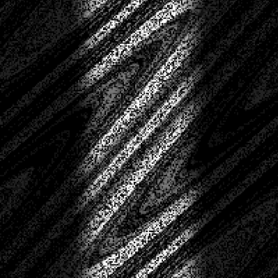
FIG. 4.: Predator 2d pattern obtained for $p=0.37$. The distribution of nutrients is continuous. The lighter the colour the higher the concentration.

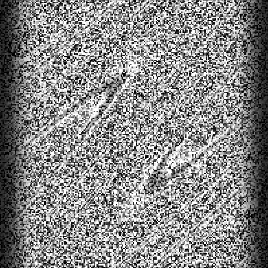
FIG. 5.: Predator 2d pattern obtained for $p=0.87$. The distribution of nutrients is continuous.

REFERENCES

- [1] E.R. Abraham, The generation of plankton patchiness by turbulent stirring, Nature, 391, 577-580 (1998).
- [2] M.J.R. Fasham, The statistical and mathematical analysis of plankton patchiness, Oceanogr. Mar. Biol. Ann. Rev., 16, 43 (1978).
- [3] J.H. Steele, ed., Spatial patterns in plankton communities, Plenum Press, New York NY, 1978.
- [4] J.H. Steele and E.W. Henderson, Coupling between physical and biological scales, Phil. Trans. R. Soc. Lond. B, 343, 5 (1994).
- [5] L. Mazzella, M.C. Buia, M.C. Gambi, M. Lorenti, G.F. Russo, M.B. Scipione, V. Zupo, Plant-animal trohic relationships in the Posidonia Oceanica ecosystem of the Mediterranean Sea: a review, in: D.M. John, S.J. Hawkins and J.H. Price (eds) Plant-animal interactions in the marine benthos, Clarendon Press, Oxford, 165, 1992.
- [6] I.R. Jenkinson, and B.A. Biddanda, Bulk-phase viscoelastic properties of seawater: relationship with plankton components, Journal of Plankton Research, 17, 2251-2274 (1995).
- [7] I.R. Jenkinson, T. Wyatt, and A. Malej, How viscoelastic effects of colloidal biopolymers modify rheological properties of seawater, Progress and Trends in Rheology 5, 57, 1998.
- [8] J.M. Ottino, The kinematics of mixing: stretching, chaos and transport, Cambridge University Press, Cambridge, 1989.
- [9] J.H.E. Cartwright, M. Feingold, and O. Piro, An introduction to chaotic advection in Mixing: Chaos and Turbulence, H. Chaté, E. Villermaux, and J.-M. Chomaz, eds. (Kluwer Academic/Plenum Publishers, New York, 1999).
- [10] J.H.E. Cartwright, M. Feingold, and O. Piro, Passive scalars and three-dimensional Liouvillian maps, Physica D 76, 22-33 (1994).
- [11] A.J. Lichtenberg and M.A. Lieberman, Regular and Chaotic Dynamics, Springer-Verlag, New York, 1992.
- [12] V. Loreto, G. Paladin, M. Pasquini, and A. Vulpiani, Characterization of chaos in random maps, Physica A 232, 189 (1996).
- [13] C.-H. Lai, Changsong Zhou, Synchronization of Chaotic Maps by Symmetric Common Noise, Europhys. Lett. 43, 376 (1998).
- [14] R. Toral, C.R. Mirasso, E. Hernández-García, and O. Piro Synchronization of Chaotic Systems by Common Random Forcing in Unsolved Problems of Noise and Fluctuations: UPON’99, Second international conference. D. Abbot, L. Kish, editors (AIP, Melville, 2000).
- [15] Z. Neufeld, C. López, and P.H. Haynes, Smooth-filamental transition of active tracer fields stirred by chaotic advection, Phys. Rev. Lett., 82, 2606 (1999).
- [16] Z. Neufeld, C. López, E. Hernández-García, and T. Tél, The multifractal structure of chaotically advected chemical fields, Phys. Rev. E, 61, 3857 (2000)
- [17] C. Canuto, M. Y. Hussaini, A. Quarteroni and T. A. Zang, Spectral methods in fluid dynamics (Springer-Verlag, New York, 1988).