Function and form in networks of interacting agents

Abstract

The main problem we address in this paper is whether function determines form when a society of agents organizes itself for some purpose or whether the organizing method is more important than the functionality in determining the structure of the ensemble.

As an example, we use a neural network that learns the same function by two different learning methods. For sufficiently large networks, very different structures may indeed be obtained for the same functionality. Clustering, characteristic path length and hierarchy are structural differences, which in turn have implications on the robustness and adaptability of the networks.

In networks, as opposed to simple graphs, the connections between the agents are not necessarily symmetric and may have positive or negative signs. New characteristic coefficients are introduced to characterize this richer connectivity structure.

Keywords: networks, agents, clustering, path length.

1 Introduction

Networks of interacting agents play an important modelling role in fields as diverse as computer science, biology, ecology, economy and sociology. An important notion in these networks is the distance between two agents. Depending on the circumstances, distance may be measured by the strength of interaction between the agents, by their spatial distance or by some other criterium expressing the existence of a link between the agents. Based on this notion, global parameters have been constructed to characterize the connectivity structure of the networks. Two of them are the clustering coefficient and the characteristic path length. The clustering coefficient measures the average probability that two agents, having a common neighbor, are themselves connected. The characteristic path length is the average length of the shortest path connecting each pair of agents. These coefficients are sufficient to distinguish randomly connected networks from ordered networks and from small world networks. In ordered networks, the agents being connected as in a crystal lattice, clustering is high and the characteristic path length is large too. In randomly connected networks, clustering and path length are low, whereas in small world networks[1] [2] [3] clustering may be high while the path length is kept at a low level.

An important question is to find out what the mechanisms are, that lead to each type of structure, when a network of interacting agents evolves in time. In general, networks of agents organize themselves for some purpose. For example, a country is organized to insure the survival and well-being of its inhabitants (or of a subset thereof, anyway), supply networks are organized to bring food to a town every day and the network of neurons in the brain is organized to process the information that arrives through the sensorial organs. Therefore one might be led to think that it is the function of the network that determines its form. A simple example shows that it is not necessarily so. Restaurants and private homes in a large city do not keep more than a few days worth of food and without a continuous replenishment of their reserves the city would collapse in a few days. The supply problem of several million inhabitants is solved every day in most cities by a self-organized network of producers, transporters and retailers where clustering and a short path length are the rule. Alternatively, in a centralized economy, a different, very structured system may be organized with producers delivering their goods to a local cooperative, where they are collected by a state-organized transportation agency, which then delivers it to a few centralized stores, where all consumers are supposed to acquire their goods. In this case one has a very regular structure. People might say that one system is more efficient than the other, but that is quite irrelevant as far as functionality is concerned. In both cases the city is supplied and the fact is, that the structure of the two networks is quite different.

That institutions used in different societies to achieve similar aims may be very different is a well known fact. This also casts considerable doubt on any attempts to characterize the uniqueness of optimal solutions. The solutions that are arrived at must be largely history-dependent. Any optimality criterium should therefore not be based on the functionality of the solution, but on other factors like stability, resistance to change, adaptability to a changing environment, etc.

Of course, if there is only one possible configuration of the network for each desired functionality then, whenever the functionality is achieved, the form is fixed. In that case function determines form and the form does not dependent on the method by which the functionality is achieved. However, this is not the most frequent situation in networks of many agents. What we call the function of the network is associated to a few collective variables, like survival of the group, making war on a neighboring country, maintaining a few simple myths, extracting global concepts like color or pain from a multitude of external stimuli, etc. That is, the function of the network is related to a number of variables much smaller than the number of agents or internal degrees of freedom of the network. In that case it is to be expected that several distinct configurations of the network will be associated to the same functionality.

In the space of all the configurations that realize a given function, an important question is to know what types of network structures do exist, concerning in particular their connectivity properties (clustering, path length, etc.). This is the main problem we address in this paper. Because general statements about networks tend to be vague and do not go a long way, we concentrate in neural network models that are learning to represent a given function. The use of neural networks as a paradigm for networks of interacting agents is not so restrictive as it may seem because, as shown by Doyne Farmer[5], they are largely equivalent to many other connectionist systems. The distance between the agents (nodes) in the network is defined by the inverse of the absolute value of the connection strength. Nodes are considered to be connected if the connection strength exceeds a certain threshold. This threshold is not fixed a priori, but is determined by a clustering algorithm as the lowest value that insures connectivity of the whole network.

Two learning methods for the same function are tested and, using the distance defined by the connection strengths, clustering coefficients and characteristic path lengths are computed. The general conclusion is that, in fact, function does not determine form, very different structures being obtained (on average) by the two methods. The first learning algorithm is in the class of reinforcement learning methods, of which several variants exist[7] [8], whereas, in the second, the agents (nodes) are punished by mistakes but nothing happens when the answer is the desired one[9]. We will denote the first method by reinforcement learning method (RLM) and the second by learning from mistakes (LFM).

The neural network, as a network of agents, is richer than the graphs that, in the past, have been used to study connectivity in networks. This arises from the fact that not only the connections between nodes may be positive (excitatory) or negative (inhibitory), but also the connections are in general asymmetric, one node having an influence over other node different from the influence it receives from the latter. To characterize this additional information on the structure of the network we have introduced new quantities to measure these properties, namely symmetry, cooperation, antagonism and residuality coefficients as well as directed path lengths.

2 Clustering and path length in goal-oriented networks

As a paradigm for goal-oriented networks, we study a neural network which starts as randomly connected (with small connection strengths) and learns to reproduce a function by two different learning methods. A certain number of nodes are defined to be input nodes and some others output nodes. In the numerical experiments we report here, we have taken two nodes as input, one as output and the function to be reproduced is a Boolean function like the exclusive OR, for example. Similar results are obtained for other more complex functions. The only care to be taken is that the network should have a sufficiently large number of nodes to guarantee that the subspace of strength connections, compatible with implementation of that function, is large. Otherwise, if there is only one possible configuration of connection strengths, function determines form and the dependence on the learning method cannot be detected. It is also obvious that, even when the regions in function space, explored by different learning methods, are distinct, it may happen that, by chance, configurations obtained by different methods do coincide. This is borne out in our experiments, some overlap being observed between the configurations obtained by different learning methods. However, on average, different methods explore quite different regions of the function space.

The results we obtain, indicate that the structures resulting from the reinforcement learning method (RLM) exhibit a high clustering coefficient together with an intermediate value for the characteristic path length. On the other hand, the structures obtained by the learning from mistakes method (LFM) have a low clustering coefficient with characteristic path lengths similar to those obtained from random structures, that is, similar to the structures used to initialize the network. RLM seems to be largely dependent on the establishment of a highly clustered configuration while LFM does not require the creation of such an ordered structure. One may think of the structures created by the latter method as being those of a highly adaptive system where specific tasks are performed without strongly committed configurations.

2.1 The network and the learning algorithms

The network we study is characterized by a non-layered architecture representing a fully connected system of twelve agents with connection strengths initially chosen at random in the interval $-0.5<w_{ij}<0.5$.

The absolute value of the connection strength $w_{ij}$ corresponds to the inverse distance of the agent pair $i$,$j$. From the initial, random, configuration, two different learning algorithms were used to obtain an XOR function. The first one is a Hebbian-like method, while the second relies on the learning from mistakes approach, with reinforcement being replaced by a process of depressing the synaptic connections involved in mistakes[9]. Both have a biological inspiration, the first one corresponding to long term synaptic potentiation[7] and the second to long term synaptic depression[10].

In both learning methods, a sigmoid function $\phi$ is used as activation function and the computation of the output signal includes a bias $\alpha$, which operates as a regulatory mechanism for the overall activity of the network. If the network activity is too low, the bias $\alpha$ is decreased until an appropriate number of firing neurons is obtained. On the other hand, if the activity exceeds a certain limit, $\alpha$ is increased in order to keep a low level of activity in the network. A neuron is defined as firing if its output is above $50\%$ of the maximum output ($1$).

Reinforcement learning method (RLM)

The connections between firing neurons are strengthened or weakened according to whether the output is successful or not. The process affects all firing neurons in the same way. The reinforcement updating rule is:

If the output is the correct one

$$w_{ij}:=w_{ij}+(\delta Y_{i}Y_{j})$$

otherwise

$$w_{ij}:=w_{ij}-(\delta Y_{i}Y_{j})$$

$Y_{i}=\phi\left(\sum_{k}w_{ik}Y_{k}\right)$ is the output of neuron $i$ and $\delta<<1$.

Also, as stated before, the bias is adjusted to keep the overall network activity at a low level. Saturation is avoided by a global rescaling of all the coupling strengths, when one of them exceeds a fixed threshold.

Learning from mistakes (LFM)

If the output happens to be the desired one, nothing is done, otherwise the connections between firing neurons are depressed by a fixed amount $\delta$, which is redistributed among the connections between non-firing neurons,

$$w_{ij}:=w_{ij}-\delta$$

with $\delta<<1$

As in RLM, there is a global regulatory mechanism to keep the overall activity at a low level.

2.2 Clustering coefficient and characteristic path length

Clustering coefficient (CC) and characteristic path length (CPL) are important statistical parameters used in graph theory. These two parameters have been the object of growing attention ever since the small-world phenomenon was identified as an interesting property of the structures found in many different fields. The small-world feature[3] is characteristic of structures with CC similar to the one obtained in regular structures but with CPL’s close to those of random networks.

In the past, graph modelling concerned itself mostly with completely random or completely regular structures. Regular graphs combine high CC with large CPL while, in the opposite case, random graphs exhibit low CC and small CPL. Starting from a completely regular structure and applying a random rewiring procedure to interpolate between regular and random networks it has been found[2] that there is a broad interval of structures over which CPL is almost as small as in random graphs and yet CC is much greater than expected in the random case. This rewiring procedure helps to characterize the structural aspects of a network in the transition from order to disorder.

In the work presented here, the networks move in the opposite direction, from completely random towards a goal-oriented structure. The basic intuition is that forcing a randomly weighted network to learn a function by different learning methods, may lead to different forms of organization even though the methods are both targeted at reaching the same functional goal. In particular, we want to find out to what extent the success of a learning method is dependent on the transition from disorder to order in the network structure. The connectivity of the (starting) randomly connected networks provides reference values that help to characterize the lack of order. In the other extreme, the more regular structures that arise from learning are evaluated by finding out how much their CC and CPL differ from those that characterize randomness in the starting configurations.

CC and the CPL usually apply to graph structures that are connected and sparse. Since the networks we work with are fully-connected structures, a first step is targeted at obtaining a sparse representation of the network, with the degree of sparseness generated by the learning method itself, instead of an a priori specification. Notice that, when looking for a suitable degree of sparseness, one must avoid disconnected graphs (where the value of the CPL of any disconnected element would be infinite). For this purpose we construct of a graph structure from the connection strengths.

The graph representation of the network

From the $n\times n$ matrix $W$ of connection strengths, $\left\{w_{ij}\right\}$, we construct a $n\times n$ distance matrix $D_{W}$, with elements $d_{ij}=\mid 1/w_{ij}\mid$. Based on the distances $d_{ij}\in D_{W}$, a hierarchical clustering is then performed using the nearest neighbor method. Initially $n$ clusters corresponding to the $n$ agents are considered. Then, at each step, two clusters $c_{i}$ and $c_{j}$ are clumped into a single cluster if

$$d_{c_{i}c_{j}}=\min\left\{d_{c_{i}c_{j}}\right\}$$

with the distance between clusters being defined by

$$d_{c_{i}c_{j}}=\min\left\{d_{pq}\right\}$$

with $p\in c_{i}$ and $q\in c_{j}$

This process is continued until there is a single cluster. This clustering process is also known as the single link method, being the method by which one obtains the minimal spanning tree (MST) of a graph. In a connected graph, the MST is a tree of $n-1$ edges that minimizes the sum of the edge distances.

In a network with $n$ agents, the hierarchical clustering process takes $n-1$ steps to be completed, and uses, at each step, a particular distance $d_{ij}\in D_{W}$ to clump two clusters into a single one. Let $C_{W}=\{d_{q}\}$, $q=1,...,n-1$, be the set of distances $d_{ij}\in D_{W}$ used at each step of the clustering, and $L_{W}=\max\{d_{q}\}$. It follows that $L_{W}=d_{n-1}$.

At this point we are able to define a representation of $D_{W}$ with sparseness replacing fully-connectivity in a suitable way. For this purpose, a boolean graph $B_{W}$ (with $n$ vertices being the network nodes) is defined setting $b_{ij}=1$ if $d_{ij}\leq L_{W}$ and $b_{ij}=0$ if $d_{ij}>L_{W}$. As usual, null arcs of $B_{W}$ are those for which $b_{ij}=0$ while for unit arcs $b_{ij}=1$. Here we want to consider two nodes $i$ and $j$ to be connected if either $d_{ij}$ or $d_{ji}\leq L_{W}$ . Therefore we take $b_{ij}=\max\{b_{ij},b_{ji}\}$. Later on (Sect. 3) we will take into account directional effects.

Let $A_{W}$ be the matrix associated with $B_{W}$. Each element $a_{ij}$ is the number of edges of $B_{W}$ that join the vertices $i$ and $j$ and, since $B_{W}$ is a simple graph, $a_{ij}\in\{0,1\}$.

The degree of $B_{W}$, or its coordination number $k$, represents the average number of unit arcs leaving each element of the graph. The coordination number characterizes the sparseness of the graph and has an important bearing on its properties[3]. In our approach we obtain the value of $k$ from the network itself. Therefore we avoid any a priori estimation and, by the hierarchical clustering method, we also avoid disconnectivity.

We are also interested in defining $C_{W}^{*}=\{d_{l}\}$, $l=1,...,m$, as the set of distances $d_{ij}\in D_{W}$ whose values are less or equal to $L_{W}$, and computing $r=m-(n-1)$. Clearly $r\geq 0$ is the number of redundant elements in $C_{W}^{*}$, that is, the number of distances $d_{ij}$ that, although being smaller than $L_{W}$, need not be considered in the hierarchical clustering process. Later on, we will discuss the relation between the value of $r$ and the clustering coefficient of the graph.

Clustering coefficient

The clustering coefficient (CC) of a graph $G$ (averaged over all vertices $v$ of $G$) measures whether two vertices adjacent to another vertex $v$ are adjacent to each other. When CC=1 one has a group of disconnected but individually complete subgraphs, while CC=0 implies that no neighbor of any vertex $v$ is adjacent to any other neighbor of $v$.

At the end of the learning process, we build an adjacency list from the matrix $A_{W}$ associated with $B_{W}$. It is done by listing all vertices of $B_{W}$ and, next to each one, its neighboring vertices. From the adjacency list of $B_{W}$ the clustering coefficient of $B_{W}$ may be found in two different ways.

1. The first method computes the value of the clustering coefficient $CC_{v}$ of each vertex $v$ by dividing the number of unit arcs in the neighborhood of $v$ by the total number of arcs in such a neighborhood, which is given by $s_{v}(s_{v}-1)/2$, $s_{v}$ being the size of the adjacency list of vertex $v$. Averaging over all vertices of $B_{W}$ we obtain a coefficient which we denote by $CA_{B_{W}}$.

2. In the second method the calculation of the clustering of $B_{W}$ does not consider the vertices $v$ of $G$ that have just one vertex in its neighborhood. For each pair of unit arcs $(v_{1},v_{2})$ and $(v_{2},v_{3})$ of $B_{W}$ that share a common vertex $v_{2}$ we count one if $(v_{1},v_{3})$ corresponds to a unit arc, otherwise we count nothing. The total sum is then divided by

   $$\sum_{v=1}^{n}s_{v}(s_{v}-1)/2$$

   where $s_{v}$ is the size of the adjacency list of each vertex $v$ of $B_{W}$. In this way, vertices with a single vertex in its neighborhood do not contribute to the value computed by the above expression (since $s_{v}-1=0$), being those vertices consequently excluded from the computation of $CC_{B_{W}}$.

Notice that, for a typical network, the values of $CC_{B_{W}}$ and $CA_{B_{W}}$ tend to be very similar. A significant difference between these values indicates either that the network has many single-neighbor vertices ($CC_{B_{W}}>CA_{B_{W}}$) or that the distribution of the clustering coefficients for each vertex is very heterogeneous ($CC_{B_{W}}<CA_{B_{W}}$). To control these effects we have, for our simulations, computed both $CA_{B_{W}}$ and $CC_{B_{W}}$.

Above, we have defined $C_{W}^{*}=\left\{d_{l}\right\}$ $\left(l=1,...,m\right)$ as the set of distances $d_{ij}\in D_{W}$ with values less or equal to $L_{W}$ and $r=m-(n-1)$ as the number of redundant elements in $C_{W}^{*}$, that is, the number of distances $d_{ij}$ that, although being smaller than $L_{W}$, are not used in the hierarchical clustering process.

In a connected graph $r$ provides the cardinality of the cycle basis of $B_{W}$, or its cyclomatic number. Being a cycle basis of a graph defined by the set of its elementary cycles that taken together yield the entire graph, itself a cycle. In the next section, when discussing the simulation results, we notice that, depending on the learning method, cycles and trees (i.e., connected graphs without cycles) may or not appear in the resulting network structures. The clustered networks have a high coordination number while in the opposite case the networks approach a tree-like structure and, consequently, a low clustering coefficient.

Characteristic path length

The characteristic path length (CPL) of a weighted graph is the average length of the shortest path between any two vertices in the graph. From the $n\times n$ matrix $W$ of connection strengths, $\left\{w_{ij}\right\}$, and its corresponding distance matrix $D_{W}$, the weighted graph $G_{W}$ (with $n$ vertices corresponding to the network nodes) is defined by

$$g_{ij}=\min\{d_{ij},d_{ji}\}$$

We compute the characteristic path length of a weighted graph $G_{W}$, by taking for each pair $(i,j)$ in $G_{W}$, with $i\neq j$, the smallest distance $spl(i,j)$ between $i$ and $j$. The $n(n-1)/2$ edges $g_{ij}$ are sequentially taken from a list where the $g_{ij}$ were sorted in ascending order. In the first step, the smallest $g_{ij}$ in the list provides the shortest distance between $i$ and $j$. In the next steps, the new edge $g_{e_{1}e_{2}}$ provides the shortest $spl(e_{1},e_{2})$ distance between $e_{1}$ and $e_{2}$ and may also provide another smallest path length by $spl(i,j)+spl(e_{1},e_{2})$ if $e_{1}$ or $e_{2}\in\{i,j\}$, namely:

$$\begin{array}[]{l}\textnormal{if }i=e_{1}\hskip 8.5359ptspl(e_{2},j)=\min\{spl(e_{2},j),spl(e_{2},e_{1})+spl(i,j)\}\\ \textnormal{if }i=e_{2}\hskip 8.5359ptspl(e_{1},j)=\min\{spl(e_{1},j),spl(e_{2},e_{1})+spl(i,j)\}\\ \textnormal{if }j=e_{1}\hskip 8.5359ptspl(e_{2},i)=\min\{spl(e_{2},i),spl(e_{2},e_{1})+spl(i,j)\}\\ \textnormal{if }j=e_{2}\hskip 8.5359ptspl(e_{1},i)=\min\{spl(e_{1},i),spl(e_{2},e_{1})+spl(i,j)\}\end{array}$$

In the following steps we check whether the edge being considered, composed with the previously established minimal paths, defines a path $spl^{*}(i,j)$ that is smallest than a previously computed $spl(i,j)$. If it happens $spl^{*}(i,j)$ replaces $spl(i,j)$.

This computation is sequentially repeated until the shortest distance $spl(i,j)$ between each pair of nodes in the graph is obtained. Averaging over the $n(n-1)/2$ edges of $G_{W}$, we obtain the CPL of $G_{W}$.

Results

The results presented here were obtained from several simulations in networks which start as randomly connected. A typical random network is shown in Fig. 1. In this figure, the absolute value of each connection strength ($w_{ij}$) of the network specifies the grey intensity of the corresponding patch in the image. White patches represent null connections (null arcs). Units 1 and 2 are taken to be inputs and unit 12 is the output. This is the reason why the other units do not connect back to 1 and 2 and unit 12 does not connect back to the others.

The absolute values of the connection strengths corresponding to the inverse of distances, dark patches represent small distances. With connection strengths chosen in the interval $-0.5<w_{ij}<0.5$, an almost black patch means $d_{ij}\sim 0$, while an white patch corresponds to $\mid d_{ij}\mid\sim$ 0.5.

Figure 1: A typical random network

The connectivity of random networks provides reference values to characterize the goal-oriented structures that are obtained by the learning methods. For this purpose, Fig. 2 shows the image of the adjacency matrix of a typical random network. It was obtained by:

1. Taking the network structure represented in Fig.1

2. Applying the hierarchical clustering process to obtain the distance $d_{n-1}\in C_{W}$ used in the last step of hierarchical clustering

3. Building the corresponding boolean graph with adjacency matrix shown in Fig. 2. Unit arcs ($d_{ij}\leq d_{n-1}$) are represented as black patches while null arcs ($d_{ij}>d_{n-1}$) correspond to white ones.

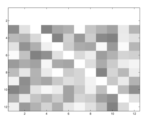
Figure 2: Adjacency matrix of a typical random network

As shown in Fig. 2, the graphs that represent the random structures used to initialize the network are characterized by a high degree of sparseness (a small number of black patches in the corresponding image). The degree $k$ of the graph is much smaller than the number of agents in the network. Moreover, in these graphs the number of unit arcs $u$ is usually only slightly larger than $n-1$, which is the minimum value that ensures connectivity. As a consequence, the number of redundant elements in the graph is small and the graph approaches a tree-like structure, with a small clustering coefficient (see table 1).

Fig. 3 shows the typical final structure of a network that starts as randomly connected and is organized by learning from mistakes (LFM). The image shows that LFM networks are similar to the typical random structure shown in Fig. 1. The distribution of connection strengths is not, in general, very different from those generated at random, suggesting that LFM does not require the creation of a very organized structure in order to reach its functional goal.

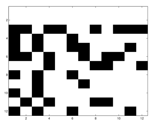
Figure 3: Typical LFM network

The image shown in Fig. 4 was obtained following the same steps as used for the image in Fig. 2. It is built from the network shown in Fig.3. It represents the adjacency matrix of a typical LFM network. Given that the typical LFM structures differ little from a random configuration, it exhibits a significant degree of sparseness. Looking at Fig. 4 we see that the number of unit arcs ($u$) remains close to $n-1$, hence the number of redundant elements in the graph is almost as small as in random networks. In a significant number of simulations, the final structures are even closer to tree-like structures, with a consequently low clustering coefficient.

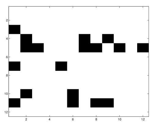
Figure 4: Adjacency matrix of a typical LFM network

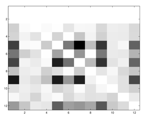
Figure 5: Typical RLM network

Fig. 5 shows a typical configuration for a network that learned through RLM. Small and large distances are not so well distributed as they were at random, showing that RLM networks move away from the initial configuration in order to reach its functional goal. The degree of sparseness of Fig. 6 confirms this fact. The degree of sparseness of a typical RLM structure is smaller than that of a random one and also smaller than the degree of sparseness of a typical LFM network. Some of the connection intensities are strongly increased during the learning process and the final network very often presents a significant degree of symmetry.

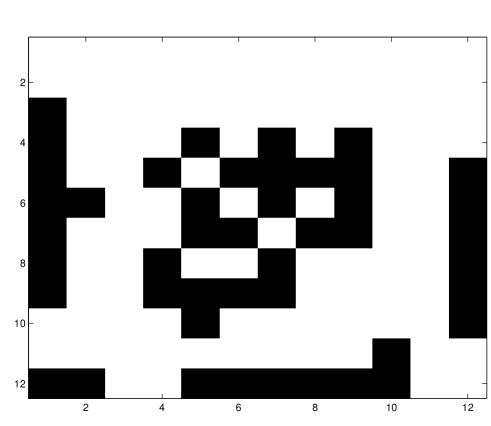
Figure 6: Adjacency matrix of a typical RLM network

The number of black patches strongly increases in the structure represented in Fig. 6 showing that the number of unit arcs ($u$) is much greater than $n-1$. Consequently, the number of redundant elements in the graph is significantly greater than in random networks. As shown in this figure, the final RLM structures tend to contain cycles and move away from the tree-like structures that appear in random and LFM networks.

Table 1 shows typical values for the degree of the graphs ($k$),the clustering coefficient (CC and CA) and the characteristic path length (CPL) for random, LFM and RLM networks. In each case we show the mean (x̄) and the standard deviation ($\sigma_{x}$) obtained in the simulations.

	$\overline{CC}$	$\sigma_{CC}$	$\overline{CA}$	$\sigma_{CA}$	$\overline{CPL}$	$\sigma_{CPL}$	$\bar{k}$	$\sigma_{k}$
Rand	0.26	0.16	0.24	0.17	1.6	0.05	3.3	1.0
LFM	0.25	0.15	0.35	0.20	2.1	0.2	3.0	0.69
RLM	0.57	0.19	0.53	0.16	5.6	1.16	4.5	1.3

Table 1: k, CC and CPL typical values

Figs. 7 and 8 show the distributions of the clustering coefficient and the characteristic path length for random, LFM and RLM networks. As mentioned in the introduction, even though the regions in function space explored by different learning methods are distinct, it happens that, by chance, configurations obtained by different methods may coincide.

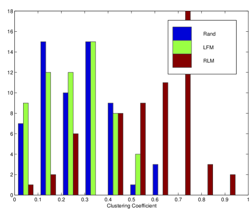
Figure 7: Custering coefficient distribution

The histograms of both CPL and CC confirm that there is some overlap between the configurations obtained by different learning methods. However, on average, as far as clustering and characteristic path length are concerned, LFM and RLM exhibit quite different structures.

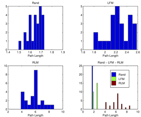
Figure 8: Characteristic path length distribution

On the other hand, as far as these parameters are concerned, LFM networks have structures similar to random networks.

3 Directional network coefficients

The coefficients introduced in this section aim at characterizing the richer connectivity structure of the learning networks because the strengths of interaction between agents (and their corresponding spatial distances) are not necessarily symmetric and may have positive or negative signs.

3.1 Directed path length

The directed path length (DPL) of a weighted graph provides the average length of the shortest directed path between any two vertices in the graph. In order to compute the directed path length of a network we take the $n\times n$ matrix $W$ of connection strengths, $\left\{w_{ij}\right\}$, and its corresponding distance matrix $D_{W}$, $d_{ij}=\mid 1/w_{ij}\mid$. The weighted and directed graph $dG_{W}$ is defined by setting

$$dg_{ij}=d_{ij}$$

As in the computation of the characteristic path length, the ($n(n-1)-2$) edges are sequentially taken from a list with the $dg_{ij}$ sorted in ascending order. In the first step, the smallest $dg_{ij}$ in the list provides the shortest distance between $i$ and $j$. In the following steps, each new edge in the list plays a double role: $dg_{e_{1}e_{2}}$ provides a distance $dpl(e_{1},e_{2})$ between $e_{1}$ and $e_{2}$ by $dpl(e_{1},e_{2})=g_{e_{1}e_{2}}$ and it may also provide a smaller distance $dpl(e_{1},j)$ or $dpl(i,e_{2})$ whenever $e_{1}=j$ or $e_{2}=i$. Namely,

$$\begin{array}[]{l}\textnormal{if }i=e_{2}\hskip 8.5359ptdpl(e_{1},j)=\min\{dpl(e_{1},j),dpl(e_{1},e_{2})+dpl(i,j)\}\\ \textnormal{if }j=e_{1}\hskip 8.5359ptdpl(i,e_{2})=\min\{dpl(i,e_{2}),dpl(e_{1},e_{2})+dpl(i,j)\}\end{array}$$

At each step one checks whether the edge being considered defines a path $dpl^{*}(i,j)$ that is smaller than a previously computed $dpl(i,j)$. If it happens $dpl^{*}(i,j)$ replaces $dpl(i,j)$.

This computation is sequentially repeated until all the $n*(n-1)-2$ edges in the list are considered. In so doing, the smallest distance $dpl(i,j)$ between all pairs of nodes in the graph is obtained. Averaging over the $n(n-1)-2$ edges of $dG_{W}$, we obtain the DPL of $dG_{W}$.

Results

Figs. 9 shows the distributions of the directed path length for random, LFM and RLM networks.

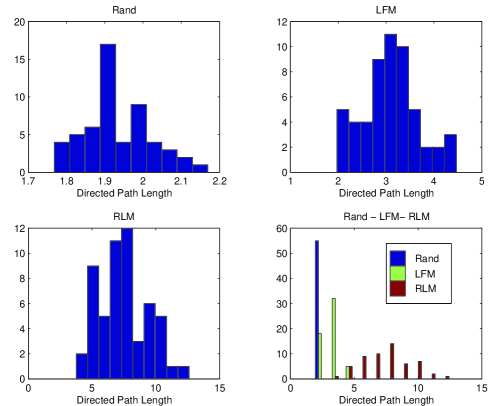
Figure 9: Directed path length distribution

Table 2 shows typical values for the degree of the graphs ($k$) and the directed path length (DPL) for random, LFM and RLM networks. In each case we show the mean (x̄) and the standard deviation ($\sigma_{x}$) obtained in the simulations.

	$\overline{DPL}$	$\sigma_{DPL}$	$\bar{k}$	$\sigma_{k}$
Rand	2.1	0.7	3.3	1.0
LFM	3.0	2.3	3.0	0.69
RLM	7.5	5.6	4.5	1.3

Table 2: $k$ and DPL typical values

When the orientation of the edges is taken into account, the average length of the shortest path in random, LFM and RLM networks naturally increases. The results show that the three types of networks exhibit a similar increase as compared to the previously obtained CPL values (see table 1). It is still between random and LFM networks that we find closer values. The typical RLM networks have a higher DPL, showing that, when the directions of the edges are considered, a RLM network still exhibits properties that characterize structures away from randomness. It is in accordance with the idea that the success of its underlying method is much more dependent on the acquisition of an ordered structure than the learning by mistakes method.

3.2 Symmetry, cooperation, antagonism and residuality coefficients

As opposed to simple graphs, the connections between the agents in the networks that we have been studying (and in most natural occurring networks) are not symmetric and may have positive or negative signs. It is therefore convenient to be able to characterize this richer connectivity structure. For this purpose some new coefficients are defined. A symmetry coefficient ($S$) is defined by

$$S=1-\sum_{i>j}^{n}\mid w(i,j)-w(j,i)\mid/\sum_{i>j}^{n}max(\mid w(i,j)\mid,\mid w(j,i)\mid)$$

It follows that $-1\leq S\leq 1$. From the value of $S$ we are able to evaluate how far the learning networks are from a perfectly symmetric structure $(S=1)$ and which learning method contributes more to changing the values $(S\sim 0.5)$ that characterize a typical random network. The results in table 3 show that on average, after learning, the symmetry coefficient increases both for RLM and LFM networks. As far as symmetry is concerned, the two methods behave similarly.

In addition we may also define cooperation ($C$), and antagonism ($A$) coefficients by

$$C=\sum_{w(i,j)>0}^{n}w(i,j)/\sum_{i\neq j}^{n}\mid w(i,j)\mid$$

$$A=-(\sum_{w(i,j)<0}^{n}w(i,j)/\sum_{i\neq j}^{n}\mid w(i,j)\mid)$$

with $C+A=1$.

Initially, the networks are initialized at random in the interval $-0.5<w_{ij}<0.5$. The randomly chosen connections tend to be uniformly distributed between positive and negative strengths $(C\sim A\sim 0.5)$. One may think of the positive connection strengths as representing cooperation between agents, while the negative ones represent antagonistic interactions. The highest degree of cooperation (and the lowest of antagonism), corresponding to $C=1$ (and $A=0$), is reached when every network connection has a positive sign. Conversely the lowest degree of cooperation ($C=0$, $A=1$) is characteristic of a network where every connection strength is negative.

The last coefficient we will define is the residuality ($R$) coefficient

$$R=\sum_{1/\left|w(i,j)\right|>L_{W}}\mid w(i,j)\mid/\sum_{1/\left|w(i,j)\right|\leq L_{W}}\mid w(i,j)\mid$$

where $L_{W}$ is the highest threshold distance value $\left|1/w(i,j)\right|$ that insures connectivity of the whole network in the hierarchical clustering process of Sect. 2.1. Residuality relates the relative strengths of the connections above and below the threshold value.

Table 3 shows the average values obtained for the symmetry (S), cooperation (C), antagonism (A) and residuality (R) coefficients in random, LFM and RLM networks.

	$S$	$C$	$A$	$R$
Rand	0.57	0.51	0.49	2.6
LFM	0.70	0.94	0.05	1.8
RLM	0.75	0.66	0.33	0.6

Table 3: Symmetry, cooperation, antagonism and residuality

The results show that, before learning, in the random networks the weight of the connections below the threshold $1/L_{W}$ is two to three times higher than the weight of the connections above the threshold. After learning the residuality coefficient decreases in both the LFM and RLM networks, with a very significant decrease in the RLM networks. This is due to the fact that RLM networks become less sparse after learning (see $\bar{k}$ in table 2) forcing several residual connections to leave this category. For the LFM networks, although sparseness does not change much after learning, the decrease of $R$ happens because, the connection strengths above $1/L_{W}$ tend to be stronger than those that remain below the threshold.

Cooperation (and antagonism) behaves quite differently depending on the learning method. In LFM networks, $C$ approaches $1$ after learning, while, in a typical RLM network, the value of the cooperation coefficient stays around $2/3$. Antagonism seems to disappear on LFM learning. On the other hand, RLM learning keeps a reasonable degree of antagonism $(A=0.33)$ in the network structure.

4 Robustness and adaptability

The networks we have studied acquire a structure while learning a function. While clustering and path length bring information on the connectivity of the structures, the characterization of the mechanisms leading to each type of structure raises a few other questions, namely:

(i) How easily will the acquired structure adapt itself to the representation of another function?

(ii) To what extent do the structures succeed in keeping the same functionality when some of their connections are suppressed?

As a first step to answer these questions we have measured the adaptability of RLM and LFM networks as follows:

1. A network with connection strengths chosen at random in the interval $-0.5<w_{ij}<0.5$, learns to reproduce the exclusive OR function

2. After learning the matrix $x_{ij}$ keeps the resulting normalized $\left(x_{ij}=w_{ij}/max(w_{ij})\right)$ connection strengths

3. The network with connection strengths $x_{ij}$ learns to reproduce the AND function

4. After learning we obtain the matrix $a_{ij}$ of the resulting normalized connection strengths

5. The network adaptability coefficient $\gamma_{N}$ is computed by

   $$\gamma_{N}=\sum_{i,j=1}^{n}\mid x_{ij}-a_{ij}\mid$$

Averaging $\gamma$ over the results of several simulations we have obtained $\overline{\gamma}_{LFM}=30.8$, yields an average change $\Delta x_{ij}=0.25$ when LFM is the method that is chosen.

Following the same set of steps as above in order to compute the adaptability of RLM networks turns out to be quite difficult because step 3 frequently fails. In contrasts with LFM structures, adaptation in RLM networks is almost absent and new learning is efficient only if one starts from scratch, i.e., from a randomly connected network structure.

These results indicate that the configurations obtained by different learning methods behave quite differently as far as adaptability is concerned. The structures created by the LFM method are those of a highly adaptive system whereas for RLM the structures that are created seem to become highly specialized for its purpose.

To evaluate the robustness of the structures the following algorithm is applied:

(i) A vector $\left\{x_{i}\right\}$ of $n(n-1)$ components is defined, corresponding each components to a particular connection in the network. The vector is initialized with zeros.

(ii) After the learning process, one cuts each one of the connections in turn and tests whether the learned function is still reproduced. If the test fails one adds a one to the corresponding component of the vector $\left\{x_{i}\right\}$.

(iii) The test is repeated for all the connections and for a certain number of different networks (60 different networks in our simulations)

(iv) The distribution $P(x)$ of the values stored in the vector $\left\{x_{i}\right\}$ is plotted.

Figs. 10 and 11 show the results corresponding to LFM and RLM networks with the same number of trials in each case.

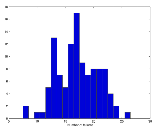
Figure 10: Distribution of failures for LFM networks

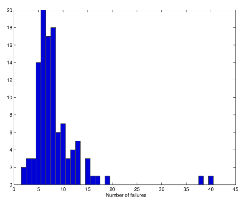
Figure 11: Distribution of failures for RLM networks

The results indicate that RLM networks are more robust than those resulting from the LFM method. The former exhibit, on average, a smaller number of errors, suggesting that, individually, the role of any specific connection is less important for reaching the desired functionality than in RLM networks. Moreover, in the case of RLM networks the distribution of failures (Fig. 11) shows that some connections are much more important than others (those that contribute to the fat tail), while a large amount of connections play a smaller role.

5 Conclusions

In multi-agent networks the overall functionality or collective behavior does not uniquely determine the interaction topology and the graph structure of the network. This happens because, in general, many different configurations are associated to the same (small number) of relevant collective variables. Then, the organizing method, that is, the evolution history of the network, is the main determining factor on the establishment of a particular type of structure on the network. These general conclusions are borne out by our study of networks that, starting from a random configuration, learn to represent a function by two different learning methods.

Clustering coefficients and (non-directed) characteristic path lengths turn out to be appropriate to discriminate the two organizing methods that were used. In particular, a striking confirmation of the ”function does not determine form” assertion is obtained from the fact that the high clustering and intermediate path length of RLM networks indicate that reinforcement learning establishes a highly ordered configuration, whereas the same functionality is obtained in LFM networks with low clustering and path lengths similar to random networks.

The idea that learning something or reaching some goal requires some degree of order is well accepted. So is the knowledge that regular structures - in opposition to those generated at random - exhibit high clustering and large path length. Recent work has shown that there is a multitude of cases where the structures of interest lie in a broad interval between regular and random. In this paper we have shown that there are cases where the same goal may be achieved by structures near both extremes. Achieving a goal does not necessarily require very organized structures. Moreover when the method followed to achieve the goal implies the establishment of a high degree of order, the resulting structures tend to be hard to adapt to any different goal. As shown in the last section of the paper, algorithms may be developed to characterize, in a quantitive manner, the degree of robustness and adaptability of the networks.

In the neural-like networks that we have been using (and in most natural occurring networks) the interactions between the agents are not symmetric and may have positive or negative signs. This in contrast to the simple graph structures used in the past to study interaction topologies. Directed path lengths, as well as symmetry, cooperation, antagonism and residuality coefficients were defined, which provide a refined characterization of the network structures. Relevant differences were also found between the learning methods when these new coefficients are measured. For example, starting from a random network, LFM seems to strongly improve cooperation, whereas in RLM cooperation increases only slightly.

References

- [1] J. W. Clark, G. C. Littlewort and J. Rafelski; Topology, structure and distance in quasirandom neural networks in Computer simulation in brain science, R. M. J. Cotterill (Ed.) Cambridge Univ. Press, Cambridge 1988.
- [2] D. J. Watts and S. H. Strogatz; Collective dynamics of small-world networks, Nature 393 (1998) 440-442.
- [3] D. J. Watts; Small Worlds, Princeton Univ. Press, Princeton 1999.
- [4] F. Albertini and E. D. Sontag; For neural networks, function determines form, Neural Networks 6 (1993) 975 - 990.
- [5] J. Doyne Farmer; A Rosetta stone for connectionism, Physica D 42 (1990) 153 - 187.
- [6] J. S. Denker, D. B. Schwartz, B. S. Winter, S. A. Solla, R. E. Howard, L. D. Jackel and J. J. Hopfield; Large automatic learning, rule extraction and generalization, Complex Systems 1 (1987) 877 - 922.
- [7] D. O. Hebb; The organisation of behaviour, Wiley, New York 1949.
- [8] D. Stassinopoulos and P. Bak; Democratic reinforcement: a principle for brain function, Phys. Rev. E51 (1995) 5033–5039.
- [9] Dante R.Chialvo and Per Bak; Learning from mistakes, adap-org/9707006.
- [10] F. Crepel, N. Hemart, D. Jaillard and H. Daniel; Long term depression in the cerebellum, in The Handbook of Brain Theory and Neural Networks, M. A. Arbib (Ed.), MIT Press, Cambridge 1995.