Fronts in passive scalar turbulence

Abstract

The evolution of scalar fields transported by turbulent flow is characterized by the presence of fronts, which rule the small-scale statistics of scalar fluctuations. With the aid of numerical simulations, it is shown that : isotropy is not recovered, in the classical sense, at small scales; scaling exponents are universal with respect to the scalar injection mechanisms ; high-order exponents saturate to a constant value ; non-mature fronts dominate the statistics of intense fluctuations. Results on the statistics inside the “plateaux”, where fluctuations are weak, are also presented. Finally, we analyze the statistics of scalar dissipation and scalar fluxes.

]

I Introduction

The understanding of small-scale fluctuations in scalar fields, such as temperature, pollutant density, chemical or biological species concentration, advected by turbulent flow is of great interest in both theoretical and practical domains [1]. Propagation phenomena of light beams and radio waves in the atmosphere are for example strongly influenced both by the magnitude and the spatial distribution of small-scale temperature gradients [2]. Their dynamical properties have been a subject of very accurate experimental investigations carried out in the last few years both in the atmosphere [2, 3], in the ocean [4, 5] and for laboratory turbulent flow [6, 7, 8, 9]. A striking feature of all these situations is the presence of fronts (also called sheets or cliffs). The important point is that the scalar field has very strong variations across the fronts, separated by large regions (“ramps” or “plateaux”) where scalar fluctuations are weak (see for example Fig. 17).

In the atmosphere, “ramp-and-cliff” structures in the temperature field extend from the ground to the middle stratosphere [2]. They are of major importance for the ubiquitous stratospheric radar echoes [10] and the problem of their formation is known as frontogenesis [11]. For the temperature field it is crucial to take into account its active nature, i.e. the fact that it influences the advecting velocity field. Simplified quasi and/or semi-geostrophic models have been proposed and investigated for the frontogenesis and we refer the interested reader to Refs. [11, 12] and references therein.

Cliffs such as those observed in the active case have in fact been observed also for passive situations, i.e. when the scalar field does not affect the advecting velocity field. Remarkably, cliffs are not mere footprints of velocity structures and they arise both for velocity fields that are solutions of the Navier–Stokes (NS) equations [13, 14] and for synthetic velocity fields [15, 16, 17, 18], including when the velocity is rapidly varying in time (the so-called Kraichnan case [19]). As emphasized in Refs. [13, 15, 20], the velocity gradient stretching is weak in the elliptic regions of the velocity field, where their ‘rotational’ character inhibits the formation of strong scalar gradients. Conversely, compressions along specific directions take place in the hyperbolic regions of the incompressible flow, scalar particles coming from distant regions of space approach each other and strong scalar gradients are thus developed.

The observation of ramp-and-cliff structures naturally raises the issue of their consequences for the scalar statistical properties and their possible implications for models of scalar transport. Two points will be specifically addressed here for the passive scalar case. Part of the results were previously summarized in Ref. [14].

The first concerns the role of ramps and cliffs for the scalar anisotropy. A central postulate of the classical Kolmogorov–Obukhov–Corrsin theory (see, e.g., Ref. [21]) for passive scalar turbulence is that the anisotropy degree should decay as smaller and smaller scales are considered. When the system is driven by an anisotropic forcing, such as a large-scale scalar gradient, the most common experimental situation, isotropy is usually supposed to be fully recovered at small scales. However, the evidence stemming from the experiments is that this is not the case (at least not in the original sense, see the following). Ramps and cliffs are preferentially aligned with the direction of the large-scale scalar gradient and this permits the anisotropies to find their way down to the smallest excited scales. In particular, the probability density function (pdf) for the scalar derivatives along the direction of the large-scale scalar gradient are strongly skewed. Furthermore, the scalar gradient skewness (that should vanish for an isotropic field) is $O(1)$, independently of the Péclet number [6, 7, 8, 9, 13, 15]. This leads us to investigate scalar turbulence universality, i.e. its degree of independence of injection mechanisms.

Recent numerical and experimental works exploiting symmetries under rotations point to the fact that anisotropic turbulent fluctuations are subdominant with respect to isotropic ones. We shall discuss the relation between these results and the aforementioned experimental observations about the persistence of large-scale anisotropies.

The second issue associated to the presence of cliffs concerns their role for the statistics of scalar difference strong fluctuations, i.e. to the behavior of high-order structure functions. In particular, scalar variations across the cliffs are comparable to the root-mean-square (rms) value of the scalar. This suggests that scalar structure function scaling exponents might saturate, that is tend to a constant for large enough orders. The question of saturation was first raised in Ref. [19]. Here, we shall provide evidence for saturation in two different situations : scalar advection by a two-dimensional Navier–Stokes velocity field in the inverse cascade regime and in the three-dimensional Kraichnan model [19]. As discussed in the sequel, the latter model represents the least favorable case to observe saturation, because of the velocity short correlation time. The fact that saturation is still observed points to the genericity of the phenomenon for scalar turbulence.

The paper is organized as follows. In Sections  II and  III, we recall some well-known results about the expected classical laws for the decay of anisotropies in scalar turbulence and the properties of the Navier-Stokes two-dimensional inverse energy cascade, respectively. Anisotropies and scalar turbulence universality are discussed in Section IV, while the results about saturation are presented in Section V. The successive Section investigates ramp-and-cliff structure dynamical processes. The aim is to clarify whether the observed saturation arises from ‘mature’ cliffs, having thicknesses comparable to the dissipative scale, or from ‘non-mature’ ones, still in the process of steepening. Section VII reports results on the scalar statistics inside the “plateaux”. Scalar dissipation is the subject of Section VIII, and the results on scalar fluxes, involving joint velocity-scalar correlations, are discussed in Section IX. The last Section is devoted to conclusions.

II The classical theory of scalar turbulence

The advection-diffusion partial differential equation governing the evolution of a passive scalar field $T(\mathchoice{{\hbox{\boldmath$\displaystyle r$}}}{{\hbox{\boldmath$\textstyle r$}}}{{\hbox{\boldmath$\scriptstyle r$}}}{{\hbox{\boldmath$\scriptscriptstyle r$}}},t)$ is :

$$\partial_{t}T(\mathchoice{{\hbox{\boldmath$\displaystyle r$}}}{{\hbox{\boldmath$\textstyle r$}}}{{\hbox{\boldmath$\scriptstyle r$}}}{{\hbox{\boldmath$\scriptscriptstyle r$}}},t)+\mathchoice{{\hbox{\boldmath$\displaystyle v$}}}{{\hbox{\boldmath$\textstyle v$}}}{{\hbox{\boldmath$\scriptstyle v$}}}{{\hbox{\boldmath$\scriptscriptstyle v$}}}(\mathchoice{{\hbox{\boldmath$\displaystyle r$}}}{{\hbox{\boldmath$\textstyle r$}}}{{\hbox{\boldmath$\scriptstyle r$}}}{{\hbox{\boldmath$\scriptscriptstyle r$}}},t)\cdot\nabla\,T(\mathchoice{{\hbox{\boldmath$\displaystyle r$}}}{{\hbox{\boldmath$\textstyle r$}}}{{\hbox{\boldmath$\scriptstyle r$}}}{{\hbox{\boldmath$\scriptscriptstyle r$}}},t)=\kappa\Delta T(\mathchoice{{\hbox{\boldmath$\displaystyle r$}}}{{\hbox{\boldmath$\textstyle r$}}}{{\hbox{\boldmath$\scriptstyle r$}}}{{\hbox{\boldmath$\scriptscriptstyle r$}}},t).$$ (1)

Here, $\mathchoice{{\hbox{\boldmath$\displaystyle v$}}}{{\hbox{\boldmath$\textstyle v$}}}{{\hbox{\boldmath$\scriptstyle v$}}}{{\hbox{\boldmath$\scriptscriptstyle v$}}}(\mathchoice{{\hbox{\boldmath$\displaystyle r$}}}{{\hbox{\boldmath$\textstyle r$}}}{{\hbox{\boldmath$\scriptstyle r$}}}{{\hbox{\boldmath$\scriptscriptstyle r$}}},t)$ is the incompressible advecting velocity field and $\kappa$ is the molecular diffusivity. The “energy” $T^{2}$ is statistically conserved by the advection term in (1) and dissipated by the viscous term. In order to attain a stationary state it is thus necessary to inject scalar fluctuations. The simplest way is to add a forcing term $f(\mathchoice{{\hbox{\boldmath$\displaystyle r$}}}{{\hbox{\boldmath$\textstyle r$}}}{{\hbox{\boldmath$\scriptstyle r$}}}{{\hbox{\boldmath$\scriptscriptstyle r$}}},t)$ to the right-hand side (rhs) of (1). A convenient choice that we shall use in this work is to take the forcing $f$ random, Gaussian, statistically homogeneous, isotropic, white in time, of zero mean and correlation function

$$\langle f(\mathchoice{{\hbox{\boldmath$\displaystyle r$}}}{{\hbox{\boldmath$\textstyle r$}}}{{\hbox{\boldmath$\scriptstyle r$}}}{{\hbox{\boldmath$\scriptscriptstyle r$}}},t)\,f(\mathchoice{{\hbox{\boldmath$\displaystyle 0$}}}{{\hbox{\boldmath$\textstyle 0$}}}{{\hbox{\boldmath$\scriptstyle 0$}}}{{\hbox{\boldmath$\scriptscriptstyle 0$}}},0)\rangle=\chi\left(r/L_{f}\right)\,\delta(t).$$ (2)

The correlation $\chi\left(r/L_{f}\right)$ is concentrated at the forcing integral scale $L_{f}$ and rapidly decreases for $r\gg L_{f}$.
An alternative injection mechanism, closer to typical experimental situations, is to maintain a mean scalar gradient $\textstyle g$. Scalar fluctuations $\theta$ superimposed on it, $T(\mathchoice{{\hbox{\boldmath$\displaystyle r$}}}{{\hbox{\boldmath$\textstyle r$}}}{{\hbox{\boldmath$\scriptstyle r$}}}{{\hbox{\boldmath$\scriptscriptstyle r$}}},t)\equiv\theta(\mathchoice{{\hbox{\boldmath$\displaystyle r$}}}{{\hbox{\boldmath$\textstyle r$}}}{{\hbox{\boldmath$\scriptstyle r$}}}{{\hbox{\boldmath$\scriptscriptstyle r$}}},t)+\mathchoice{{\hbox{\boldmath$\displaystyle g$}}}{{\hbox{\boldmath$\textstyle g$}}}{{\hbox{\boldmath$\scriptstyle g$}}}{{\hbox{\boldmath$\scriptscriptstyle g$}}}\cdot\mathchoice{{\hbox{\boldmath$\displaystyle r$}}}{{\hbox{\boldmath$\textstyle r$}}}{{\hbox{\boldmath$\scriptstyle r$}}}{{\hbox{\boldmath$\scriptscriptstyle r$}}}$, obey the equation of motion :

$$\partial_{t}\theta(\mathchoice{{\hbox{\boldmath$\displaystyle r$}}}{{\hbox{\boldmath$\textstyle r$}}}{{\hbox{\boldmath$\scriptstyle r$}}}{{\hbox{\boldmath$\scriptscriptstyle r$}}},t)+\mathchoice{{\hbox{\boldmath$\displaystyle v$}}}{{\hbox{\boldmath$\textstyle v$}}}{{\hbox{\boldmath$\scriptstyle v$}}}{{\hbox{\boldmath$\scriptscriptstyle v$}}}(\mathchoice{{\hbox{\boldmath$\displaystyle r$}}}{{\hbox{\boldmath$\textstyle r$}}}{{\hbox{\boldmath$\scriptstyle r$}}}{{\hbox{\boldmath$\scriptscriptstyle r$}}},t)\cdot\nabla\,\theta(\mathchoice{{\hbox{\boldmath$\displaystyle r$}}}{{\hbox{\boldmath$\textstyle r$}}}{{\hbox{\boldmath$\scriptstyle r$}}}{{\hbox{\boldmath$\scriptscriptstyle r$}}},t)=\kappa\Delta\theta(\mathchoice{{\hbox{\boldmath$\displaystyle r$}}}{{\hbox{\boldmath$\textstyle r$}}}{{\hbox{\boldmath$\scriptstyle r$}}}{{\hbox{\boldmath$\scriptscriptstyle r$}}},t)-\mathchoice{{\hbox{\boldmath$\displaystyle g$}}}{{\hbox{\boldmath$\textstyle g$}}}{{\hbox{\boldmath$\scriptstyle g$}}}{{\hbox{\boldmath$\scriptscriptstyle g$}}}\cdot\mathchoice{{\hbox{\boldmath$\displaystyle v$}}}{{\hbox{\boldmath$\textstyle v$}}}{{\hbox{\boldmath$\scriptstyle v$}}}{{\hbox{\boldmath$\scriptscriptstyle v$}}}.$$ (3)

Note that the mean gradient injection mechanism selects by its very definition a preferential direction in the system and isotropy is thus broken.

We shall be interested in the passive scalar structure functions

$$S_{n}(\mathchoice{{\hbox{\boldmath$\displaystyle r$}}}{{\hbox{\boldmath$\textstyle r$}}}{{\hbox{\boldmath$\scriptstyle r$}}}{{\hbox{\boldmath$\scriptscriptstyle r$}}})\equiv\langle[T(\mathchoice{{\hbox{\boldmath$\displaystyle x$}}}{{\hbox{\boldmath$\textstyle x$}}}{{\hbox{\boldmath$\scriptstyle x$}}}{{\hbox{\boldmath$\scriptscriptstyle x$}}}+\mathchoice{{\hbox{\boldmath$\displaystyle r$}}}{{\hbox{\boldmath$\textstyle r$}}}{{\hbox{\boldmath$\scriptstyle r$}}}{{\hbox{\boldmath$\scriptscriptstyle r$}}},t)-T(\mathchoice{{\hbox{\boldmath$\displaystyle x$}}}{{\hbox{\boldmath$\textstyle x$}}}{{\hbox{\boldmath$\scriptstyle x$}}}{{\hbox{\boldmath$\scriptscriptstyle x$}}},t)]^{n}\rangle\equiv\langle\left(\delta_{r}T\right)^{n}\rangle,$$ (4)

where $\langle\,\rangle$ denotes the average over the velocity, and possibly the forcing, ensemble. The reason to focus on correlations of the field $T$ rather than those of the field $\theta$ is explained in Appendix A. Throughout this work we assume the velocity to be scale-invariant, at least in the scalar inertial range of scales defined by $\eta\ll|\mathchoice{{\hbox{\boldmath$\displaystyle r$}}}{{\hbox{\boldmath$\textstyle r$}}}{{\hbox{\boldmath$\scriptstyle r$}}}{{\hbox{\boldmath$\scriptscriptstyle r$}}}|\ll L$. Here, $\eta$ is the scalar dissipation scale and $L$ is the scalar integral scale. For the mean-gradient injection, $L$ is comparable to the velocity integral scale. For the randomly forced case, we shall consider situations where the velocity integral scale is comparable (or even larger) than the forcing one and therefore $L\simeq L_{f}$. On account of these assumptions, the scalar structure functions are expected to have a scaling behavior in the inertial range of scales. For the isotropic randomly forced case, odd orders vanish by symmetry. For the injection by a mean gradient, both even and odd-order structure functions are non-zero.

For even-order structure functions, the classical prediction of the Kolmogorov–Obukhov–Corrsin (KOC) theory is :

$$S_{2n}(r)=C_{2n}\epsilon_{\theta}^{n}\,\epsilon_{v}^{-n/3}r^{2n/3}\left({L\over r}\right)^{\rho_{n}}\propto r^{\zeta_{2n}},$$ (5)

with $\zeta_{2n}=2n/3$ and the anomaly $\rho_{2n}\equiv 2n/3-\zeta_{2n}=0$. In the previous formula, $\epsilon_{\theta}\equiv\kappa\langle(\nabla\theta)^{2}\rangle$ is the mean scalar energy dissipation, $C_{2n}$ are non-dimensional constants and the velocity is assumed to be of Kolmogorov-type, with velocity increments $\langle(\delta_{r}v)^{n}\rangle\propto r^{n/3}$ and a finite energy flux $\epsilon_{v}$. The same arguments can be reformulated along the same lines for other types of velocity fields.

Dimensional arguments are easily extended to odd-order moments in the presence of a mean gradient $\textstyle g$ [22]. The balance between the advection term and the injection term on the rhs of (3) gives indeed

$$S_{2n+1}(\mathchoice{{\hbox{\boldmath$\displaystyle r$}}}{{\hbox{\boldmath$\textstyle r$}}}{{\hbox{\boldmath$\scriptstyle r$}}}{{\hbox{\boldmath$\scriptscriptstyle r$}}})\sim\left(\mathchoice{{\hbox{\boldmath$\displaystyle g$}}}{{\hbox{\boldmath$\textstyle g$}}}{{\hbox{\boldmath$\scriptstyle g$}}}{{\hbox{\boldmath$\scriptscriptstyle g$}}}\cdot\mathchoice{{\hbox{\boldmath$\displaystyle r$}}}{{\hbox{\boldmath$\textstyle r$}}}{{\hbox{\boldmath$\scriptstyle r$}}}{{\hbox{\boldmath$\scriptscriptstyle r$}}}\right)S_{2n}(\mathchoice{{\hbox{\boldmath$\displaystyle r$}}}{{\hbox{\boldmath$\textstyle r$}}}{{\hbox{\boldmath$\scriptstyle r$}}}{{\hbox{\boldmath$\scriptscriptstyle r$}}})\propto r^{\zeta_{2n+1}},$$ (6)

with $\zeta_{2n+1}=2n/3+1$. The classical prediction for the decay rate of hyperskewnesses $R_{n}$ is then :

$$R_{n}\equiv\frac{S_{2n+1}}{S_{2}^{n+1/2}}\propto r^{2/3}\qquad n=1,2,\cdots$$ (7)

Predictions for the scaling of scalar gradient moments with the Péclet number are obtained by substituting $r=\eta\propto{\rm Pe}^{-3/4}$ in the structure function expressions (5) and (7). It follows in particular that, in the presence of a large-scale gradient $\textstyle g$, the skewness of the scalar gradient along this direction should decrease as ${\rm Pe}^{-1/2}$.

Notice that the classical KOC scalings do not explicitly involve the integral scale $L$. Anomalous scalings correspond to the violations of these behaviors, i.e. $\zeta_{n}\neq n/3$, and the appearance of the integral scale $L$ in the structure function expressions via the non-vanishing anomalies $\rho_{n}$.

III The advecting velocity fields

We discuss now the choice of the advecting velocity field in Eqs. (1) or (3). The flow that we shall consider mostly in this work is the one arising from a two-dimensional Navier–Stokes inverse energy cascade [23]. Its properties are briefly recalled in the following subsection. In order to corroborate the results on saturation, we shall also consider in Section V B three-dimensional synthetic flows of the Kraichnan type (see Refs. [19, 24]).

A The 2D Navier-Stokes flow

The two-dimensional Navier–Stokes equation for the vorticity $\omega(\mathchoice{{\hbox{\boldmath$\displaystyle r$}}}{{\hbox{\boldmath$\textstyle r$}}}{{\hbox{\boldmath$\scriptstyle r$}}}{{\hbox{\boldmath$\scriptscriptstyle r$}}},t)=-\Delta\psi(\mathchoice{{\hbox{\boldmath$\displaystyle r$}}}{{\hbox{\boldmath$\textstyle r$}}}{{\hbox{\boldmath$\scriptstyle r$}}}{{\hbox{\boldmath$\scriptscriptstyle r$}}},t)$ is :

$$\partial_{t}\omega+J\left(\omega,\psi\right)=\nu\Delta\omega-\alpha\omega-\Delta{\cal F},$$ (8)

where the velocity $\textstyle v$ is related to the stream function $\psi$ as $\mathchoice{{\hbox{\boldmath$\displaystyle v$}}}{{\hbox{\boldmath$\textstyle v$}}}{{\hbox{\boldmath$\scriptstyle v$}}}{{\hbox{\boldmath$\scriptscriptstyle v$}}}=\nabla^{\perp}\psi=(\nabla_{y}\psi,-\nabla_{x}\psi)$, the Jacobian is denoted by $J$ and the forcing by ${\cal F}$. The friction linear term $-\alpha\omega$ extracts energy from the system at scales comparable to the friction scale $\eta_{\rm fr}\sim\epsilon_{v}^{1/2}\alpha^{-3/2}$, assuming a Kolmogorov scaling law for the velocity. As before, $\epsilon_{v}$ indicates the mean energy dissipation.

Let us first recall from Ref. [25] some technical details on the numerical integration of (8). To focus on the inverse cascade phase and avoid the Bose-Einstein condensation in the gravest mode [23], we choose $\alpha$ to make $\eta_{\rm fr}$ sufficiently smaller than the box size. The other relevant length in the problem is the small-scale forcing correlation length $l_{\cal F}$, bounding the inertial range for the inverse cascade as $l_{\cal F}\ll r\ll\eta_{\rm fr}$. We use a Gaussian forcing with correlation function $\langle{\cal F}(\mathchoice{{\hbox{\boldmath$\displaystyle r$}}}{{\hbox{\boldmath$\textstyle r$}}}{{\hbox{\boldmath$\scriptstyle r$}}}{{\hbox{\boldmath$\scriptscriptstyle r$}}},t)\,{\cal F}(\mathchoice{{\hbox{\boldmath$\displaystyle 0$}}}{{\hbox{\boldmath$\textstyle 0$}}}{{\hbox{\boldmath$\scriptstyle 0$}}}{{\hbox{\boldmath$\scriptscriptstyle 0$}}},t^{\prime})\rangle=\delta(t-t^{\prime})\,F(r/l_{\cal F})$. The forcing correlation decays rapidly for $r\gg l_{\cal F}$ and we choose $F(x)=F_{0}l_{\cal F}^{2}\exp(-x^{2}/2)$, where $F_{0}$ is the energy injection rate. The integration is performed by a standard $2/3$-dealiased pseudospectral method on a doubly periodic square domain $2048\times 2048$. The viscous term in Eq. (8) has the role of removing the enstrophy at scales smaller than $l_{\cal F}$ and, as customary, it is numerically more convenient to substitute it by a hyperviscous term (of order eight in our simulations). Time evolution is implemented by a standard second-order Adams-Bashforth scheme. The integration is carried out for one hundred eddy turn-over times after both the velocity and the scalar fields have reached the stationary state.

The inverse nature of the energy cascade clearly emerges from the third-order longitudinal structure function $V^{(3)}_{\parallel}(r)\equiv\langle\left[\left(\mathchoice{{\hbox{\boldmath$\displaystyle v$}}}{{\hbox{\boldmath$\textstyle v$}}}{{\hbox{\boldmath$\scriptstyle v$}}}{{\hbox{\boldmath$\scriptscriptstyle v$}}}(\mathchoice{{\hbox{\boldmath$\displaystyle r$}}}{{\hbox{\boldmath$\textstyle r$}}}{{\hbox{\boldmath$\scriptstyle r$}}}{{\hbox{\boldmath$\scriptscriptstyle r$}}},t)-\mathchoice{{\hbox{\boldmath$\displaystyle v$}}}{{\hbox{\boldmath$\textstyle v$}}}{{\hbox{\boldmath$\scriptstyle v$}}}{{\hbox{\boldmath$\scriptscriptstyle v$}}}(\mathchoice{{\hbox{\boldmath$\displaystyle 0$}}}{{\hbox{\boldmath$\textstyle 0$}}}{{\hbox{\boldmath$\scriptstyle 0$}}}{{\hbox{\boldmath$\scriptscriptstyle 0$}}},t)\right)\cdot{\mathchoice{{\hbox{\boldmath$\displaystyle r$}}}{{\hbox{\boldmath$\textstyle r$}}}{{\hbox{\boldmath$\scriptstyle r$}}}{{\hbox{\boldmath$\scriptscriptstyle r$}}}/r}\right]^{3}\rangle$. In analogy with the $4/5$ law valid for the three-dimensional case (see, e.g., Ref. [26]), one can indeed easily derive from (8) the relation $V^{(3)}_{\parallel}(r)=3/2\epsilon_{v}r$, expressing the upward constant energy flux. The neat plateau at the positive value $3/2$ visible in Fig. 1 is a clear confirmation of the inverse energy cascade.

FIG. 1.: Compensated third order longitudinal structure function $V^{(3)}_{\parallel}(r)/(\epsilon_{v}r)$. The dotted line is the value $3/2$. The vertical scale is linear.

An important property of the flow that has emerged both from numerical simulations [27, 25] and experiments [28] is the absence of intermittency in the velocity increment statistics. No corrections to the Kolmogorov scaling $r^{n/3}$ for the $n$-th order velocity structure function can be measured. In Fig. 2 we show indeed that velocity increment pdf’s at different separations $r$ can all be collapsed rescaling the increment $\delta_{r}v$ by their variance $\langle(\delta_{r}v)^{2}\rangle^{1/2}\sim r^{1/3}$. Furthermore, deviations from a Gaussian are small (at least for fluctuations not very large) and this has been exploited to propose a theory for the observed absence of intermittency [29].

The important point to our purposes here is that the velocity field arising from the 2D inverse energy cascade is scale-invariant (no intermittency) of exponent $1/3$, isotropic and, mostly important, has realistic correlation times. Contrary to synthetic flows, like those in [15] or the Kraichnan ensemble used in Section V B, the correlation times are finite and free of any sweeping-related pathology. The anisotropic and intermittency properties of the scalar field that will be discussed in the sequel are therefore intrinsic of the advection-diffusion passive scalar dynamics and not mere footprints of the advecting velocity.

FIG. 2.: Pdf’s of velocity fluctuations rescaled by their variance, for five lengthscales within the inverse energy cascade range. The dashed line is the Gaussian probability density.

IV Anisotropy and universality

The classical picture of the anisotropy decay presented in Section II is contradicted by the experimental observations. Contrary to the expected ${\rm Pe}^{-1/2}$ behavior, the skewness of the scalar derivative along the large-scale gradient $\partial_{\|}\theta\equiv\mathchoice{{\hbox{\boldmath$\displaystyle g$}}}{{\hbox{\boldmath$\textstyle g$}}}{{\hbox{\boldmath$\scriptstyle g$}}}{{\hbox{\boldmath$\scriptscriptstyle g$}}}\cdot\nabla\theta/|\mathchoice{{\hbox{\boldmath$\displaystyle g$}}}{{\hbox{\boldmath$\textstyle g$}}}{{\hbox{\boldmath$\scriptstyle g$}}}{{\hbox{\boldmath$\scriptscriptstyle g$}}}|$ does not show any measurable dependence on the Péclet number [6, 7, 8, 9, 30]. The corresponding pdf ${\cal P}(\partial_{\|}\theta)$ is strongly asymmetric with a sharp maximum located at $-g$, signaling the mean gradient expulsion out of the plateaux regions. The same general picture is also valid for passive scalar fields advected by synthetic flows.

The fact that the memory of the large-scale injection conditions is not lost going toward small scales makes it necessary to have a better understanding of scalar turbulence universality. To investigate the degree and the type of dependence of scalar turbulence on the injection mechanisms we have performed two series of numerical experiments. The advecting velocity field in both series is the two-dimensional NS velocity discussed in Section III A. The major difference is in the injection mechanisms. As discussed in Section II, the first of them is isotropic (random forcing) and the second is anisotropic (by a mean gradients $\textstyle g$). The comparison between the two sets of results will permit a quantitative analysis of universality.

A Anisotropy

For the anisotropic injection by a mean gradient, the scalar structure functions $S_{n}(\mathchoice{{\hbox{\boldmath$\displaystyle r$}}}{{\hbox{\boldmath$\textstyle r$}}}{{\hbox{\boldmath$\scriptstyle r$}}}{{\hbox{\boldmath$\scriptscriptstyle r$}}})$ depend on both $r=|\mathchoice{{\hbox{\boldmath$\displaystyle r$}}}{{\hbox{\boldmath$\textstyle r$}}}{{\hbox{\boldmath$\scriptstyle r$}}}{{\hbox{\boldmath$\scriptscriptstyle r$}}}|$ and $\phi$, the angle between $\textstyle r$ and $\textstyle g$. The latter dependence is best dealt with by expanding $S_{n}(r,\phi)$ on a proper set of orthonormal functions $U^{(\mathchoice{{\hbox{\boldmath$\displaystyle l$}}}{{\hbox{\boldmath$\textstyle l$}}}{{\hbox{\boldmath$\scriptstyle l$}}}{{\hbox{\boldmath$\scriptscriptstyle l$}}})}(\phi)$ :

$$S_{n}(r,\phi)=\sum_{l}S^{(l)}_{n}(r)U^{(l)}(\phi).$$ (9)

The most natural basis is made of the set $\cos(l\,\phi)$, $\sin(l\,\phi)$. This is the two-dimensional version of the SO(d) representation group exploited in Refs. [31, 32] to analyze experimental and numerical turbulence data. The sine functions are in fact absent in the expansion (9), since the scalar field is statistically invariant under the transformation $\phi\mapsto-\phi$. Furthermore, as a result of their opposite symmetries with respect to the transformation $\mathchoice{{\hbox{\boldmath$\displaystyle r$}}}{{\hbox{\boldmath$\textstyle r$}}}{{\hbox{\boldmath$\scriptstyle r$}}}{{\hbox{\boldmath$\scriptscriptstyle r$}}}\mapsto-\mathchoice{{\hbox{\boldmath$\displaystyle r$}}}{{\hbox{\boldmath$\textstyle r$}}}{{\hbox{\boldmath$\scriptstyle r$}}}{{\hbox{\boldmath$\scriptscriptstyle r$}}}$ ($\phi\mapsto\phi+\pi$), even and odd orders are expanded as

$$S_{2n}(\mathchoice{{\hbox{\boldmath$\displaystyle r$}}}{{\hbox{\boldmath$\textstyle r$}}}{{\hbox{\boldmath$\scriptstyle r$}}}{{\hbox{\boldmath$\scriptscriptstyle r$}}})=\sum_{l=0}^{n}\,S_{2n}^{(2l)}\,(r)\,\cos\,(2\,l\phi)\,,$$ (10)

$$S_{2n+1}(\mathchoice{{\hbox{\boldmath$\displaystyle r$}}}{{\hbox{\boldmath$\textstyle r$}}}{{\hbox{\boldmath$\scriptstyle r$}}}{{\hbox{\boldmath$\scriptscriptstyle r$}}})=\sum_{l=0}^{n}\,S_{2n+1}^{(2l+1)}\,(r)\,\cos\,[(2l+1)\phi]\,.$$ (11)

Scaling behaviors $S_{n}^{(l)}(r)\propto r^{\zeta_{n}^{(l)}}$ are expected in the inertial range. The n-th order structure function is thus made of a power law superposition. It is expected that the various contributions are ordered according to their anisotropic degree, i.e. $\zeta^{(l)}_{n}$ increases with $l$ for a fixed $n$ [32].

To extract the leading contribution to the scaling of $S_{n}(\mathchoice{{\hbox{\boldmath$\displaystyle r$}}}{{\hbox{\boldmath$\textstyle r$}}}{{\hbox{\boldmath$\scriptstyle r$}}}{{\hbox{\boldmath$\scriptscriptstyle r$}}})$, it is sufficient to project on the lowest-order components as

$$S_{2n}^{(0)}(r)=\frac{1}{2\pi}\,\int_{0}^{2\pi}S_{2n}(r,\phi)\,d\phi,$$ (12)

$$S_{2n+1}^{(1)}(r)=\frac{1}{2\pi}\,\int_{0}^{2\pi}S_{2n+1}(r,\phi)\,\cos\phi\,d\phi.$$ (13)

The scaling behaviors presented hereafter have been obtained by performing such angular averages over a set of 80 snapshots equally spaced by about one turn-over time. We have also verified that the contributions arising from higher anisotropic sectors are subdominant as expected, i.e. that the exponents associated to

$$S_{n}^{(l)}(r)=\frac{1}{2\pi}\,\int_{0}^{2\pi}S_{n}(r,\phi)\,\cos(l\phi)\,d\phi\qquad l\geq 2\,,$$ (14)

are larger than those for $l=0$ or $l=1$. A precise measurement of the subdominant anisotropic scaling exponents is rather delicate due to the cancellations needed for their statistical convergence and we shall not dwell on this.

A remark on the projection procedure is in order. In numerical simulations, it is easy to perform angular averages such as (12) or (13). This is not generally the case for laboratory experiments where measuring the data for all possible directions $\phi$ might be problematic. It is then useful to note that the results obtained by using the projections (12) or (13) essentially coincide with those where only the first subleading contributions are eliminated. This filtering is much more economic as it can be performed by a single measurement along $\phi=\pi/4$ for even orders and $\phi=\pi/6$ for odd-order structure functions.

FIG. 3.: The 3rd and the 5th-order parallel structure functions for the injection by a mean gradient. In the inset, local scaling exponents $dS_{n}(r)/d\log r$. The measured exponents are $\zeta_{3}=1.25\pm 0.04$, $\zeta_{5}=1.38\pm 0.07$, with error bars estimated from rms fluctuations of local scaling exponents.

Let us now present the results concerning the anisotropy decay rate, measured by odd-order structure functions. In Fig. 3, we show the $3$-rd and the $5$-th order structure functions. Accordingly, the skewness and hyperskewness coefficients of scalar differences scale as

$$S_{3}/S_{2}^{3/2}\sim r^{0.25},\qquad S_{5}/S_{2}^{5/2}\sim r^{-0.2},$$ (15)

the second-order scaling exponent being compatible, within the error bars, with the dimensional value $\simeq 2/3$ (see Fig. 7). Both behaviors (15) violate the dimensional prediction (7). Furthermore, whilst the skewness is decaying, even though much more slowly than the expected $r^{2/3}$, the hyperskewness grows at small scales. The effect of memory of the large-scale injection conditions observed in laboratory experiments is thus dramatically present also in our numerical simulations. The fact that clean scaling behaviors and exponents are measured here gives a very strong indication in favor of the fact that we are not dealing with a finite Péclet number effect. The most natural conclusion stemming from experiments, the previous and the present numerical simulations is that isotropy is not restored in the full classical sense, no matter how large is the Péclet number.

It is worth discussing in some more detail the relation between this last conclusion and the observation previously made on the subdominance of higher-order anisotropic contributions to structure functions. The problem comes of course from the presence of intermittency : contrary to the classical theory, the pdf of scalar differences ${\cal P}(\delta_{r}T)$ for various separations $r$ cannot be collapsed one onto another by a simple rescaling. Their change of shape with the separation $r$ makes it crucial to specify how the anisotropy degree is quantified and the amplitude of the fluctuations sampled in the pdf’s at various $r$’s. The ratio $S_{5}/S_{4}^{5/4}$ is for example decreasing with $r$, contrary to the hyperskewness in (15). The blow-up of the latter is thus a joined effect of anisotropy and intermittency. The point to be remarked is that odd-order structure functions are all scaling with exponents higher than those of structure functions of the same order but calculated with the absolute values, e.g. $\int|\delta_{r}T|^{3}\,{\cal P}(\delta_{r}T)\,d\delta_{r}T$. In other words, when fluctuations of similar amplitude are compared, anisotropic contributions are subdominant with respect to the isotropic ones. The same point is stressed in Fig. 4, where it is shown that the ratio between the anti-symmetric and the symmetric part of scalar increment pdf’s decreases with $r$. Notwithstanding the conclusion on the absence of isotropy restoration in the classical sense, it is thus important to realize that anisotropic fluctuations become more and more subdominant as their anisotropy degree increases.

FIG. 4.: Ratio between the anti-symmetric and the symmetric part of scalar increment pdf’s ${\cal P}(\delta_{r}T)$ for four separations in the inertial range.

B Universality

What is the degree of universality of scalar turbulence with respect to the injection mechanisms? Is the persistence of anisotropy just discussed signalling that the scalar statistics is totally imprinted by the non-universal large-scale injection conditions even at the smallest scales? To answer these questions it is convenient to compare observables, such as even-order structure functions or pdf’s themselves, that are meaningful and non trivial for both types of injection.

Let us first start from the scalar field pdf. Even though this is not a small-scale quantity, it is interesting that the two curves are different and the one for the mean-gradient injection is subgaussian, see Fig. 5. Note that this is not in contradiction with the exponential behavior predicted in [33, 41, 34]. The latter work considers indeed the situation where the velocity correlation length is much smaller than the typical length of variation of the large-scale mean scalar profile. In our case, these two lengths are of the order of the velocity friction length scale, defined in Section III, and of the box size, respectively. They are thus comparable. Similar subgaussian behaviors were also observed in [35].

FIG. 5.: The Pdf’s of the scalar field normalized by its standard deviation for the two cases of random forcing (upper curve, multiplied by a factor $10^{2}$ for plotting purposes) and injection by a mean gradient (lower curve). Note the presence of subgaussian tails for the latter (Gaussian densities are shown for comparison as dotted lines).

Let us move then to the small-scale statistics by considering scalar increments. In Fig. 6, we present the probability density functions for the two injection mechanisms : it is clear that they do not have the same shape and the same conclusion holds if we take only the symmetric part of the pdf’s. A particular consequence is that structure functions cannot have a universal expression, as postulated in the classical theory. It is however directly checked from Fig. 7 that the scaling exponents are the same for the two types of injection. This implies that the pdf’s, although having different shapes, rescale with $r$ in the same way.

FIG. 6.: Pdf’s of scalar increments normalized by their standard deviations for three separations $r=2.5\times\,10^{-2}$, $5\times\,10^{-2}$, $10^{-1}$ in the inertial range.

The scaling exponents being universal, the dependence on the large-scale injection conditions shows up in the structure function dominant expression $S_{n}(r)=C_{n}\epsilon_{\theta}^{n/2}\epsilon_{v}^{-n/6}r^{n/3}(L/r)^{n/3-\zeta_{n}}$ via the non-dimensional constants $C_{n}$. The resulting picture of universality is the following : structure function scaling exponents are independent of the injection details and thus universal ; scalar and scalar increment pdf’s, and non-dimensional constants in the structure functions are not. A particular instance is the one of odd-order structure functions, where the coefficients $C_{2n+1}$ vanish or not, depending on the symmetries of the injection mechanisms. This form of universality is weaker than the one in the original classical KOC theory and agrees with the remark made by L.D. Landau about the universality in Kolmogorov 1941 theory for fully developed turbulence. Remark finally that this universality framework is the same as the one arising from the zero mechanism in the Kraichnan passive scalar model [36, 37, 38].

FIG. 7.: Low-order even structure functions. Local scaling exponents are shown in the inset. The measured exponents are $\zeta_{2}=0.66\pm 0.03$, $\zeta_{4}=0.95\pm 0.04$ and $\zeta_{6}=1.11\pm 0.04$.

V Saturation of intermittency

The cliffs observed in scalar fields are strikingly suggestive of quasi-discontinuities. When smaller and smaller molecular diffusivities are considered, the minimal width of the fronts shrinks with the dissipation scale, with their maximum amplitude remaining comparable to the scalar rms value. Simple phenomenology suggests that the presence of such structures, corresponding to a local Hölder exponent equal to zero, might induce a vanishing slope in the structure function scaling exponent curve. The fronts being the strongest possible events, this behavior should take place for large enough orders, whence the possible saturation $\zeta_{n}\to{\rm const}$ for high $n$’s.

The first and most natural way to investigate the saturation is to look directly at the scalar structure function scaling exponents. An alternative procedure consists in looking, for a fixed $\delta_{r}T$, at how the pdf ${\cal P}(\delta_{r}T)$ of the scalar differences varies with the separation $r$. The latter is statistically more reliable than the former as less sensitive to the extreme tails of the pdf. Saturation is equivalent to the pdf taking the form

$${\cal P}(\delta_{r}T)=r^{\zeta_{\infty}}{\cal Q}\left(\frac{\delta_{r}T}{T_{rms}}\right)\frac{1}{T_{rms}},$$ (16)

for values of $\delta_{r}T\gtrsim T_{rms}\equiv\left(\langle T^{2}\rangle-\langle T\rangle^{2}\right)^{1/2}$. The tails of the (non-universal) ${\cal Q}$ function are bounded by the single-point scalar pdf, as it follows from the simple inequality (see, e.g., Ref. [39])

$$Prob\,\{|\delta_{r}T|>\tau\}\leq 2\,Prob\,\{|T|>\tau/2\}.$$ (17)

Both procedures have been used for the case of the Navier-Stokes advecting velocity field, where we could efficiently use spectral numerical methods. They present the disadvantage of being sensitive to finite-size effects but the advantage of giving access to the whole field and thus to the pdf’s. For the Kraichnan model, spectral methods are not very efficient and it is more convenient to use Lagrangian techniques (see Ref. [51, 40] for a detailed discussion). The latter permit very precise measurements of the scaling exponents at the price of not giving access to the pdf’s.

A Saturation with the Navier–Stokes advecting flow

The behaviors of the structure functions $S_{10}$, $S_{12}$ and $S_{14}$ in the presence of a large-scale scalar gradient are shown in Fig. 8. The scaling exponents $\zeta_{n}$ vs the order $n$ (up to the order $14$) are reported in Fig. 9. The curve is compatible with a saturation exponent $\zeta_{\infty}\sim 1.4$. The convergence of the moments was inspected by the usual test of checking whether $(\delta_{r}T)^{14}{\cal P}(\delta_{r}T)$ decays before the pdf ${\cal P}$ becomes noisy. The bulk contribution to the moments $10,12$ and $14$ is shown in Fig. 10. As for the second procedure on the pdf’s, following (16) we plot in Fig. 11 the curves $r^{-\zeta_{\infty}}{\cal P}(\delta_{r}T)$. Their collapse is a signature of the saturation and gives the unknown function ${\cal Q}$.

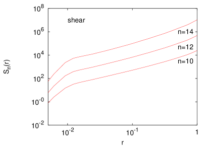
FIG. 8.: Scalar structure functions of orders $10,12$ and $14$ for the anisotropic injection mechanism

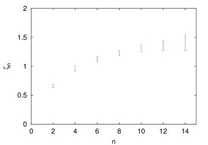
FIG. 9.: Measured scaling exponent $\zeta_{n}$ for the Navier–Stokes advection. Error bars are estimated by the rms fluctuations of local scaling exponents.

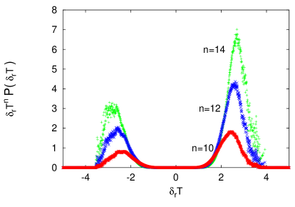
FIG. 10.: Bulk contribution to the $n$-th moment, $\delta_{r}T^{n}\cal P(\delta_{r}T)$, for $n=10,12,14$. Here $r$ is at the lower end of the inertial range.

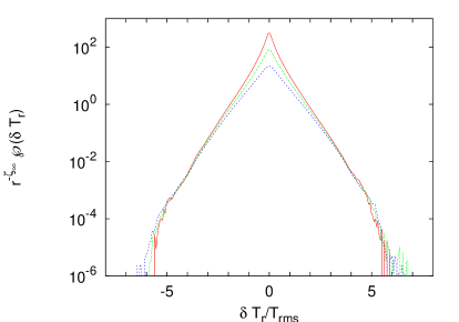
FIG. 11.: The pdf’s ${\cal P}(\delta_{r}T)$ , for the random forced injection, for three values of $r$ inside the inertial range of scales, multiplied by the factor $r^{-\zeta_{\infty}}$. The collapse of the curves indicates the presence of saturation and also gives the unknown function ${\cal Q}(\delta_{r}T/T_{rms})$ in Eq. (16).

In Fig. 12 we show the probabilities $\int_{\lambda\;T_{rms}}^{\infty}{\cal P}$ vs $r$ of having $\delta_{r}T>\lambda T_{rms}$ for various values of $\lambda$. The parallelism of the curves is again the footprint of saturation. Explicit evidence for the universality of $\zeta_{\infty}$ is provided in Fig. 13, where the probabilities $\int_{2.5\;T_{rms}}^{\infty}{\cal P}$ of having $\delta_{r}T>2.5\,T_{rms}$ are shown both for the isotropic and the non-isotropic injection mechanisms.

FIG. 12.: Probabilities $\int_{\lambda T_{rms}}^{\infty}{\cal P}$ vs $r$ of having $\delta_{r}T>\lambda T_{rms}$ for various $\lambda$. In the inside zoom, such probabilities are compensated by the factor $r^{-\zeta_{\infty}}$.

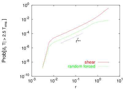
FIG. 13.: Probabilities $\int_{2.5\,T_{rms}}^{\infty}{\cal P}$ vs $r$ of having $\delta_{r}T>2.5T_{rms}$ for both the isotropic and non-isotropic injection mechanisms. The parallelism of the curves reflects the universality of the saturation exponent $\zeta_{\infty}$.

Both procedures give therefore a strong evidence in favor of saturation for the Navier-Stokes advecting velocity field.

B The case of the Kraichnan model

The advecting velocity field in the Kraichnan model [19] is assumed to be Gaussian, homogeneous, isotropic, of zero mean and correlation function

$$\langle\left(v(\mathchoice{{\hbox{\boldmath$\displaystyle r$}}}{{\hbox{\boldmath$\textstyle r$}}}{{\hbox{\boldmath$\scriptstyle r$}}}{{\hbox{\boldmath$\scriptscriptstyle r$}}},t)-v(\mathchoice{{\hbox{\boldmath$\displaystyle 0$}}}{{\hbox{\boldmath$\textstyle 0$}}}{{\hbox{\boldmath$\scriptstyle 0$}}}{{\hbox{\boldmath$\scriptscriptstyle 0$}}},t)\right)_{\alpha}\left(v(\mathchoice{{\hbox{\boldmath$\displaystyle r$}}}{{\hbox{\boldmath$\textstyle r$}}}{{\hbox{\boldmath$\scriptstyle r$}}}{{\hbox{\boldmath$\scriptscriptstyle r$}}},t)-v(\mathchoice{{\hbox{\boldmath$\displaystyle 0$}}}{{\hbox{\boldmath$\textstyle 0$}}}{{\hbox{\boldmath$\scriptstyle 0$}}}{{\hbox{\boldmath$\scriptscriptstyle 0$}}},t)\right)_{\beta}\rangle=$$ (18)

$$D\,r^{\xi}\left[(d+\xi-1)\delta_{\alpha\beta}-\xi{r_{\alpha}r_{\beta}\over r^{2}}\right],$$ (19)

where $d$ is the dimension of space. The assumption of $\delta$-correlation in time is of course far from the reality, but it has the remarkable feature of leading to closed equations for equal-time correlation functions $C_{n}\equiv\left\langle\theta(\mathchoice{{\hbox{\boldmath$\displaystyle r$}}}{{\hbox{\boldmath$\textstyle r$}}}{{\hbox{\boldmath$\scriptstyle r$}}}{{\hbox{\boldmath$\scriptscriptstyle r$}}}_{1},t)\ldots\theta(\mathchoice{{\hbox{\boldmath$\displaystyle r$}}}{{\hbox{\boldmath$\textstyle r$}}}{{\hbox{\boldmath$\scriptstyle r$}}}{{\hbox{\boldmath$\scriptscriptstyle r$}}}_{n},t)\right\rangle$ of any order $n$ (see, e.g., Refs. [24, 41]). This has permitted to rely the emergence of anomalous scaling and intermittency to the so-called zero modes, i.e. functions annihilated by the inertial operators appearing in the aforementioned closed equations  [36, 37, 38]. Anomalous zero modes can be calculated nonperturbatively for the case of a passively advected magnetic field [42] and for shell models à la Kraichnan [43]. For the case of the passive scalar, the expression for the second order correlation function $C_{2}$ is known exactly [24] and the inertial-range scaling behavior for the second-order structure function reads:

$$S_{2}(r;L)=\frac{2\chi(0)}{\zeta_{2}(d-1)dD}\,r^{\zeta_{2}}\qquad\zeta_{2}=2-\xi,$$ (20)

where $\chi(0)$, defined in (2), is the energy injection rate. The exponent $\zeta_{2}$ coincides with the predictions based on dimensional arguments and $\xi=4/3$ is the velocity exponent corresponding to the KOC scaling of the scalar field. Exact solutions are not available for higher orders and analytical predictions are perturbative in three different limits of the model : rough velocity fields $\xi\ll 1$ (Refs. [36, 44, 45]) ; large space dimensionalities $d\gg 1$ (Ref. [37]) and almost smooth velocity fields $\xi\to 2$ (Ref. [38]). In all of them, the order $n$ of the structure functions enters into the correction to the dimensional scaling together with the small parameter of the expansion. This means that, for any non-vanishing value of the expansion parameter, the predictions for $\zeta_{n}$ will break down at large enough $n$ and the very strong events associated to the extreme tails of the pdf’s cannot be captured by such procedures. To deal with the rare fluctuations responsible for the asymptotic behavior of the exponents $\zeta_{n}$ at large $n$’s, instantonic approaches have been borrowed from field theory [46, 47]. In the limit of very high $d$’s, the problem could be solved [48], with saturation taking place for $n\geq n^{*}$ (the latter diverging as $d\to\infty$). In the three-dimensional case, saturation has been phenomenologically suggested in Ref. [49] and inferred from an instantonic bound in Ref. [50].

Since numerical simulations are a fortiori limited to the measure of finite-order structure functions, it is important to choose the most convenient conditions to observe saturation. In particular, we expect that, for a fixed dimensionality of space, the orders where saturation takes place reduce with $\zeta_{2}=2-\xi$. This is due to the mechanism of cliff steepening. The latter is clearly favored by the presence of large-scale velocity components, inducing a coherent shear effect, and obstacled by small-scale velocity components, leading to effective diffusion effects. Since the amplitude of the former increases as $2-\xi$ reduces, we expect that saturation is favored by choosing $\xi$ close to two. Approaching too closely the Batchelor limit $\xi=2$ is however problematic from a numerical point of view, due to the presence of strong nonlocal effects. The chosen trade-off is to consider the three cases $\xi=1.875$, $\xi=1.84$, $\xi=1.75$, in 3D. The exponents being universal, it is more convenient to consider the isotropic injection mechanism (2) and we shall look at the fourth and the sixth-order structure functions.

FIG. 14.: The measured scaling exponent $\zeta_{n}$’s joined by straight-lines. (a) $\xi=1.875$; (b) $\xi=1.84$ and (c) $\xi=1.75$.

A detailed description of the Lagrangian method can be found in Refs. [51, 40] and will not be reported here. We only remark the fact that it naturally allows to measure the scaling of the structure functions $S_{2n}(r;L)$ vs the integral scale $L$ of the forcing. Physically, this means that the injection rate of the passive scalar variance (which equals its dissipation rate) and the separation $r$ are kept fixed, while the integral scale $L$ is varied. Anomalies, that is deviations from dimensional scaling exponents, are therefore measured directly (see (5)) through the scaling dependence on $L$ of the structure functions.

The measured $\zeta_{n}$’s are shown in Fig. 14 for: (a) $\xi=1.875$, (b) $\xi=1.84$ and (c) $\xi=1.75$. (The error bars are estimated by the rms fluctuations of local scaling exponents over intervals of constant length $\log_{10}5$ in log-space.) The corresponding behaviors of $S_{6}$ vs the integral scale $L$ are shown in Fig. 15 for $\xi=1.875$, $\xi=1.84$ and $\xi=1.75$, respectively. The structure function $S_{4}$ for $\xi=1.875$ is shown in Fig. 16. Similar high quality scaling laws have been obtained for $\xi=1.84$ and $\xi=1.75$. Some remarks about Fig. 14 are worth. It follows from Hölder inequalities that the $\zeta_{n}$ curve for $n>6$ must lie below the straight line joining $\zeta_{4}$ and $\zeta_{6}$. It seems unlikely that $\zeta_{n}$ can be a decreasing function of $n$. Indeed, an adaptation of the argument presented in Ref. [26], indicates that a decreasing $\zeta_{n}$ would entail arbitrarily large temperature differences at very small scales, something unphysical, given the maximum principle for the advection diffusion equation. Note that stricto sensu this argument applies only to the unforced equation, but the scalar scaling exponents are expected to be the same in the forced and in the unforced case (in its quasi-stationary phase). Hence, curve (a) in Fig. 14 and Hölder inequalities strongly constrain the behavior at higher $n$’s.

FIG. 15.: 3-d sixth order structure function $S_{6}$ vs $L$. Top: $\xi=1.875$. Parameters: $r=0.027$, $\kappa=5\times 10^{-12}$ and number of realizations $\sim 21\times 10^{6}$. The best-fit (solid) line has the slope $\rho_{6}=3\/\zeta_{2}-0.19=0.185\;(\pm 0.01)$. Middle: $\xi=1.84$. Parameters: $r=0.54$, $\kappa=5\times 10^{-12}$ and number of realizations $\sim 23\times 10^{6}$. The best-fit (solid) line has the slope $\rho_{6}=3\/\zeta_{2}-0.27=0.21\;(\pm 0.01$). Bottom: $\xi=1.75$. Parameters: separation $r=0.032$, diffusivity $\kappa=1\times 10^{-9}$ and number of realizations $\sim 27\times 10^{6}$. The best-fit (solid) line has the slope $\rho_{6}=3\/\zeta_{2}-0.42=0.33\;(\pm 0.015)$.

FIG. 16.: 3-d fourth order structure function $S_{4}$ vs $L$ for $\xi=1.875$. Parameters: $r=0.027$, $\kappa=5\times 10^{-12}$ and number of realizations $\sim 5\times 10^{6}$. The best-fit (solid) line has the slope $\rho_{4}=2\/\zeta_{2}-0.064=0.186\;(\pm 0.002)$.

Of course, the presence of error bars makes it impossible, with a finite number of measured $\zeta_{n}$’s, to state rigorously that the curve (a) tends to a constant. It is nevertheless quite clear that the latter provides strong evidence in favor of saturation of the scaling exponents of the structure functions. From curves (b) and (c) we can also notice that the dependence on $\xi$ of the order $n$ where saturation takes place is indeed increasing with $\zeta_{2}=2-\xi$, in qualitative agreement with our previous simple physical arguments and the result in Ref. [48].

VI Fronts

The presence of fronts in the scalar field (See Fig. 17) is a major characteristic of scalar turbulence. How is it related to intermittency saturation ? As we have shown in Fig. 12, the probability to have a fluctuation which is $O(T_{rms})$ across a separation $r$ goes as a power law $r^{\zeta_{\infty}}$. This result admits two different interpretations which are associated to very different physical pictures.

As for the first scenario, assume that the most important contribution to excursion of $O(T_{rms})$ comes from jumps of the scalar field occurring across a very small lengthscale (comparable to the diffusive scale $\eta\sim(\kappa^{3}/\epsilon_{v})^{1/4}$). We shall call these jumps mature fronts, to indicate that the process of gradient steepening is brought to its utter development. Then, the probability of observing large scalar fluctuations at scales larger than $r$ is determined by geometrical considerations. Suppose, for instance, that the fronts have an extension $O(L)$ in the direction transverse to the jump, that is the gradients $O(T_{rms}/\eta)$ are occurring on a set of points which form a line. The probability of intercepting a front across a distance $r$ is then proportional to $r$ itself. In this case, the saturation exponent would be equal to unity. Since the measured exponent for the probability is $\zeta_{\infty}\simeq 1.4$ we infer that mature fronts live on a set of dimension $D_{F}\simeq 0.6$. A dimension smaller than one means that the largest gradients occupy a fraction of space smaller than that occupied by a smooth line, thus mature fronts appear as a collection of short, broken lines where a steep gradient takes place (see Fig. 18). What is peculiar of this scenario is that, as the Péclet number goes to infinity, the thickness of the fronts decreases, and larger gradients take place, but the probability of finding a mature front remains constant. This physical picture has some analogies with that encountered in Burgers turbulence : there, it is well-known [52] that the presence of isolated shocks (i.e. mature cliffs of unit co-dimension), connected by smooth ramps, is the cause of intermittency saturation. In the context of this purely geometrical interpretation the time variability does not play any role, which amounts to say that mature fronts should be long-living objects. This remark leads us to consider a different possibility.

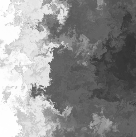
FIG. 17.: A snapshot of the scalar field, $T$, for the injection by a mean gradient directed from right to left. Colors are coded according to the intensity of the field: white corresponds to large positive values, black to large negative values.

The second scenario is based on the idea that the process of front formation starts from a $O(T_{rms})$ fluctuation of the scalar field generated at large scales by injection mechanisms. This profile gets steepened by the action of large-scale converging components of the velocity field, until the stretching exerted by small-scale velocity fluctuations overcomes the tendency of the front to steepen. As a result, the front survives only down to a scale $r$, larger than the dissipative scale $\eta$. The probability that the steepening process stops at a scale $r$ decreases with $r$ according to $r^{\zeta_{\infty}}$. At variance with the former picture, here the probability of observing a mature front vanishes as $\eta^{\zeta_{\infty}}$, thus it is strictly zero for an infinite Péclet number.

It has to be remarked that in both cases, the dimension of the set hosting mature fronts has to be $D_{F}=2-\zeta_{\infty}$, but the number of points which belong to this set is vanishing with increasing Péclet. Thus, the observation of a dimension $D_{F}\simeq 0.6$ (see Fig. 19 ) does not allow us to discriminate between the first and the second picture.

FIG. 18.: The union of the sets where mature fronts are located. The snapshots over which the union is performed are $80$, regularly spaced by one eddy turnover time.

FIG. 19.: The box-covering dimension of the mature cliffs set. The number of boxes of size $r$ necessary to cover the set represented in Fig. 18 decays as $N(r)\sim r^{-D_{F}}$ with $D_{F}=0.6$.

In a nutshell, in the first scenario intense small-scale excursion of scalar field are essentially generated by mature fronts, whereas in the second one mature fronts play a statistically insignificant role.

In order to quantify the weight of mature fronts in the build-up of strong fluctuations and thus distinguish among the two options listed above, we computed the following conditional probability. Given a jump of height $|\delta_{r1}T|=O(T_{rms})$ across an interval $I_{1}$ of length $r_{1}$, we measure the largest excursion $\Delta_{r_{2}}=\max_{I_{2}}{|\delta_{r_{2}}T|}$ occurring on a sub-interval $I_{2}\subset I_{1}$ of length $r_{2}$. If the mature fronts dominate the statistics, as in the first scenario, a one-dimensional section of the scalar field then would look like a sequence of steps. The distribution of $\Delta_{r_{2}}$ should then be sharply peaked around $\delta_{r_{1}}T$ for any $r_{2}$. On the contrary, if mature fronts have a relatively little probability with respect to non-mature ones, the typical value for $\Delta_{r_{2}}$ moves to smaller and smaller values while decreasing $r_{2}$. In Figure 20 we show that the second possibility is realized, and thus non-mature fronts dominate the statistics of the large excursions.

FIG. 20.: The pdf of $\Delta_{r_{2}}$ – maximal excursion across a length $r_{2}$ – under the condition that an excursion larger than $2.5T_{rms}$ takes place at a scale $r_{1}$, for three different $r_{2}/r_{1}$. All distances belong to the inertial range.

Summarizing, saturation comes from a self-similar process and the signature of the exponent $\zeta_{\infty}$ is felt throughout the inertial range down to the dissipative scales. In this sense, both mature and non-mature structures carry the imprinting of saturation: indeed the dimensions of the set of mature and of the set of non-mature fronts are equal to $2-\zeta_{\infty}$. Nevertheless, since the appearance of a mature front is a relatively rare event, the dominant contribution to structure functions is due to non-mature cliffs.

VII Plateaux

Fronts separate regions of space where a very efficient mixing takes place, and fluctuations of the scalar field are small. To investigate the statistical signature of these plateaux we computed the low-order moments of scalar increments, shown in Fig. 21. We observe that the scaling exponents of negative order display an almost linear dependence on the order, close to $p/2$. Thus, the scalar field within the plateaux is not smooth but it is characterized by a Hölder exponent 1/2. This would entail a single rescaling factor, $r^{1/2}$, for the inner core of the pdf of scalar increments, which seems to be the case, as in Fig. 22. This result suggests that the nature of scalar turbulence within the plateaux could be understood in simple terms, although, to our knowledge, no definite explanation of these observations is available up to now.

FIG. 21.: Scaling exponents of structure functions for low, fractional orders, in the random-forced case. Moments are taken with absolute values. The dotted line is $p/2$.

FIG. 22.: Probability density functions of scalar increments for three separations within the inertial range, rescaled by $r^{1/2}$.

VIII Scalar Dissipation

Let us focus our attention on the passive scalar equation (1), in the presence of a random forcing (2). Denoting $\delta_{r}T\equiv T(\mathchoice{{\hbox{\boldmath$\displaystyle x$}}}{{\hbox{\boldmath$\textstyle x$}}}{{\hbox{\boldmath$\scriptstyle x$}}}{{\hbox{\boldmath$\scriptscriptstyle x$}}})-T(\mathchoice{{\hbox{\boldmath$\displaystyle x$}}}{{\hbox{\boldmath$\textstyle x$}}}{{\hbox{\boldmath$\scriptstyle x$}}}{{\hbox{\boldmath$\scriptscriptstyle x$}}}^{\prime})$ the scalar increment over the separation $\mathchoice{{\hbox{\boldmath$\displaystyle r$}}}{{\hbox{\boldmath$\textstyle r$}}}{{\hbox{\boldmath$\scriptstyle r$}}}{{\hbox{\boldmath$\scriptscriptstyle r$}}}=\mathchoice{{\hbox{\boldmath$\displaystyle x$}}}{{\hbox{\boldmath$\textstyle x$}}}{{\hbox{\boldmath$\scriptstyle x$}}}{{\hbox{\boldmath$\scriptscriptstyle x$}}}-\mathchoice{{\hbox{\boldmath$\displaystyle x$}}}{{\hbox{\boldmath$\textstyle x$}}}{{\hbox{\boldmath$\scriptstyle x$}}}{{\hbox{\boldmath$\scriptscriptstyle x$}}}^{\prime}$, it is easy to obtain [19] the equation for the even-integer structure functions $S_{2n}$ (odd-integer structure functions are trivially vanishing for isotropic injection mechanisms):

$$\frac{\partial S_{2n}(r)}{\partial t}+\mathchoice{{\hbox{\boldmath$\displaystyle\nabla$}}}{{\hbox{\boldmath$\textstyle\nabla$}}}{{\hbox{\boldmath$\scriptstyle\nabla$}}}{{\hbox{\boldmath$\scriptscriptstyle\nabla$}}}\cdot\langle\mathchoice{{\hbox{\boldmath$\displaystyle W$}}}{{\hbox{\boldmath$\textstyle W$}}}{{\hbox{\boldmath$\scriptstyle W$}}}{{\hbox{\boldmath$\scriptscriptstyle W$}}}(\delta_{r}T)^{2n}\rangle=J_{2n}(r)$$ (21)

where

$$J_{2n}\equiv 2n\langle(\delta_{r}T)^{2n-1}H\rangle,$$ (22)

and

$$\mathchoice{{\hbox{\boldmath$\displaystyle W$}}}{{\hbox{\boldmath$\textstyle W$}}}{{\hbox{\boldmath$\scriptstyle W$}}}{{\hbox{\boldmath$\scriptscriptstyle W$}}}\equiv\langle\left[\mathchoice{{\hbox{\boldmath$\displaystyle v$}}}{{\hbox{\boldmath$\textstyle v$}}}{{\hbox{\boldmath$\scriptstyle v$}}}{{\hbox{\boldmath$\scriptscriptstyle v$}}}(\mathchoice{{\hbox{\boldmath$\displaystyle x$}}}{{\hbox{\boldmath$\textstyle x$}}}{{\hbox{\boldmath$\scriptstyle x$}}}{{\hbox{\boldmath$\scriptscriptstyle x$}}},t)-\mathchoice{{\hbox{\boldmath$\displaystyle v$}}}{{\hbox{\boldmath$\textstyle v$}}}{{\hbox{\boldmath$\scriptstyle v$}}}{{\hbox{\boldmath$\scriptscriptstyle v$}}}(\mathchoice{{\hbox{\boldmath$\displaystyle x$}}}{{\hbox{\boldmath$\textstyle x$}}}{{\hbox{\boldmath$\scriptstyle x$}}}{{\hbox{\boldmath$\scriptscriptstyle x$}}}^{\prime},t)\right]|\delta_{r}T\rangle,$$ (23)

$$H\equiv\langle\kappa\left(\Delta+\Delta^{\prime}\right)\delta_{r}T|\delta_{r}T\rangle$$ (24)

are the ensemble average of velocity increment and dissipation conditioned on the scalar increment $\delta_{r}T$, respectively. The Laplace operators in (24) are evaluated at $\textstyle x$ and $\mathchoice{{\hbox{\boldmath$\displaystyle x$}}}{{\hbox{\boldmath$\textstyle x$}}}{{\hbox{\boldmath$\scriptstyle x$}}}{{\hbox{\boldmath$\scriptscriptstyle x$}}}^{\prime}$ respectively. In our DNS simulations we replaced the Laplace operator in Eq. (1) with a bi-Laplacian dissipative term. The definition of the conditional dissipation $H$ is thus : $H(\delta_{r}T)\equiv-\kappa\langle\left(\Delta^{2}+(\Delta^{\prime})^{2}\right)\delta_{r}T|\delta_{r}T\rangle$. The choice of a laplacian or a bilaplacian is immaterial to all the forthcoming arguments. In isotropic conditions the vector $\textstyle W$ has the form $\mathchoice{{\hbox{\boldmath$\displaystyle W$}}}{{\hbox{\boldmath$\textstyle W$}}}{{\hbox{\boldmath$\scriptstyle W$}}}{{\hbox{\boldmath$\scriptscriptstyle W$}}}=W\hat{\mathchoice{{\hbox{\boldmath$\displaystyle r$}}}{{\hbox{\boldmath$\textstyle r$}}}{{\hbox{\boldmath$\scriptstyle r$}}}{{\hbox{\boldmath$\scriptscriptstyle r$}}}}$, and is even under a sign reversal of the scalar field, whereas $H$ is odd. The information carried by the set of equations (21), which hold for any $n$, can be expressed in a single equivalent equation for the pdf of scalar differences

$$\partial_{t}{\cal P}(\delta_{r}T)+\mathchoice{{\hbox{\boldmath$\displaystyle\nabla$}}}{{\hbox{\boldmath$\textstyle\nabla$}}}{{\hbox{\boldmath$\scriptstyle\nabla$}}}{{\hbox{\boldmath$\scriptscriptstyle\nabla$}}}\cdot\left(\mathchoice{{\hbox{\boldmath$\displaystyle W$}}}{{\hbox{\boldmath$\textstyle W$}}}{{\hbox{\boldmath$\scriptstyle W$}}}{{\hbox{\boldmath$\scriptscriptstyle W$}}}{\cal P}(\delta_{r}T)\right)=-{\partial\over\partial\delta_{r}T}\left(H{\cal P}(\delta_{r}T)\right)\;.$$ (25)

In the statistically stationary state this equation provides a dynamic link among the three quantities $W,H,{\cal P}$. Let us give a few examples which will be relevant to our subject: $(i)$, if ${\cal P}$ is exponential and $H$ is linear, then $W$ is linear; $(ii)$, if ${\cal P}$ is exponential and $H$ is constant, then then $W$ is constant; $(iii)$, if ${\cal P}$ is Gaussian and $W$ is constant, then $H$ is inversely proportional to the scalar fluctuation.

FIG. 23.: The longitudinal component of the W function vs $\delta_{r}T$ for two different values of $r$ in the inertial range.

Let us now look in detail at the numerical results: $W$ is shown in Fig. 23. The negative part for large values of $\delta_{r}T$ is physically intuitive : the formation of strong cliffs amounts to the build-up of intense scalar gradients, and takes place whenever the gradient alignes with the eigenvector of the strain with a negative eigenvalue. In other words, to obtain a large fluctuation it is necessary that the flow favors the approaches of elements of fluid that were initially far apart and characterized by very different values of the scalar field. Conversely, the positive peak for small scalar fluctuations shows that the “plateaux” are regions of extremely efficient mixing, dominated by small-scale disordered velocity fluctuations with high turbulent diffusivity.
The conditional dissipation function $H({\delta_{r}T})$ is shown in Fig. 24. The curve closely follows the linear ansatz [19] up to values comparable to $T_{rms}$. For larger values the curve is however distorted and has a definite tendency to flatten out.

FIG. 24.: The conditional dissipation $H$ vs $\delta_{r}T$ for two different separations $r$ in the inertial range.

As discussed in Sec. V, the tails of scalar increment pdf’s ${\cal P}(\delta_{r}T)$ for various separations $r$ in the inertial range all collapse onto a single curve : ${\cal P}(\delta_{r}T)=r^{\zeta_{\infty}}Q({\delta_{r}T\over T_{rms}})$. The curve $r^{-\zeta_{\infty}}{\cal P}(\delta_{r}T)$ is shown in Fig. 25 for one separation in the inertial range. Its tails (and those of $Q$) decay roughly as an exponential.

FIG. 25.: The scalar increment pdf for a separation within the inertial range.

The one-point pdf was shown in Fig. 5 and clearly decays as a Gaussian in the random-forced case. As a consequence, the exponential tails observed in Fig. 25 cannot continue for ever and a sharper than Gaussian fall off (see the arguments of Sec. VIII) is expected to set in.

From the comparison of the graphs of $W$,$H$ and ${\cal P}$ it appears that for fluctuations small compared to $T_{rms}$ we are under the conditions $(i)$, with an almost linear $H$, an approximately exponential behavior for ${\cal P}$ and a $W\sim|\delta_{r}T|$. This regime is characteristic of “plateaux” where efficient mixing occurs ($W>0$) and dissipation is proportional to the intensity of the fluctuation. For larger values $\delta_{r}T$ of the order of a few $T_{rms}$ we can recognize the case $(ii)$, characterized by the presence of fronts. Here, the dissipation is not anymore proportional to the scalar excursion, rather tending to be independent of it. It has to be remarked that, although large gradients may develop within a front, they have a negligible statistical weight, so that the main contribution to the dissipation comes from relatively small fluctuations of the order $\kappa^{1/4}\epsilon_{\theta}^{1/2}\epsilon_{v}^{-1/4}$. The regime $(iii)$, where the strength of fluctuations is dominated by the one-point pdf, is out of reach for our statistics: indeed, a rough estimate of the amplitudes where this regime sets in is $10\,T_{rms}$.

When the velocity field is rapidly changing in time, the expression for $W$ can be derived analytically, a fact which allows for further considerations which are presented in Appendix B.

IX Scalar fluxes

The classical theory of scalar turbulence presented in Section II is based on the picture of a cascade of scalar fluctuations from large to small scales which takes place at a scale-independent rate $\epsilon_{\theta}$. More quantitatively, the constancy of the scalar flux is expressed by means of an exact relation, the Yaglom’s law, which in two dimensions reads

$$\langle\left[\delta_{r}\mathchoice{{\hbox{\boldmath$\displaystyle v$}}}{{\hbox{\boldmath$\textstyle v$}}}{{\hbox{\boldmath$\scriptstyle v$}}}{{\hbox{\boldmath$\scriptscriptstyle v$}}}\cdot\hat{\mathchoice{{\hbox{\boldmath$\displaystyle r$}}}{{\hbox{\boldmath$\textstyle r$}}}{{\hbox{\boldmath$\scriptstyle r$}}}{{\hbox{\boldmath$\scriptscriptstyle r$}}}}\right](\delta_{r}T)^{2}\rangle=-2\epsilon_{\theta}r\;.$$ (26)

for any $r$ within the inertial range of scales. In the anisotropic case this relation still holds for the projections onto the isotropic sector. In Fig. 26 we show the velocity-scalar-scalar correlation which appears in (26) computed numerically for both the mean gradient and the random forced case.

FIG. 26.: The Yaglom’s law for the shear-driven ($\times$) and the random-forced ($+$) case.

The statistics of the scalar flux displays as well a remarkable intermittency. To quantify it, let us introduce the fluctuating scalar flux through the scale $r$ as $\Pi_{r}=\delta_{r}v(\delta_{r}T)^{2}$. We consider moments $\langle|\Pi_{r}|^{p}\rangle\sim r^{\alpha_{p}}$, which have been studied in the context of experimental turbulence in Ref. [53]. As shown in Figure 27, the computed scaling exponents $\alpha_{p}$ deviate significantly from the dimensional prediction $\alpha_{p}=p$. The behavior of the exponents for large orders can be explained with the aid of the results of Section VIII. We observed that the average velocity fluctuation becomes nearly constant for large enough scalar fluctuations (see Fig. 23). In other words, at small scales we observe a weak correlation between the scalar and the velocity fluctuations. A very rough estimate, based on the assumption that velocity-scalar correlations are small, gives us $\alpha_{p}\sim p/3+\zeta_{2p}$ for large $p$, which is remarkably close to the observed values. This approximation suggests that there will be no saturation for $\alpha_{p}$, and that asymptotically $\alpha_{p}\simeq p/3+\zeta_{\infty}$. The experimental data reported in Ref.[53] support this picture.

FIG. 27.: Scaling exponents $\alpha_{p}$ for various moments of the scalar flux. The dotted line is the dimensional prediction $\alpha_{p}=p$ and the solid line is the asymptote $\alpha_{p}=p/3+\zeta_{\infty}$.

X Conclusions and perspectives

There are several turbulent systems other than passive scalars which are characterized by the presence of structures : “plumes” in turbulent convection, “vortex sheets” in shear-driven hydrodynamic turbulence and “current sheets” in magnetohydrodynamics. It is thus natural to ask whether some or all of the results obtained for passive scalars apply to these other systems.
Small-scale anisotropy. A phenomenology similar to the one for the passive scalar has been identified for Navier–Stokes turbulence in the presence of a homogeneous shear flow [54] and for kinematic magnetohydrodynamics both in the presence of incompressible [55] and compressible [56] velocity fields. Concerning Navier–Stokes turbulence, an anisotropic component of the vorticity third-order correlation is found to be independent of the Reynolds number in the presence of a large-scale shear [54]. A mecahnism in terms of coherent structures has also been proposed for the emergence of small scale anisotropy [54]. Even if the effect is less pronounced than in the passive scalar case, it is likely that large-scale anisotropies do not decay down to the small scales. The same happens in magnetohydrodynamics turbulence where it has been found that for incompressible velocity fields the hyperskewness of the magnetic field diverges at small scales [55]. No systematic study has been performed in the context of turbulent convection.
Universality. There is good agreement about the universality, with respect to energy pumping details, of scaling exponents in homogeneous and isotropic hydrodynamic turbulence. For anisotropic turbulence it appears that the exponents in the isotropic sector coincide with those found in isotropic turbulence [32]. A similar conclusion has been found analytically for simple models of kinematic magnetohydrodynamics [55, 56]. No results are up to now available for the full magnetohydrodynamics. As for turbulent convection, there the system is self sustained and does not need external forcing, thus the problem has to be rephrased in terms of universality with respect to boundary conditions. We are not aware of any extensive analysis of this issue.
Saturation. The intrinsic instability of vortex sheets seems to rule out the possibility of a saturation of intermittency for Navier-Stokes turbulence. Conversely, the extreme stability and strength of plumes in convective turbulence suggests that saturation may occur there. Indeed, buoyancy forces may collaborate with compressional contributions of large scale velocity leading to sharper and more long-lived fronts than those observed in passive scalar turbulence. The situation with the magnetohydrodynamics turbulence remains to be clarified.

Acknowledgements. Helpful discussions with M. Chertkov, A. Fairhall, U. Frisch, B. Galanti, R.H. Kraichnan, V. Lebedev, A. Noullez, J.-F. Pinton, I. Procaccia, A. Pumir and V. Yakhot are gratefully acknowledged. We benefited from the hospitality of the 1999 ESF-TAO Study Center. The INFM PRA Turbo (AC), the INFM PA GEPAIGG01 (AM) and the ERB-FMBI-CT96-0974 (AL) contracts are acknowledged. This work was supported in part by the European Commission under contract HPRN-CT-2000-00162 (“Nonideal Turbulence”). A.C. was supported by a “H. Poincaré” CNRS postdoctoral fellowship. Simulations were performed at IDRIS (no 991226) and at CINECA (INFM Parallel Computing Initiative).

A Dominant and subdominant terms in the structure functions

In order to have a better insight on the angular dependence of scalar structure functions, it is useful to consider a simple example where the problem can be tackled analytically. This is the case for the second order structure function in the Kraichnan advection model [24, 19]. In this model the velocity field $\mathchoice{{\hbox{\boldmath$\displaystyle v$}}}{{\hbox{\boldmath$\textstyle v$}}}{{\hbox{\boldmath$\scriptstyle v$}}}{{\hbox{\boldmath$\scriptscriptstyle v$}}}=\{v_{\alpha},\alpha=1,\ldots,d\}$ advecting the scalar is incompressible, isotropic, Gaussian, white-noise in time; it has homogeneous increments with power-law spatial correlations and a scaling exponent $\xi$ in the range $0<\xi<2$ :

$$\left\langle[v_{\alpha}(\mathchoice{{\hbox{\boldmath$\displaystyle r$}}}{{\hbox{\boldmath$\textstyle r$}}}{{\hbox{\boldmath$\scriptstyle r$}}}{{\hbox{\boldmath$\scriptscriptstyle r$}}},t)-v_{\alpha}(\mathchoice{{\hbox{\boldmath$\displaystyle 0$}}}{{\hbox{\boldmath$\textstyle 0$}}}{{\hbox{\boldmath$\scriptstyle 0$}}}{{\hbox{\boldmath$\scriptscriptstyle 0$}}},0)][v_{\beta}(\mathchoice{{\hbox{\boldmath$\displaystyle r$}}}{{\hbox{\boldmath$\textstyle r$}}}{{\hbox{\boldmath$\scriptstyle r$}}}{{\hbox{\boldmath$\scriptscriptstyle r$}}},t)-v_{\beta}(\mathchoice{{\hbox{\boldmath$\displaystyle 0$}}}{{\hbox{\boldmath$\textstyle 0$}}}{{\hbox{\boldmath$\scriptstyle 0$}}}{{\hbox{\boldmath$\scriptscriptstyle 0$}}},0)]\right\rangle=$$ (A1)

$$\qquad 2\delta(t)D_{\alpha\beta}(\mathchoice{{\hbox{\boldmath$\displaystyle r$}}}{{\hbox{\boldmath$\textstyle r$}}}{{\hbox{\boldmath$\scriptstyle r$}}}{{\hbox{\boldmath$\scriptscriptstyle r$}}}),$$ (A2)

where,

$$D_{\alpha\beta}(\mathchoice{{\hbox{\boldmath$\displaystyle r$}}}{{\hbox{\boldmath$\textstyle r$}}}{{\hbox{\boldmath$\scriptstyle r$}}}{{\hbox{\boldmath$\scriptscriptstyle r$}}})=D_{0}r^{\xi}\left[\left(\xi+d-1\right)\delta_{\alpha\beta}-\xi\,{r_{\alpha}r_{\beta}\over r^{2}}\right].$$ (A3)

The specific form inside the squared brackets follows from the incompressibility condition on $\textstyle v$.

As remarked in Sec. V B, because of the white-in-time velocity field, this model leads to closed equations for single-time multiple-space correlation functions such as $C_{n}\equiv\left\langle\theta(\mathchoice{{\hbox{\boldmath$\displaystyle r$}}}{{\hbox{\boldmath$\textstyle r$}}}{{\hbox{\boldmath$\scriptstyle r$}}}{{\hbox{\boldmath$\scriptscriptstyle r$}}}_{1},t)\ldots\theta(\mathchoice{{\hbox{\boldmath$\displaystyle r$}}}{{\hbox{\boldmath$\textstyle r$}}}{{\hbox{\boldmath$\scriptstyle r$}}}{{\hbox{\boldmath$\scriptscriptstyle r$}}}_{n},t)\right\rangle$ at any order $n$ (see, e.g., Refs. [24, 41]).

Their general form in the stationary state (i.e. $\partial_{t}C_{n}=0$) maintained by the large scale gradient $\textstyle g$ is [41]:

$$\sum^{n}_{i\neq j}\left[D_{\alpha\beta}(\mathchoice{{\hbox{\boldmath$\displaystyle r$}}}{{\hbox{\boldmath$\textstyle r$}}}{{\hbox{\boldmath$\scriptstyle r$}}}{{\hbox{\boldmath$\scriptscriptstyle r$}}}_{i}-\mathchoice{{\hbox{\boldmath$\displaystyle r$}}}{{\hbox{\boldmath$\textstyle r$}}}{{\hbox{\boldmath$\scriptstyle r$}}}{{\hbox{\boldmath$\scriptscriptstyle r$}}}_{j})+\kappa\delta_{\alpha\beta}\right]\partial^{\alpha}_{r_{i}}\partial^{\beta}_{r_{j}}\langle\theta(\mathchoice{{\hbox{\boldmath$\displaystyle r$}}}{{\hbox{\boldmath$\textstyle r$}}}{{\hbox{\boldmath$\scriptstyle r$}}}{{\hbox{\boldmath$\scriptscriptstyle r$}}}_{1})\ldots\theta(\mathchoice{{\hbox{\boldmath$\displaystyle r$}}}{{\hbox{\boldmath$\textstyle r$}}}{{\hbox{\boldmath$\scriptstyle r$}}}{{\hbox{\boldmath$\scriptscriptstyle r$}}}_{n})\rangle$$ (A4)

$$= \sum^{n}_{i\neq j}g_{\alpha}g_{\beta}G_{\alpha\beta}(\mathchoice{{\hbox{\boldmath$\displaystyle r$}}}{{\hbox{\boldmath$\textstyle r$}}}{{\hbox{\boldmath$\scriptstyle r$}}}{{\hbox{\boldmath$\scriptscriptstyle r$}}}_{i}-\mathchoice{{\hbox{\boldmath$\displaystyle r$}}}{{\hbox{\boldmath$\textstyle r$}}}{{\hbox{\boldmath$\scriptstyle r$}}}{{\hbox{\boldmath$\scriptscriptstyle r$}}}_{j})\langle\theta(\mathchoice{{\hbox{\boldmath$\displaystyle r$}}}{{\hbox{\boldmath$\textstyle r$}}}{{\hbox{\boldmath$\scriptstyle r$}}}{{\hbox{\boldmath$\scriptscriptstyle r$}}}_{1})\smash{\mathop{\dots\dots}_{\hat{i}\ \ \hat{j}}}\theta(\mathchoice{{\hbox{\boldmath$\displaystyle r$}}}{{\hbox{\boldmath$\textstyle r$}}}{{\hbox{\boldmath$\scriptstyle r$}}}{{\hbox{\boldmath$\scriptscriptstyle r$}}}_{n})\rangle$$ (A5)

$$- 2\sum^{n}_{i\neq j}g_{\alpha}D_{\alpha\beta}(\mathchoice{{\hbox{\boldmath$\displaystyle r$}}}{{\hbox{\boldmath$\textstyle r$}}}{{\hbox{\boldmath$\scriptstyle r$}}}{{\hbox{\boldmath$\scriptscriptstyle r$}}}_{i}-\mathchoice{{\hbox{\boldmath$\displaystyle r$}}}{{\hbox{\boldmath$\textstyle r$}}}{{\hbox{\boldmath$\scriptstyle r$}}}{{\hbox{\boldmath$\scriptscriptstyle r$}}}_{j})\partial^{b}_{r_{j}}\langle\theta(\mathchoice{{\hbox{\boldmath$\displaystyle r$}}}{{\hbox{\boldmath$\textstyle r$}}}{{\hbox{\boldmath$\scriptstyle r$}}}{{\hbox{\boldmath$\scriptscriptstyle r$}}}_{1})\smash{\mathop{\dots\dots}_{\hat{i}}}\theta(\mathchoice{{\hbox{\boldmath$\displaystyle r$}}}{{\hbox{\boldmath$\textstyle r$}}}{{\hbox{\boldmath$\scriptstyle r$}}}{{\hbox{\boldmath$\scriptscriptstyle r$}}}_{n})\rangle,$$ (A6)

with $G_{\alpha\beta}(\mathchoice{{\hbox{\boldmath$\displaystyle r$}}}{{\hbox{\boldmath$\textstyle r$}}}{{\hbox{\boldmath$\scriptstyle r$}}}{{\hbox{\boldmath$\scriptscriptstyle r$}}})=\langle v_{\alpha}(\mathchoice{{\hbox{\boldmath$\displaystyle r$}}}{{\hbox{\boldmath$\textstyle r$}}}{{\hbox{\boldmath$\scriptstyle r$}}}{{\hbox{\boldmath$\scriptscriptstyle r$}}},t)v_{\beta}(\mathchoice{{\hbox{\boldmath$\displaystyle 0$}}}{{\hbox{\boldmath$\textstyle 0$}}}{{\hbox{\boldmath$\scriptstyle 0$}}}{{\hbox{\boldmath$\scriptscriptstyle 0$}}},t)\rangle$ and where the translational invariance of scalar correlation functions has been exploited. For the sake of simplicity, let us focus the attention on the equation for the two-point correlation function $C_{2}(r,\phi)$ in the two-dimensional case, with $\phi$ denoting the angle between the mean gradient $\textstyle g$ and the separation $\textstyle r$. Restricting ourselves to the inertial range of scales, such equation has the simple form

$$- \left[\frac{1}{r}\partial_{r}(r^{\xi+1}\partial_{r})\,+\,\frac{\xi+1}{r^{2-\xi}}\partial^{2}_{\phi}\right]\,C_{2}(r,\phi)$$ (A7)

$$= g^{2}-g^{2}r^{\xi}\left[(\xi+1)-\xi\cos^{2}\phi\right].$$ (A8)

Among the possible functional basis through which $C_{2}(r,\phi)$ can be decomposed, the SO(2) representation functions [57] $U^{(l)}(\phi)\equiv\exp(-i\,l\phi)$ turns out to be particularly useful [58]. Indeed, exploiting this representation we have

$$C_{2}(r,\phi)=\sum_{l=0}C^{(2l)}_{2}(r)\cos[(2l)\phi],$$ (A9)

(only even values of $l$ are involved due to the invariance of $C_{2}(r,\phi)$ under the transformation $\phi\mapsto\phi+\pi$) and the equations for each of the projections $C^{(2l)}_{2}(r)$ are closed and independent, and can thus be separately solved. It is easy to show that the solution for the isotropic component $C^{(0)}_{2}(r)$ is simply :

$$C^{(0)}_{2}(r)=const-\frac{g^{2}L^{\xi}}{2(2-\xi)}r^{2-\xi}+\frac{g^{2}}{4}r^{2},$$ (A10)

where the dimensional constant appearing in the right hand side is the only non-trivial homogeneous solution (zero mode), of the equation for the second order correlation function. Here, $L$ is the integral scale of the problem. It then follows that the structure function in the isotropic sector $l=0$ is proportional to $\frac{g^{2}L^{\xi}}{2(2-\xi)}r^{2-\xi}-\frac{g^{2}}{4}r^{2}$, i.e. a sum of power laws. Conversely, the structure function $\langle\left(T(\mathchoice{{\hbox{\boldmath$\displaystyle r$}}}{{\hbox{\boldmath$\textstyle r$}}}{{\hbox{\boldmath$\scriptstyle r$}}}{{\hbox{\boldmath$\scriptscriptstyle r$}}})-T(\mathchoice{{\hbox{\boldmath$\displaystyle 0$}}}{{\hbox{\boldmath$\textstyle 0$}}}{{\hbox{\boldmath$\scriptstyle 0$}}}{{\hbox{\boldmath$\scriptscriptstyle 0$}}})\right)^{2}\rangle$ for the total field $T(\mathchoice{{\hbox{\boldmath$\displaystyle r$}}}{{\hbox{\boldmath$\textstyle r$}}}{{\hbox{\boldmath$\scriptstyle r$}}}{{\hbox{\boldmath$\scriptscriptstyle r$}}})=\theta(\mathchoice{{\hbox{\boldmath$\displaystyle r$}}}{{\hbox{\boldmath$\textstyle r$}}}{{\hbox{\boldmath$\scriptstyle r$}}}{{\hbox{\boldmath$\scriptscriptstyle r$}}})+\mathchoice{{\hbox{\boldmath$\displaystyle g$}}}{{\hbox{\boldmath$\textstyle g$}}}{{\hbox{\boldmath$\scriptstyle g$}}}{{\hbox{\boldmath$\scriptscriptstyle g$}}}\cdot\mathchoice{{\hbox{\boldmath$\displaystyle r$}}}{{\hbox{\boldmath$\textstyle r$}}}{{\hbox{\boldmath$\scriptstyle r$}}}{{\hbox{\boldmath$\scriptscriptstyle r$}}}$ in the isotropic sector goes as :

$$S_{2}^{(0)}(r)=\frac{g^{2}L^{\xi}}{2(2-\xi)}r^{2-\xi}.$$ (A11)

This means that the two structure functions, for the fluctuating field $\theta(\mathchoice{{\hbox{\boldmath$\displaystyle r$}}}{{\hbox{\boldmath$\textstyle r$}}}{{\hbox{\boldmath$\scriptstyle r$}}}{{\hbox{\boldmath$\scriptscriptstyle r$}}})$ and for the total field $T(\mathchoice{{\hbox{\boldmath$\displaystyle r$}}}{{\hbox{\boldmath$\textstyle r$}}}{{\hbox{\boldmath$\scriptstyle r$}}}{{\hbox{\boldmath$\scriptscriptstyle r$}}})$ behave, in the isotropic sector, in the same way $\propto r^{2-\xi}$, with decreasing $r$; but while those for $\theta(\mathchoice{{\hbox{\boldmath$\displaystyle r$}}}{{\hbox{\boldmath$\textstyle r$}}}{{\hbox{\boldmath$\scriptstyle r$}}}{{\hbox{\boldmath$\scriptscriptstyle r$}}})$ are sums of power laws, structure functions of $T(\mathchoice{{\hbox{\boldmath$\displaystyle r)$}}}{{\hbox{\boldmath$\textstyle r)$}}}{{\hbox{\boldmath$\scriptstyle r)$}}}{{\hbox{\boldmath$\scriptscriptstyle r)$}}}$ have a pure power law scaling. It is then useful to work with the total field $T(\mathchoice{{\hbox{\boldmath$\displaystyle r$}}}{{\hbox{\boldmath$\textstyle r$}}}{{\hbox{\boldmath$\scriptstyle r$}}}{{\hbox{\boldmath$\scriptscriptstyle r$}}})$ to obtain cleaner scaling behaviors.

B Scalar dissipation and saturation in the Kraichnan model

Let us now specialize the analysis (see also Ref. [59]) for the Kraichnan advection model (A2). Exploiting homogeneity, incompressibility and the $\delta$-correlation in time, $\mathchoice{{\hbox{\boldmath$\displaystyle\nabla$}}}{{\hbox{\boldmath$\textstyle\nabla$}}}{{\hbox{\boldmath$\scriptstyle\nabla$}}}{{\hbox{\boldmath$\scriptscriptstyle\nabla$}}}\cdot\langle\mathchoice{{\hbox{\boldmath$\displaystyle W$}}}{{\hbox{\boldmath$\textstyle W$}}}{{\hbox{\boldmath$\scriptstyle W$}}}{{\hbox{\boldmath$\scriptscriptstyle W$}}}(\delta_{r}T)^{2n}\rangle$ can be evaluated exactly and its expression reads [19]:

$$\mathchoice{{\hbox{\boldmath$\displaystyle\nabla$}}}{{\hbox{\boldmath$\textstyle\nabla$}}}{{\hbox{\boldmath$\scriptstyle\nabla$}}}{{\hbox{\boldmath$\scriptscriptstyle\nabla$}}}\cdot\langle\mathchoice{{\hbox{\boldmath$\displaystyle W$}}}{{\hbox{\boldmath$\textstyle W$}}}{{\hbox{\boldmath$\scriptstyle W$}}}{{\hbox{\boldmath$\scriptscriptstyle W$}}}(\delta_{r}T)^{2n}\rangle=-\frac{2}{r^{d-1}}\frac{\partial}{\partial r}\left(r^{d-1}\eta(r)\frac{\partial S_{2n}(r)}{\partial r}\right)$$ (B1)

where $\eta(r)=D_{0}(d-1)/2\,r^{\xi}$ is the relative diffusion operator. On the contrary, $J_{2n}(r)$ does not involves solely two-point averages and this means that, in general, it cannot be simply expressed in term of structure functions.
In the stationary state (i.e. $\partial S_{2n}/\partial t=0$) and for separations, $r$, in the inertial range of scales (i.e. $\eta_{\theta}\ll r\ll L$) a power-law behavior for $S_{2n}(r)$ (i.e. $S_{2n}(r)=s_{2n}r^{\zeta_{2n}}$) is expected. The same law, with exponent $\zeta_{2n}-\zeta_{2}$, holds for $J_{2n}$ to ensure the balance between the advective and the diffusive term, $J_{2n}$, in Eq. (21). Imposing the balance in Eq. (21) for power law coefficients and using (B1), the following equation is obtained:

$$\zeta_{2n}(d+\zeta_{2n}-\zeta_{2})=d\,\zeta_{2}\frac{j_{2n}}{s_{2n}}\frac{s_{2}}{j_{2}},$$ (B2)

where we have posed $J_{2n}=j_{2n}r^{\zeta_{2n}-\zeta_{2}}$.

Let us discuss the consequences of saturation on Eq. (21) and thus on (B2). When scaling exponents saturate, for $n\geq\overline{n}$ we have $\zeta_{2n}=\zeta_{\infty}$ and the left hand side of Eq. (B2) does not depend on $n$ any longer. To ensure the balance for all $n\geq\overline{n}$, the same independence on $n$ thus holds also in the right hand side of (B2), that implies:

$$\frac{j_{2n}}{s_{2n}}\frac{s_{2}}{j_{2}}=C\qquad\mbox{or}\qquad 2n\langle(\delta_{r}T)^{2n-1}H\rangle=CJ_{2}\frac{S_{2n}}{S_{2}}$$ (B3)

where $C$ may depends on $\xi$ and/or $d$, but not on $n$. Notice that complete saturation, i.e. $\zeta_{\infty}=\zeta_{2}$, yields $C=1$.
We now focus on the consequences of (B3) on the behavior vs $\delta_{r}T$ of $H(\delta_{r}T)$ and $K(\delta_{r}T)$, with

$$K\equiv\kappa\langle\left|\nabla\delta_{r}T+\nabla^{\prime}\delta_{r}T\right|^{2}|\delta_{r}T\rangle,$$ (B4)

a conditional mean related to dissipation.
To do that, we have to assume a specific form for the pdf of scalar increments ${\cal P}(\delta_{r}T)$. Our attention being focused on values of $\delta_{r}T\gtrsim T_{rms}$, so that ${\cal P}(\delta_{r}T)\propto r^{\zeta_{\infty}}{\cal Q}\left(\frac{\delta_{r}T}{T_{rms}}\right)$, statistical relations involving high-order structure functions (e.g. their ratio) are thus fully controlled by ${\cal Q}$. As a first choice, fully justified solely for the extreme tails $\delta_{r}T\gg T_{rms}$, we can thus assume a Gaussian shape for ${\cal Q}$. When doing this, recalling that for a Gaussian pdf we have $\langle(\delta_{r}T)^{2n}\rangle=(2n-1)\langle(\delta_{r}T)^{2n-2}\rangle$, we immediately realize that the second of (B3) is satisfied by

$$H=C\frac{J_{2}}{\delta_{r}T\,S_{2}}\qquad\mbox{for}\qquad\delta_{r}T\gg T_{rms}.$$ (B5)

It is now possible to show that, as a consequence of homogeneity alone (see Ref. [60]) $H$ and $K$ are related by the following identity:

$$H\,P\equiv\frac{\partial}{\partial\delta_{r}T}[K\,P],$$ (B6)

from which, using the Gaussianity of ${\cal Q}$, one obtains that at large values of $\delta_{r}T$ : $K\propto\frac{H}{\delta_{r}T}$.
It immediately follows according to (B5) that the conditional mean $K$ behaves as

$$K\propto\frac{H}{\delta_{r}T}\propto\frac{1}{(\delta_{r}T)^{2}}.$$ (B7)

We have already stressed that the behaviors vs $\delta_{r}T$ of the conditional means $H(\delta_{r}T)$ and $K(\delta_{r}T)$ depend on the specific assumption made on the asymptotic shape of ${\cal Q}$. However, in most experimental situations, one does not have access to the strongest events controlling the extreme tails of ${\cal Q}$. Although one can clearly observe the rescaling (16) and thus gather information on the saturation, ${\cal Q}$ might still not have relaxed on the single point pdf.
To better illustrate this point, let us assume that we can control scalar increments statistics for $\delta_{r}T\gtrsim T_{rms}$, but far from the asymptotic situation $\delta_{r}T\gg T_{rms}$. We thus rule out Gaussianity for ${\cal Q}$ and assume a slower decaying, e.g. of exponential type, as suggested by the numerical results. When doing this, recalling that for an exponential pdf we have $\langle(\delta_{r}T)^{2n}\rangle=2n\langle(|\delta_{r}T|)^{2n-1}\rangle$, we immediately realize that the second equation in (B3) is now satisfied by

$$H=sign(\delta_{r}T)\frac{C\,J_{2}}{S_{2}}\qquad\mbox{for}\qquad\delta_{r}T\gtrsim T_{rms}.$$ (B8)

From the identity (B6), it also follows that $K$ is now $\propto H$. We can conclude that, at least in the range $\delta_{r}T\gtrsim T_{rms}$ (but still far from $\delta_{r}T\gg T_{rms}$) and for an exponential decay of ${\cal Q}$ in (16), saturation is thus compatible with the behaviors of $H$ and $K$ displaying no dependence on $\delta_{r}T$.

REFERENCES

- [1] B.I. Shraiman and E.D. Siggia, “Scalar turbulence,” Nature 405, 639 (2000).
- [2] F. Dalaudier, C. Sidi, M. Crochet, and J. Vernin, “Direct evidences of “sheet” in the atmospheric temperature field,” J. Atmos. Sci. 51, 237 (1994).
- [3] E.E. Gossard, J.E. Gaynor, R.J. Zamora, and W.D. Neff, “Finestructure of elevated stable layers observed by sounder and in situ tower sensors,” J. Atmos. Sci. 42, 2156 (1985).
- [4] M.C. Gregg, “Microstructure patches in the thermocline,” J. Phys. Oceanogr. 10, 915 (1980).
- [5] R.G. Luek, “Turbulent mixing at the Pacific subtropical front,” J. Phys. Oceanogr. 18, 1761 (1988).
- [6] C.H. Gibson, C.A. Freihe, and S.O. McConnell, “Skewness of temperature derivatives in turbulent shear flows,” Phys. Fluids Supp. 20, S156, (1977).
- [7] P.G. Mestayer, “Local isotropy and anisotropy in a high-Reynolds-number turbulent boundary layer,” J. Fluid Mech. 125, 475, (1982).
- [8] K.R. Sreenivasan, “On local isotropy of passive scalars in turbulent shear flows,” Proc. Roy. Soc. London A434, 165, (1991).
- [9] L. Mydlarski and Z. Warhaft, “ Passive scalar statistics in high-Péclet-number grid turbulence,” J. Fluid Mech. 358, 135, (1998).
- [10] E.P. Salathé and R.B.. Smith, “In situ observations of temperature microstructure above and below the tropopause,” J. Atmos. Sci. 49, 2032 (1992).
- [11] J. Pedlosky, Geophysical fluid dynamics (Springer, New York, 1987).
- [12] P. Constantin, A. Majda, and E. Tabak, “Formation of strong fronts in the 2-D quasigeostrophic thermal active scalar,” Nonlinearity 7, 1495 (1994).
- [13] A. Pumir, “A numerical study of the mixing of a passive scalar in three dimensions in the presence of a mean gradient,” Phys. Fluids 6, 2118 (1994).
- [14] A. Celani, A. Lanotte, A. Mazzino, and M. Vergassola, “Universality and saturation of intermittency in passive scalar turbulence,” Phys. Rev. Lett. 84, 2385 (2000)
- [15] M. Holzer and E.D. Siggia, “Turbulent mixing of a passive scalar,” Phys. Fluids 6, 1820 (1994); Erratum, Phys. Fluids 7, 1519 (1995).
- [16] M. Vergassola and A. Mazzino, “Structures and intermittency in a passive scalar model,” Phys. Rev. Lett. 79, 1849 (1997).
- [17] A.L. Fairhall, B. Galanti, V.S. L’vov, and I. Procaccia, “Direct Numerical Simulations of the Kraichnan Model: Scaling Exponents and Fusion Rules,” Phys. Rev. Lett. 79, 4166 (1997).
- [18] S. Chen and R. H. Kraichnan, “Simulations of a randomly advected passive scalar field,” Phys. Fluids 68, 2867 (1998).
- [19] R.H. Kraichnan, “Anomalous scaling of a randomly advected passive scalar,” Phys. Rev. Lett. 72, 1016 (1994).
- [20] J. Weiss, “The dynamics of enstrophy transfer in two-dimensional hydrodynamics,” Physica D 48, 273 (1991).
- [21] H. Tennekes and J.L. Lumley, A first course in turbulence (MIT Press, Cambridge, MA, 1972).
- [22] J.L. Lumley, “Similarity and the Turbulent Energy Spectrum,” Phys. Fluids 10, 855 (1967).
- [23] R.H. Kraichnan, “Inertial ranges in two-dimensional turbulence,” Phys. Fluids 10, 1417 (1967).
- [24] R.H. Kraichnan, “Small-scale structure of a scalar field convected by turbulence,” Phys. Fluids 11, 945 (1968).
- [25] G. Boffetta, A. Celani, and M. Vergassola, “Inverse cascade in two-dimensional turbulence: deviations from Gaussianity,” Phys. Rev. E 61, R29 (2000).
- [26] U. Frisch, Turbulence, Cambridge Univ. Press, Cambridge, (1995).
- [27] L. Smith and V. Yakhot, “Bose condensation and small-scale structure generation in a random force driven 2D turbulence” Phys. Rev. Lett. 71, 352, (1993).
- [28] J. Paret and P. Tabeling, “Intermittency in the two-dimensional inverse cascade of energy: Experimental observations,” Phys. Fluids 10, 3126, (1998).
- [29] V. Yakhot, “Two-dimensional turbulence in the inverse cascade range,” Phys. Rev. E 60, 5544 (1999).
- [30] C. Tong and Z. Warhaft, “On passive scalar derivative statistics in grid turbulence,” Phys. Fluids 6, 2165 (1994).
- [31] I. Arad, B. Dhruva, S. Kurien, V.S. L’Vov, I. Procaccia, and K.R. Sreenivasan, “Extraction of anisotropic contributions in turbulent flows,” Phys. Rev. Lett. 81, 5330 (1998).
- [32] I. Arad, L. Biferale, I. Mazzitelli, and I. Procaccia, “Disentangling scaling properties in anisotropic and inhomogeneous turbulence,” Phys. Rev. Lett. 82, 5040 (1999).
- [33] A. Pumir, B. I. Shraiman, and E.D. Siggia, “Exponential tails and random advection,” Phys. Rev. Lett. 66, 2984 (1991).
- [34] M. Chertkov, G. Falkovich, I. Kolokolov, and V. Lebedev, “Statistics of a passive scalar advected by a large-scale 2D velocity field: analytic solution,” Phys. Rev. E 51, 5609, (1995).
- [35] Jayesh, and Z. Warhaft, “Probability distributions of a passive scalar in grid-generated turbulence,” Phys. Rev. Lett. 67, 3503 (1991).
- [36] K. Gawȩdzki and A. Kupiainen, “Anomalous scaling of the passive scalar,” Phys. Rev. Lett. 75, 3834 (1995).
- [37] M. Chertkov, G. Falkovich, I. Kolokolov, and V. Lebedev, “Normal and anomalous scaling of the fourth-order correlation function of a randomly advected passive scalar,” Phys. Rev. E 2, 4924 (1995).
- [38] B.I. Shraiman and E.D. Siggia, “Anomalous scaling of a passive scalar in turbulent flow,” C. R. Acad. Sci. Paris, série II 321, 279 (1995).
- [39] A. Noullez, G. Wallace, W. Lempert, R.B. Miles, and U. Frisch, J. Fluid Mech. 339, 287 (1997).
- [40] U. Frisch, A. Mazzino, A. Noullez, and M. Vergassola, “Lagrangian method for multiple correlations in passive scalar advection,” Phys. Fluids 11, 2178 (1999).
- [41] B.I. Shraiman and E.D. Siggia, “Lagrangian path integrals and fluctuations in random flow,” Phys. Rev. E 49, 2912 (1994).
- [42] M. Vergassola, “Anomalous scaling for passively advected magnetic fields,” Phys. Rev. E 53, R3021 (1996).
- [43] R. Benzi, L. Biferale, and A. Wirth, “Analytic Calculation of Anomalous Scaling in Random Shell Models for a Passive Scalar,” Phys. Rev. Lett. 78, 26 (1997).
- [44] A. Pumir, “Anomalous scaling behaviour of a passive scalar in the presence of a mean gradient,” Europhys. Lett. 34, 25 (1996).
- [45] L.Ts. Adzhemyan, N.V. Antonov, and A.N. Vasil’ev, “Renormalization group, operator product expansion, and anomalous scaling in a model of advected passive scalar,” Phys. Rev. E. 58, 1823 (1998).
- [46] L. N. Lipatov, JETP Lett.24 157 (1976), Sov. Phys. JETP 44 1055 (1976), JETP Lett.25 104 (1977), Sov. Phys. JETP 45 216 (1977).
- [47] J. Zinn-Justin, Quantum Field Theory and Critical Phenomena, Oxford University press, Oxford (1989).
- [48] E. Balkovsky and V. Lebedev, “Instanton for the Kraichnan passive scalar problem,” Phys. Rev. E 58, 5776 (1998).
- [49] V. Yakhot, “Passive scalar advected by a rapidly changing random velocity field: probability density of scalar differences,” Phys. Rev. E 55, 329 (1997).
- [50] M. Chertkov, “Instanton for random advection,” Phys. Rev. E 55, 2722 (1997).
- [51] U. Frisch, A. Mazzino, and M. Vergassola, “Intermittency in passive scalar advection,” Phys. Rev. Lett. 80, 5532 (1998).
- [52] E. Aurell, U. Frisch, J. Lutsko, and M. Vergassola, “On the multifractal properties of the energy dissipation derived from turbulence data”, J. Fluid Mech. 238, 467 (1992).
- [53] E. Lévêque, G. R. Ruiz-Chavarria, C. Baudet and S. Ciliberto, “Scaling laws for the turbulent mixing of a passive scalar in the wake of a cylinder”, Phys. Fluids 11, 1869 (1999).
- [54] A. Pumir and B.I. Shraiman, “Persistent small scale anisotropy in homogeneous shear flow,” Phys. Rev. Lett. 75, 3114 (1995).
- [55] N.V. Antonov, A. Lanotte, and A. Mazzino, “Persistence of small-scale anisotropies and anomalous scaling in a model of magnetohydrodynamics turbulence,” Phys. Rev. E 61, 6586 (2000)
- [56] N.V. Antonov, Y. Honkonen, A. Mazzino, and P. Muratore-Ginanneschi, “Manifestation of anisotropy persistence in the hierarchies of MHD scaling exponents,” (to appear in Phys. Rev. E), E-print archive nlin.CD/0005019.
- [57] W. Tung, Group theory in Physics, (World Scientific, Singapore, 1985).
- [58] I. Arad, V.S. L’Vov, E. Podivilov, and I. Procaccia, “Anomalous Scaling in the Anisotropic Sectors of the Kriachnan Model of Passive Scalar Advection,” E-print archive chao-dyn/9907017.
- [59] R.H. Kraichnan, “Passive scalar: scaling exponents and realizability,” Phys. Rev. Lett. 78, 4922 (1997).
- [60] S.B. Pope and E.S.C. Ching, “Stationary probability density functions in turbulence,” Phys. Fluids 5, 1529 (1993).