Abstract

This paper deals with feedback control of fractional-order Chua’s system. The fractional-order Chua’s system with total order less than three which exhibit chaos as well as other nonlinear behavior and theory for control of chaotic systems using sampled data are presented. Numerical experimental example is shown to verify the theoretical results.

1 Introduction

It is well known that chaos cannot occur in continuous systems of total order less than three. This assertion is based on the usual concepts of order, such as the number of states in a system or the total number of separate differentiations or integrations in the system. The model of system can be rearranged to three single differential equations, where one of the equations contains the non-integer (fractional) order derivative. The total order of system is changed from $3$ to $2+q$, where $0<q\leq 1$. To put this fact into context, we can consider the fractional-order dynamical model of the system. Hartley et al. [4] consider the fractional-order Chua’s system and demonstrated that chaos is possible for systems where the order is less than three. In their work, the limits on the mathematical order of the system to have a chaotic response, as measured from the bifurcation diagrams, are approximately from $2.5$ to $3.8$. In work [1], chaos was discovered in fractional-order two-cell cellular neural networks and also in work [6] chaos was exhibited in a system with total order less than three.

The control of chaos has been studied and observed in experiments (e.g. works [3], [5], [8], [12]). Especially, the control of well-known Chua’s system [9] by sampled data has been studied [13]. The main motivation for the control of chaos via sampled data is well-developed digital control techniques.

In this brief studies are presented practical results from sampled-data feed-back control of fractional-order chaotic dynamical system, modeled by the state equation $\dot{\bf x}={\bf f(x)}$, where ${\bf x}\in\Re^{n}$ is state variable, ${\bf f}:\Re^{n}\to\Re^{n}$ is nonlinear function and ${\bf f}(0)=0$.

The approach used in this paper is concentrating on the feed-back control of the chaotic fractional-order Chua’s system, where total order of the system is $2.9$.

2 Fractional calculus

2.1 Definitions of Fractional Derivatives

The idea of fractional calculus has been known since the development of the regular calculus, with the first reference probably being associated with Leibniz and L’Hospital in 1695.

Fractional calculus is a generalization of integration and differentiation to non-integer order fundamental operator ${}_{a}D^{\alpha}_{t}$, where $a$ and $t$ are the limits of the operation. The continuous integro-differential operator is defined as

$${}_{a}D^{\alpha}_{t}=\left\{\begin{array}[]{ll}\frac{d^{\alpha}}{dt^{\alpha}}&\mbox{$\Re(\alpha)>0$,}\\ 1&\mbox{$\Re(\alpha)=0$,}\\ \int_{a}^{t}(d\tau)^{-\alpha}&\mbox{$\Re(\alpha)<0$.}\end{array}\right.$$

The two definitions used for the general fractional differintegral are the Grünwald-Letnikov (GL) definition and the Riemann-Liouville (RL) definition [7], [11]. The GL is given here

$$_{a}D^{\alpha}_{t}f(t)=\lim_{h\to 0}h^{-\alpha}\sum_{j=0}^{[\frac{t-a}{h}]}(-1)^{j}{\alpha\choose j}f(t-jh),$$ (1)

where $[x]$ means the integer part of $x$. The RL definition is given as

$$_{a}D_{t}^{\alpha}f(t)=\frac{1}{\Gamma(n-\alpha)}\frac{d^{n}}{dt^{n}}\int_{a}^{t}\frac{f(\tau)}{(t-\tau)^{\alpha-n+1}}d\tau,\\$$ (2)

for $(n-1<\alpha<n)$ and where $\Gamma(.)$ is the Gamma function.

2.2 Numerical Methods for Calculation of Fractional
Derivatives

For numerical calculation of fractional-order derivation we can use the relation (3) derived from the Grünwald-Letnikov definition (1). This approach is based on the fact that a wide class of functions, two definitions - GL (1) and RL (2) - are equivalent. The relation for the explicit numerical approximation of $\alpha$-th derivative at the points $kT,\,(k=1,2,\dots)$ has the following form [2], [10], [11]:

$$_{(k-L/T)}D^{\alpha}_{kT}f(t)\approx T^{-\alpha}\sum_{j=0}^{k}(-1)^{j}{\alpha\choose j}f_{k-j},$$ (3)

where $L$ is the ”memory length”, $T$ is the step size of the calculation (sample period) and $(-1)^{j}{\alpha\choose j}$ are binomial coefficients $c_{j}^{(\alpha)},\,(j=0,1,\dots)$. For its calculation we can use the following expression:

$$c_{0}^{(\alpha)}=1,\qquad c_{j}^{(\alpha)}=\left(1-\frac{1+\alpha}{j}\right)c_{j-1}^{(\alpha)}.$$ (4)

2.3 Some Properties of Fractional Derivatives

Two general properties of fractional derivative we will be used. The first is composition of fractional with integer-order derivative and the second is the property of linearity.

The fractional-order derivative commutes with integer-order derivation [11],

$$\frac{d^{n}}{dt^{n}}(_{a}D^{p}_{t}f(t))=\,_{a}D^{p}_{t}\left(\frac{d^{n}f(t)}{dt^{n}}\right)=\,_{a}D_{t}^{p+n}f(t),$$ (5)

under the condition $t=a$ we have $f^{(k)}(a)=0,\,(k=0,1,2,\dots,n-1)$. The relationship (5) says the operators $\frac{d^{n}}{dt^{n}}$ and ${}_{a}D_{t}^{p}$ commute.

Similar to integer-order differentiation, fractional differentiation is a linear operation [11]:

$$_{a}D^{p}_{t}\left(\lambda f(t)+\mu g(t)\right)=\lambda\,_{a}D^{p}_{t}f(t)+\mu\,_{a}D^{p}_{t}g(t).$$ (6)

3 Fractional-Order Chua’s System

Classical Chua’s oscillator, which is shown in Fig. 1, is given by

$$\frac{dv_{1}}{dt} = \frac{1}{C_{1}}\left[G(v_{2}-v_{1})-f(v_{1})\right],$$

$$\frac{dv_{2}}{dt} = \frac{1}{C_{2}}\left[G(v_{1}-v_{2})+i\right],$$ (7)

$$\frac{di}{dt} = \frac{1}{L}\left[-v_{2}(t)-R_{L}i\right],$$

where $G=1/R$ and $f(v_{1})$ is the piecewise linear $v-i$ characteristic of nonlinear Chua’s diode.

Given the techniques of fractional calculus, there are still a number of ways in which the order of system could be amended. One approach would be to change the order of any or all of tree constitutive equations (3) so that the total order gave the desired value.

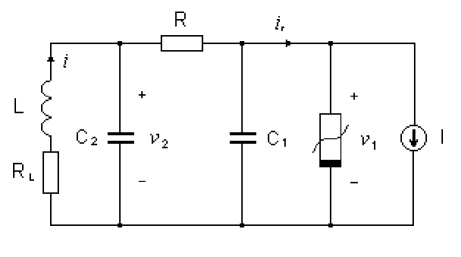
Figure 1: Chua’s circuit.

In our case, in the equation one, we replace the first differentiation by fractional differentiation of order $q$, $q\in\Re$. The final dimensionless equations of the system for $R_{L}=0$ are $(x_{1}=v_{1},x_{2}=v_{2},x_{3}=i)$:

$$\frac{dx_{1}(t)}{dt} = \alpha\,\,_{0}D^{1-q}_{t}\left(x_{2}(t)-x_{1}(t)-f(x_{1})\right),$$

$$\frac{dx_{2}(t)}{dt} = x_{1}(t)-x_{2}(t)+x_{3}(t),$$ (8)

$$\frac{dx_{3}(t)}{dt} = -\beta x_{2}(t),$$

where

$$f(x_{1})=bx_{1}+\frac{1}{2}(a-b)(|x_{1}+1|-|x_{1}-1|)$$

and $\alpha=C_{2}/C_{1}$, $\beta=C_{2}R^{2}/L$.

4 Feedback Control of Chaos

The structure of control system with sampled data [13] is shown in Fig. 2. The state variables of the chaotic system are measured and the result is used to construct the output signal ${\bf y}(t)=D{\bf x}(t)$, where $D$ is a constant matrix. The output ${\bf y}(t)$ is then sampled by sampling block to obtain ${\bf y}(k)=D{\bf x}(k)$ at the discrete moments $kT$, where $k=0,1,2,\dots$, and $T$ is the sample period. Then $D{\bf x}(k)$ is used by the controller to calculate the control signal ${\bf u}(k)$, which is fed back into chaotic system.

The controlled chaotic system is defined by relations [13]

$$\frac{d{\bf{x}(t)}}{dt} = {\bf{f}}({\bf x}(t))+B{\bf u}(k),\,\,\,\,\,t\in[kT,(k+1)T)$$

$${\bf u}(k+1) = C{\bf u}(k)+D{\bf x}(k),\,\,\,\,\,k=0,1,2,\dots$$ (9)

where ${\bf u}\in\Re^{m},\,B\in\Re^{n}\times\Re^{m},\,C\in\Re^{m}\times\Re^{m},\,D\in\Re^{m}\times\Re^{n}$ and $t\in R_{+}$; ${\bf x}(k)$ is the sampled value of ${\bf x}(t)$ at $t=kT$. Observe that since ${\bf f(0)=0}$ is an equilibrium point of the system (4).

The controlled fractional-order Chua’s system is defined by

$$\frac{dx_{1}(t)}{dt} = \alpha\,\,_{0}D^{1-q}_{t}\left(x_{2}(t)-x_{1}(t)-f(x_{1})\right)+u_{1}(t),$$

$$\frac{dx_{2}(t)}{dt} = x_{1}(t)-x_{2}(t)+x_{3}(t)+u_{2}(t),$$ (10)

$$\frac{dx_{3}(t)}{dt} = -\beta x_{2}(t)+u_{3}(t).$$

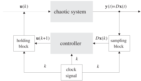
Figure 2: Structure of control system.

5 Illustrative Example

For numerical simulations the following parameters of the fractional Chua’s system (3) were chosen:

$$\alpha=10,\,\,\beta=\frac{100}{7},\,\,q=0.9,\,\,a=-1.27,\,\,b=-0.68,$$

and the following parameters (experimentally found) of controller:

$$B=\left(\begin{array}[]{ccc}1&0&0\\ 0&0&0\\ 0&0&0\\ \end{array}\right),\,\,C=\left(\begin{array}[]{ccc}0.8&0&0\\ 0&0&0\\ 0&0&0\\ \end{array}\right),\,\,D=\left(\begin{array}[]{ccc}-3.3&0&0\\ 0&0&0\\ 0&0&0\\ \end{array}\right).$$ (11)

Using the above parameters (11) the digital controller in state space form is defined as

$$u_{1}(k+1)=0.8u_{1}(k)-3.3x_{1}(k),$$ (12)

for $k=0,1,2,\dots$ The initial conditions for Chua’s circuit were $((x_{1}(0),x_{2}(0),x_{3}(0))$ = $(0.2,-0.1,-0.01)$ and the initial condition for the controller (12) was $((u_{1}(0)$ = $(0))$. The sampling period (frequency) was $T=100$ Hz.

For the computation of the fractional-order derivative in equations (4), the relations (3), (4) and properties (5), (6) were used. The length of memory was $L=10$  ($1000$ coefficients for $T=100$ Hz).

Fig. 3 shows the attractor of Chua’s circuit (3) without control. Similar behaviour was shown in work [4], where piecewise linear nonlinearity was replaced by cubic nonlinearity which yields very similar behaviour.

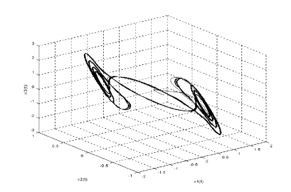
Figure 3: Strange attractor of fractional-order Chua’s system without control.

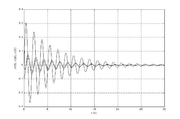
Figure 4: Controlled state variables $x_{1}(t),x_{2}(t),x_{3}(t)$.

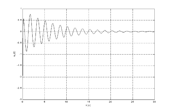
Figure 5: Control signal $u_{1}(t)$.

In Fig. 4 is shown the controlled trajectory of state variables of the fractional-order Chua’s system (4), which tends to origin asymptotically.

In Fig. 5 is shown control signal from the digital controller (12).

6 Conclusion

We have considered an example of control of chaotic fractional-order Chua’s circuit, which exhibits chaotic behaviour with total order less than three. As has been demonstrated, the idea of fractional calculus requires one to reconsider dynamic system concepts that are often taken for granted. So by decreasing the order of a system from $3$ to $2+q$ in this way, we also move from a three-dimensional system to one of infinite dimension. This system can be controlled by sampled data. The sampled data of output are sufficient for constructing the control signals in the digital controller. Digital controllers had been widely used in industry.

The conclusion of this work confirms the conclusions of the works [4], [6], [11] that there is a need to refine the notion of the order of a system which can not be considered only by the total number of differentiation. For fractional-order differential equations the number of terms is more important than the order of differentiation.

The results presented in this contribution give basis for controlling chaotic fractional-order systems. An alternative approximation of fractional-order derivative, stability investigation, and also other chaotic fractional-order system will be used in further work.

References

- [1] P. Arena, R. Caponetto, L. Fortuna and D. Porto, “Bifurcation and chaos in non-integer order cellular neural networks”, Int. J. Bifurcation and Chaos 8 (1998) 1527–1539.
- [2] L. Dorcak, “Numerical Models for Simulation the Fractional-Order Control Systems”, UEF SAV, The Academy of Sciences, Inst. of Exper. Phys., Kosice, Slovak Republic, 1994.
- [3] H. Bai-Iin, Elentary Symbolic Dynamics and Chaos in Dissipative Systems, World Scientific, Singapore, 1989.
- [4] T. T. Hartley, C. F. Lorenzo and H. K. Qammer, “Chaos on a Fractional Chua’s System”, IEEE Trans. on Circuits and Systems. Theory and Applications 42 (1995) 485–490.
- [5] H. Lenz and D. Obradovic, “Robust control of the chaotic Lorenz system”, Int. J. Bifurcation and Chaos 7 (1997) 2847–2854.
- [6] S. Nimmo and A. K. Evans, “The Effects of Continuously Varying the Fractional Differential Order of Chaotic Nonlinear Systems”, Chaos, Solitons & Fractals 10 (1999) 1111–1118.
- [7] K. B. Oldham and J. Spanier, The Fractional Calculus, Academic Press, New York, 1974.
- [8] S. Pan and F. Yin, “Optimal control of chaos with synchronization”, Int. J. Bifurcation and Chaos 7 (1997) 2855–2860.
- [9] T. S. Parker and L. O. Chua, Practical Numerical Algorithm for Chaotic Systems, Springer - Verlag, New York, 1989.
- [10] I. Petras, “The Fractional-order controllers: Methods for their synthesis and application”, J. Electrical Eng. 9-10 (1999) 284–288.
- [11] I. Podlubny, Fractional Differential Equations, Academic Press, San Diego, 1999.
- [12] T. Ushio, “Synthesis of Synchronized Chaotic Systems Based on Observers”, Int. J. Bifurcation and Chaos 9 (1999) 541–546.
- [13] T. Yang and L. O. Chua, “Control of chaos using sampled-data feedback control”, Int. J. Bifurcation and Chaos 8 (1998) 2433–2438.