The Quantum-Classical Correspondence in Polygonal Billiards

Abstract

We show that wave functions in planar rational polygonal billiards (all angles rationally related to $\pi$) can be expanded in a basis of quasi-stationary and spatially regular states. Unlike the energy eigenstates, these states are directly related to the classical invariant surfaces in the semiclassical limit. This is illustrated for the barrier billiard. We expect that these states are also present in integrable billiards with point scatterers or magnetic flux lines.

PACS numbers: 03.65.Sq, 03.65.-w, 05.45.Mt

I Introduction

The relation between wave motion in the short-wavelength regime and the corresponding ray dynamics is of fundamental importance in quantum mechanics, electromagnetics and acoustics. It has been found in quantum mechanics that the properties of the stationary solutions of the Schrödinger equation, the eigenstates $|E_{j}\rangle$ of the Hamiltonian, reflect the degree of order in the classical ray dynamics. For example, energy eigenfunctions $\langle x,y|E_{j}\rangle$ of classically integrable systems with quasiperiodic motion on invariant tori are regular, while eigenfunctions of classically chaotic systems with ergodic motion on energy surfaces are typically irregular. For generic systems, it has been conjectured [Berry77] (see [Robnik98] for a review) that in the (semi-)classical limit $\hbar\to 0$ the averaged Wigner transforms of typical energy eigenfunctions “condense” uniformly onto the underlying classical stationary objects in phase space, which are usually invariant tori, chaotic components or entire energy surfaces. In this article, however, we consider a class of systems with exotic classical invariant surfaces for which it is not clear a priori whether such a condensation scenario exists.

The classical free motion inside a planar domain ${\cal Q}$ with elastic reflection at the boundary has a constant of motion, Hamilton’s function $H=p_{x}^{2}+p_{y}^{2}+V(x,y)$. The particle’s mass is $1/2$, and $V(x,y)=0$ if $(x,y)\in{\cal Q}$ and $\infty$ otherwise. A billiard with polygonal boundary has a second constant of motion $K(p_{x},p_{y})$ if all angles $\alpha_{j}$ between sides are rationally related to $\pi$, i.e. $\alpha_{j}=m_{j}\pi/n_{j}$, where $m_{j},n_{j}>0$ are relatively prime integers [Hobson75, ZemlyakovKatok76]. However, this does not imply integrability in the sense of Liouville-Arnol^′d [Arnold78]. The Poisson bracket $\{H,K\}$ vanishes identically only if $m_{j}=1$ for all $j=1,2,\ldots$, so only rectangles, equilateral triangles, $\pi/2,\pi/4,\pi/4$-triangles, and $\pi/2,\pi/3,\pi/6$-triangles are integrable. Critical corners with $m_{j}>1$ destroy the integrability in a singular way: $\{H,K\}$ is zero everywhere in phase space except at a measure-zero set corresponding to the critical corners; the phase space is foliated by two-dimensional invariant surfaces $H,K=\mbox{constant}$ as in integrable systems, but they do not have the topology of tori. The motion is not quasiperiodic and characterized as pseudointegrable [RichensBerry81].

The quantum mechanical free wave motion with Dirichlet boundary conditions on a rational polygon barely reflects the classical pseudointegrability if only individual eigenfunctions of the Hamiltonian $\mbox{\boldmath$H$\unboldmath}=H(\mbox{\boldmath$x$\unboldmath},\mbox{\boldmath$y$\unboldmath},\mbox{\boldmath$p$\unboldmath}_{x},\mbox{\boldmath$p$\unboldmath}_{y})$ are considered. A typical eigenfunction is hard to distinguish from eigenfunctions in classically chaotic systems [BiswasJain90, BellomoUzer95, VUF95, TomiyaYoshinaga96]. It is in general not an eigenfunction of the second operator $\mbox{\boldmath$K$\unboldmath}=K(\mbox{\boldmath$p$\unboldmath}_{x},\mbox{\boldmath$p$\unboldmath}_{y})$ and has nonzero uncertainty $\Delta K=(\langle\mbox{\boldmath$K$\unboldmath}^{2}\rangle-\langle\mbox{\boldmath$K$\unboldmath}\rangle^{2})^{1/2}$, since the commutator $[\mbox{\boldmath$H$\unboldmath},\mbox{\boldmath$K$\unboldmath}]$ does not vanish. Only a subtle signature of pseudointegrability seems to be contained in individual energy eigenfunctions, namely in the distribution of zeroes of the associated Husimi function [BS99]. The closeness to the quantum mechanics of chaotic systems on the one side and to the classical dynamics of integrable systems on the other side is a first hint of an unusual quantum-classical correspondence.

A further indication pointing in this direction comes from an analogy with the metal-insulator transition of the Anderson model in three dimensions. Both kinds of systems have energy level statistics close to the semi-Poisson distribution [BGS99]. In the Anderson model, at the transition point between extended states with Wigner statistics and localized states with Poisson distributed energy levels, this intermediate statistics has its origin in the multi-fractal character of the wave functions, which are neither extended nor localized [SG91]. Analogously, a typical energy state in a rational polygon is expected to be a fractal in momentum space [BGS99], localized around an energy surface but neither extended nor localized within this surface; condensation onto a lower-dimensional invariant surface is ruled out.

As a final indication we will present a numerical study on a particular system, the barrier billiard. Instead of Wigner transforms in four-dimensional phase space, we study distributions in the two-dimensional $(H,K)$-space, where each point represents a classical invariant surface. In this context, we define condensation as $\Delta H/\langle\mbox{\boldmath$H$\unboldmath}\rangle\to 0$ and $\Delta K/\langle\mbox{\boldmath$K$\unboldmath}\rangle\to 0$ in the semiclassical limit. This ensures that mean values of the quantum operators in highly excited states can be interpreted as well-defined values of the classical constants of motion. Our central issue is to demonstrate that even though the energy states presumably do not show such a condensation there is an alternative basis of states which do so up to classically long times.

The paper is organized as follows. In Sec.II we construct the basis for general rational polygons. Its time evolution is discussed in Sec. III. In Sec. IV we illustrate our statements for the barrier billiard. We conclude with a brief summary in Sec. V and an Appendix with details on the numerical computations.

II Construction of the basis

In the following, we will introduce states with relatively small $\Delta K$ at the expense of a nonzero but also small energy uncertainty $\Delta H$. As for coherent states in the harmonic oscillator [Glauber63], we will minimize the product of the uncertainties involved. To do so, we consider the uncertainty relation

$$\Delta H\Delta K\geq\frac{1}{2}|\langle[\mbox{\boldmath$H$\unboldmath},\mbox{\boldmath$K$\unboldmath}]\rangle|\ .$$ (1)

It is an easy matter to show that the equality in (1) holds in a state $|L\rangle$ satisfying

$$(\mbox{\boldmath$H$\unboldmath}-\langle\mbox{\boldmath$H$\unboldmath}\rangle)|L\rangle=ia(\mbox{\boldmath$K$\unboldmath}-\langle\mbox{\boldmath$K$\unboldmath}\rangle)|L\rangle\ ,$$ (2)

where $i^{2}=-1$, $a$ is an arbitrary real number and $\langle\ldots\rangle=\langle L|\ldots|L\rangle$ with $\langle L|L\rangle=1$. $|L\rangle$ has to be a right eigenvector of the operator

$$\mbox{\boldmath$L$\unboldmath}=\mbox{\boldmath$H$\unboldmath}-ia\mbox{\boldmath$K$\unboldmath}\ .$$ (3)

$L$ does not commute with its adjoint. It therefore does not belong to the class of normal operators, which contains Hermitian and unitary operators as special cases. In general, the right eigenvectors of a nonnormal operator cannot be used as a basis. Instead, right and left eigenvectors together form a biorthogonal basis; see, e.g., [Wilkinson65]. In our case, however, $\langle E_{i}|\mbox{\boldmath$L$\unboldmath}|E_{j}\rangle$ is a complex-symmetric matrix due to the fact that the Hermitian matrices $\langle E_{i}|\mbox{\boldmath$H$\unboldmath}|E_{j}\rangle$ and $K_{ij}=\langle E_{i}|\mbox{\boldmath$K$\unboldmath}|E_{j}\rangle$ can be made real. Left and right eigenvectors are therefore identical and form separately a nonorthogonal basis. Furthermore, it can be shown that $\Delta H=|a|\Delta K$. In order to have equal uncertainties we choose $a=1$ (states with $a=-1$ are identical). The real and imaginary parts of the complex eigenvalues $L$ have a physical interpretation as mean energies $\langle\mbox{\boldmath$H$\unboldmath}\rangle$ and $-\langle\mbox{\boldmath$K$\unboldmath}\rangle$, respectively. Note that the classical function $H-iK$ is a constant of motion whose constant-level surfaces are the invariant surfaces.

We derive now the properties of the $|L\rangle$-states in the limit $\hbar\to 0$. Without loss of generality, we stipulate that $K$ and $K$ are homogeneous functions of the momenta of degree two, like $H$ and $H$. Starting from the expansion (see, e.g., [Brenig92, HOSW84])

$$\langle p_{x},p_{y}|i[\mbox{\boldmath$H$\unboldmath},\mbox{\boldmath$K$\unboldmath}]|x,y\rangle\langle x,y|p_{x},p_{y}\rangle=\hbar\{H,K\}+O(\hbar^{2})\ ,$$ (4)

we will exploit only the fact that the Poisson bracket $\{H,K\}$ is everywhere zero except at isolated critical points in position space. The following line of reasoning is therefore also true for integrable billiards with a finite number of magnetic flux lines or point scatterers (we have checked this for Šeba’s billiard [Seba90]). In the semiclassical regime, both sides of Eq. (4) are very small in the region ${\cal Q}\setminus{\cal C}$ excluding the union ${\cal C}$ of neighborhoods of the critical corners, the area of which shrinks to zero as $\hbar\to 0$. Manipulating Eq. (2) and restricting the integration over an $|L\rangle$-state to region ${\cal Q}\setminus{\cal C}$ gives

$$(\Delta H_{{\cal Q}\setminus{\cal C}})^{2}+(\Delta K_{{\cal Q}\setminus{\cal C}})^{2}=\langle i[\mbox{\boldmath$H$\unboldmath},\mbox{\boldmath$K$\unboldmath}]\rangle_{{\cal Q}\setminus{\cal C}}\ ,$$ (5)

with $(\Delta H_{{\cal Q}\setminus{\cal C}})^{2}=\langle(\mbox{\boldmath$H$\unboldmath}-\langle\mbox{\boldmath$H$\unboldmath}\rangle)^{2}\rangle_{{\cal Q}\setminus{\cal C}}$, etc (Note that $\langle 1\rangle_{{\cal Q}\setminus{\cal C}}<1$). The smallness of the l.h.s. of Eq. (4) carries over to both sides of Eq. (5). From this we conclude that a function $\langle x,y|L\rangle$ in region ${\cal Q}\setminus{\cal C}$ is locally either very small or can be approximated by a joint eigenfunction of both operators $H$ and $K$. Such a joint eigenfunction cannot fulfill the boundary conditions globally, otherwise the billiard would be integrable. Loosely speaking, region ${{\cal Q}\setminus{\cal C}}$ must be divided into subregions in each of which a joint eigenfunction (or a vanishing function) fulfills the boundary conditions locally. Joint eigenfunctions of neighboring subregions match smoothly, so they must have roughly the same number of nodal lines. Hence, $|L\rangle$-states have features of energy states of integrable systems: (i) the functions $\langle x,y|L\rangle$ are in some regions regular while in other regions, separated by “caustics”, vanishing; (ii) they can be labelled by two “quantum numbers” $(n_{1},n_{2})$; (iii) the eigenvalues $L=\langle\mbox{\boldmath$H$\unboldmath}\rangle-i\langle\mbox{\boldmath$K$\unboldmath}\rangle$ are regularly distributed in the complex plane. The last property holds because $\langle\mbox{\boldmath$H$\unboldmath}\rangle$ (all arguments are also valid for quantities derived from $K$) is asymptotically equal to $\langle\mbox{\boldmath$H$\unboldmath}\rangle_{{\cal Q}\setminus{\cal C}}$, which is approximately a homogeneous function of the quantum numbers of degree two due to the homogeneity of $H$. The non-relevance of $\langle\mbox{\boldmath$H$\unboldmath}\rangle_{\cal C}$ can be understood with a renormalization procedure. Going from $(n_{1},n_{2})$ to $(2n_{1},2n_{2})$, we get a new wave function with slightly larger region ${{\cal Q}\setminus{\cal C}}$ containing four times more nodal lines, and region ${\cal C}$ being a four times smaller copy of the old region ${\cal C}$. Hence, $\langle\mbox{\boldmath$H$\unboldmath}\rangle_{{\cal Q}\setminus{\cal C}}$ roughly increases by a factor of four, while $\langle\mbox{\boldmath$H$\unboldmath}\rangle_{\cal C}$ stays constant. This leads to $\langle\mbox{\boldmath$H$\unboldmath}\rangle\to\langle\mbox{\boldmath$H$\unboldmath}\rangle_{{\cal Q}\setminus{\cal C}}$ as more and more renormalization steps bring us towards the semiclassical limit.

The approximate homogeneity of $\langle\mbox{\boldmath$H$\unboldmath}\rangle_{{\cal Q}\setminus{\cal C}}$ with respect to the quantum numbers ensures that the local transitions between different joint eigenfunctions induce only a small uncertainty $(\Delta H_{{\cal Q}\setminus{\cal C}})^{2}$ of order $\langle\mbox{\boldmath$H$\unboldmath}\rangle\ll\langle\mbox{\boldmath$H$\unboldmath}^{2}\rangle$, increasing roughly by a factor of four under the action of the renormalization. The same factor is an upper bound for the increase of $(\Delta H_{\cal C})^{2}$, corresponding to a $\langle\mbox{\boldmath$H$\unboldmath}^{2}\rangle$-scaling weighted with the size of ${\cal C}$. The sum $(\Delta H)^{2}=(\Delta H_{{\cal Q}\setminus{\cal C}})^{2}+(\Delta H_{\cal C})^{2}$ therefore increases by a factor of four. Hence,

$$(\Delta H)^{2}\propto\langle\mbox{\boldmath$H$\unboldmath}\rangle\ ,\;\;(\Delta K)^{2}\propto\langle\mbox{\boldmath$K$\unboldmath}\rangle$$ (6)

in the semiclassical limit. Consequently,

$$\lim_{\hbar\to 0}\frac{\Delta H}{\langle\mbox{\boldmath$H$\unboldmath}\rangle}\to 0\ ,\;\;\lim_{\hbar\to 0}\frac{\Delta K}{\langle\mbox{\boldmath$K$\unboldmath}\rangle}\to 0\ ,$$ (7)

i.e. the $|L\rangle$-states condense onto the invariant surfaces.

III Time evolution

The time dependence of $|L\rangle$-states is non-trivial since $L$ does not commute with the Hamiltonian; $|L(t)\rangle$ is in general not an eigenstate of $L$ for $t>0$. Let us define three time scales associated with a given state $|L\rangle$ at time $t=0$: the quantum mean period, the lifetime and the classical mean free time

$$\tau_{\text{Q}}=\frac{2\pi\hbar}{\langle\mbox{\boldmath$H$\unboldmath}\rangle}\ ,\;\;\tau_{\text{L}}=\frac{2\pi\hbar}{\Delta H}\ ,\;\;\tau_{\text{C}}=\sqrt{\frac{A}{2\langle\mbox{\boldmath$H$\unboldmath}\rangle}}\ ,$$ (8)

where $A$ is the area of the billiard. From Eq. (6) we get $\tau_{\text{Q}}\ll\tau_{\text{L}}\approx\tau_{\text{C}}$, i.e. the state is quasi-stationary with a lifetime of order of the classical mean free time.

At first glance, it seems that the state fails to condense onto an invariant surface for classical long times $t\gg\tau_{\text{C}}$. However, the requirements for condensation, small relative uncertainties and constant mean values of $H$ and $K$, may persist beyond the lifetime of the state. Clearly, this is true for the relative uncertainty and the mean value of $H$ since this operator commutes with the evolution operator $\exp{(-i\mbox{\boldmath$H$\unboldmath}t/\hbar)}$. Keeping in mind that $\langle i[\mbox{\boldmath$H$\unboldmath},\mbox{\boldmath$K$\unboldmath}]\rangle$ is relatively small, we may expect that the relative uncertainty and the mean value of $K$ change slower than the state itself. To see this, we define the time scale associated with

$$\langle\mbox{\boldmath$K$\unboldmath}\rangle(t) = \langle L(t)|\mbox{\boldmath$K$\unboldmath}|L(t)\rangle$$ (9)

$$= \sum_{j,k=1}^{\infty}\langle L|E_{j}\rangle K_{jk}e^{i(E_{j}-E_{k})t/\hbar}\langle E_{k}|L\rangle\ .$$ (10)

in the same way as the lifetime in Eq. (8) as $\tau_{\text{K}}=2\pi\hbar/\Delta H_{K}$, where

$$(\Delta H_{K})^{2}=\frac{\sum_{j,k}|\langle L|E_{j}\rangle K_{jk}(E_{j}-E_{k})\langle E_{k}|L\rangle|^{2}}{2\sum_{j,k}|\langle L|E_{j}\rangle K_{jk}\langle E_{k}|L\rangle|^{2}}$$ (11)

is the mean energy difference, i.e. mean frequency difference, of the energy states involved, but in contrast to $\Delta H$ the states are weighted according to their relevance for $\langle\mbox{\boldmath$K$\unboldmath}\rangle(t)$. Two extreme cases show that definition (11) is reasonable: a diagonal matrix $K_{jk}$ gives $\Delta H_{K}=0$ whereas a uniform matrix $K_{jk}=\mbox{constant}$ gives $\Delta H_{K}=\Delta H$.

The series (9) can be expanded in orders of $t$, with $t$ much smaller than $\tau_{\text{K}}$ but with the possibility of being larger than the quantum mean period and even the lifetime. Clearly, the zeroth-order term is $\langle\mbox{\boldmath$K$\unboldmath}\rangle$. The next terms are roughly of order $\langle\mbox{\boldmath$K$\unboldmath}\rangle\Delta H_{K}t$, $\langle\mbox{\boldmath$K$\unboldmath}\rangle(\Delta H_{K}t)^{2}$, and so on. If we compare this to

$$\langle\mbox{\boldmath$K$\unboldmath}\rangle(t)=\langle\mbox{\boldmath$K$\unboldmath}\rangle+\langle i[\mbox{\boldmath$H$\unboldmath},\mbox{\boldmath$K$\unboldmath}]\rangle t/\hbar+O(t^{2})\ ,$$ (12)

we find that the order of $\tau_{\text{K}}$ can be estimated as $2\pi\langle\mbox{\boldmath$K$\unboldmath}\rangle/\langle i[\mbox{\boldmath$H$\unboldmath},\mbox{\boldmath$K$\unboldmath}]\rangle$. It follows that in the semiclassical limit $\langle\mbox{\boldmath$K$\unboldmath}\rangle(t)$ does not change relative to its initial value for classically long times $t$ below $\tau_{\text{K}}\gg\tau_{\text{C}}$, even though $|L(t)\rangle$ may differ strongly from the initial state $|L\rangle$.

Following the same line of reasoning shows that the time below which $\langle\mbox{\boldmath$K$\unboldmath}^{2}\rangle(t)$ relative to its initial value is constant scales as $\langle\mbox{\boldmath$K$\unboldmath}^{2}\rangle/\langle i[\mbox{\boldmath$H$\unboldmath},\mbox{\boldmath$K$\unboldmath}^{2}]\rangle$. Starting from Eq. (2) the following equation can be derived

$$\langle i[\mbox{\boldmath$H$\unboldmath},\mbox{\boldmath$K$\unboldmath}^{2}]\rangle-2\langle\mbox{\boldmath$K$\unboldmath}\rangle\langle i[\mbox{\boldmath$H$\unboldmath},\mbox{\boldmath$K$\unboldmath}]\rangle=2\langle(\mbox{\boldmath$K$\unboldmath}-\langle\mbox{\boldmath$K$\unboldmath}\rangle)^{3}\rangle\ .$$ (13)

With the renormalization procedure it can be shown that the asymptotic behavior of the r.h.s of this equation is bounded from above by $\langle\mbox{\boldmath$K$\unboldmath}\rangle^{2}$. Together with the already known result $\langle i[\mbox{\boldmath$H$\unboldmath},\mbox{\boldmath$K$\unboldmath}]\rangle\propto\langle\mbox{\boldmath$K$\unboldmath}\rangle$ we finally get the upper bound $\langle i[\mbox{\boldmath$H$\unboldmath},\mbox{\boldmath$K$\unboldmath}^{2}]\rangle\propto\langle\mbox{\boldmath$K$\unboldmath}^{2}\rangle$. Hence, the time scale which governs $\langle\mbox{\boldmath$K$\unboldmath}^{2}\rangle(t)$ is of the same or of larger order as $\tau_{\text{K}}$. From this we can conclude that for times smaller than $\tau_{\text{K}}$, $\Delta K(t)$ remains small if compared with $\langle\mbox{\boldmath$K$\unboldmath}\rangle(t)$. Hence, Eq. (7) holds not only for times of order $\tau_{\text{L}}\approx\tau_{\text{C}}$ but also for times much larger than $\tau_{\text{C}}$ and well below $\tau_{\text{K}}$. The condensation of $|L\rangle$-states onto invariant surfaces outlives the lifetime of the states up to classically long times.

IV Example: the barrier billiard

We illustrate all statements for the barrier billiard [Zwanzig83, HM90, Wiersig00], a rectangle with width $l_{x}$ and height $l_{y}$ and a vertical barrier of length $l_{y}/2$ placed on the symmetry line $x=l_{x}/2$; see Fig. 1(a). The billiard is not only pseudointegrable, it is also almost-integrable [Gutkin86], i.e. is composed of several copies of a single integrable sub-billiard, here the rectangle shown in Fig. 1(b). The function $K=p_{x}^{2}$ is a second constant of motion. The general formula for the genus of the invariant surfaces [RichensBerry81] gives 2, i.e. the surfaces have the topology of two-handled spheres and not that of tori (single-handled spheres).

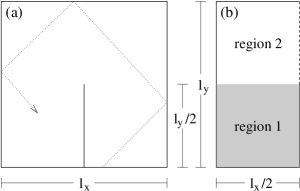
FIG. 1.: (a) Barrier billiard, rectangle with a barrier between the points $(x,y)=(l_{x}/2,0)$ and $(l_{x}/2,l_{y}/2)$. (b) Symmetry reduced system. The nontrivial wave functions fulfill Dirichlet (Neumann) boundary conditions on solid (dashed) lines.

The energy eigenfunctions are solutions of the Helmholtz equation with Dirichlet boundary conditions on the polygon. The functions are odd or even with respect to the symmetry line. The odd ones are trivial eigenfunctions of the integrable sub-billiard. We therefore deal only with the even ones, which fulfill mixed boundary conditions on the symmetry reduced polygon; see Fig. 1(b). We have calculated the solutions numerically with the mode-matching method for the parameters $\hbar=1$, $l_{x}=\pi\sqrt{8\pi}/3$, and $l_{y}=3\sqrt{8\pi}/\pi$ as described in App. 1. The statistical properties of the energy levels are found to be close to the semi-Poisson distribution [BGS99]. The energy eigenfunctions are not eigenfunctions of the operator $\mbox{\boldmath$K$\unboldmath}=\mbox{\boldmath$p$\unboldmath}^{2}_{x}$. The numerical computation of the uncertainty $\Delta K$ is explained in App. 2. Figure 2 shows that there is no trend towards vanishing relative uncertainties. This indicates that energy states of the barrier billiard do not condense onto the invariant surfaces.

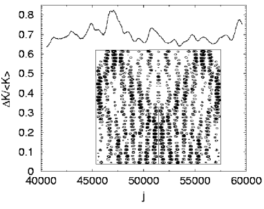
FIG. 2.: Relative uncertainty $\Delta K/\langle\mbox{\boldmath$K$\unboldmath}\rangle$ of energy states $|E_{j}\rangle$. A local Gaussian average with a variance of 200 is performed. Inset: Contour plot of the probability density associated to the 626th energy state with $E=646.03$, $\langle\mbox{\boldmath$K$\unboldmath}\rangle=135.05$ and $\Delta K=144.01$.

The nontrivial $|L\rangle$-states are also calculated with the mode-matching method. As explained in App. 3, we cannot compute as many of these states as energy states. However, even in the accessible low-energy regime our theoretical results on the semiclassical behavior of these states will be well confirmed in the following.

The regular pattern of the eigenvalues $L=\langle\mbox{\boldmath$H$\unboldmath}\rangle-i\langle\mbox{\boldmath$K$\unboldmath}\rangle$ can be most clearly seen when transformed into the real action variables of the integrable sub-billiard

$$(I_{x},I_{y})=\left(\frac{l_{x}}{2\pi}\sqrt{\langle\mbox{\boldmath$K$\unboldmath}\rangle},\frac{l_{y}}{\pi}\sqrt{\langle\mbox{\boldmath$H$\unboldmath}\rangle-\langle\mbox{\boldmath$K$\unboldmath}\rangle}\right)\ .$$ (14)

Note that the topology of the invariant surfaces in the full system rules out action-angle variables [RichensBerry81]. As can be seen from Fig. 3 the “action space” is split into two regions A and B separated by a transition region. Away from this transition region, and the lines $I_{x}=0$ and $I_{y}=0$, the eigenvalues are approximately located on regular lattices which are given by EBK-like quantization rules:

$$(I_{x},I_{y})=\left(n_{1}+\frac{3}{4},n_{2}+1\right)\hbar$$ (15)

in region A and

$$(I_{x},I_{y})=\left(\frac{n_{1}}{2}+\frac{1}{2},2n_{2}+\frac{7}{4}\right)\hbar$$ (16)

in region B with $n_{1},n_{2}=0,1,\ldots$. For example, we have $(I_{x},I_{y})\approx(6.75,37)\hbar$ for the eigenfunction of type A and $(I_{x},I_{y})\approx(21,9.7)\hbar$ for the function of type B in Fig. 4. Both types have relatively small uncertainties (see App. 4 for numerical details) and look rather regular. While type-A functions cover the billiard uniformly, apart from a localization around the critical corner, the type-B functions are restricted to the lower ($n_{1}$ odd) or upper ($n_{1}$ even) half of the billiard, bounded by a caustic-like curve.

FIG. 3.: Eigenvalues $L=\langle\mbox{\boldmath$H$\unboldmath}\rangle-i\langle\mbox{\boldmath$K$\unboldmath}\rangle$ transformed into the action space of the sub-billiard according to Eq. (14). The dotted line marks the centre of the transition region. The solid lines indicate parts of the EBK lattices defined in Eqs. (15)-(16).

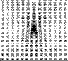
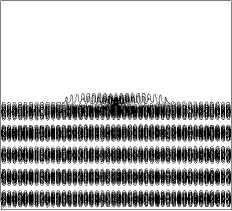
FIG. 4.: Probability density of a state $|L\rangle$ of type A (left) with eigenvalue $656.30-i64.93$ and $\Delta H=\Delta K=34.88$; type B (right) with eigenvalue $670.95-i630.52$ and $\Delta H=\Delta K=25.14$.

The eigenvalue pattern in Fig. 3 resembles strongly that of integrable systems with separatrices [RDWW96, WWD97, WWD98]. It is therefore not surprising that the statistical properties of the mean energies of $|L\rangle$-states are similar to those of energy levels of integrable systems. For example, Fig. 5 confirms that the nearest-neighbor statistics is in agreement with the Poisson distribution.

FIG. 5.: Probability density $P(s)$ of the spacing $s$ between adjacent values of the first 800 mean energies $\langle\mbox{\boldmath$H$\unboldmath}\rangle$. The data is well fitted by the Poisson distribution (dotted line).

The scaling laws (6) for the uncertainties are verified in the following way. First note that lines of constant mean energy $\langle\mbox{\boldmath$H$\unboldmath}\rangle$ are circles in the scaled action space $(2I_{x}/l_{x},I_{y}/l_{y})$. This plane can therefore be conveniently parametrized by the radial coordinate $\langle\mbox{\boldmath$H$\unboldmath}\rangle$ and the polar angle $\phi=\arctan{[(I_{y}/l_{y})/(2I_{x}/l_{x})]}$. The first scaling law holds if $(\Delta H)^{2}$ divided by $\langle\mbox{\boldmath$H$\unboldmath}\rangle$ is a function of $\phi$ alone. Figure 6 shows that this condition is well satisfied. This confirms also the second scaling law since $\Delta K=\Delta H$ and $\langle\mbox{\boldmath$K$\unboldmath}\rangle$ scales as $\langle\mbox{\boldmath$H$\unboldmath}\rangle$.

FIG. 6.: $(\Delta H)^{2}/\langle\mbox{\boldmath$H$\unboldmath}\rangle$ vs. $\phi$ with $400\leq\langle\mbox{\boldmath$H$\unboldmath}\rangle\leq 800$. The maximum lies in the transition region of action space; cf. Fig. 3.

The main features of the time dependence of $|L\rangle$-states can be observed in Figs. 7 and  8; see App. 5 for the numerical aspects. For small times $t$ around $\tau_{\text{Q}}\ll\tau_{\text{L}}\approx 26.7\tau_{\text{Q}}$, the time evolved state $|L(t)\rangle$ and the initial state $|L\rangle$ are similar; the overlap $|\langle L(t)|L\rangle|^{2}$ is close to one. For times $t\approx\tau_{\text{L}}$ both states differ considerably; the overlap is close to zero. The state has lost some of its regularity, but $\langle\mbox{\boldmath$K$\unboldmath}\rangle(t)$ and $\Delta K(t)$ stay constant up to order $\langle\mbox{\boldmath$K$\unboldmath}\rangle$ for longer times well below $\tau_{\text{K}}\approx 2736\tau_{\text{Q}}$. Interestingly, the states of type B become more uniformly distributed in configuration space in the course of time, cf. Figs. 4(b), 8(a) and (b).

FIG. 7.: Overlap $|\langle L(t)|L\rangle|^{2}$ (solid), $\langle\mbox{\boldmath$K$\unboldmath}\rangle(t)/\langle\mbox{\boldmath$K$\unboldmath}\rangle$ (dotted) and $\Delta K(t)/\langle\mbox{\boldmath$K$\unboldmath}\rangle(t)$ (dashed) for the state of type B with $L=670.95-i630.52$; cf. Fig. 4.

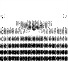
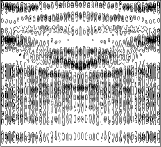
FIG. 8.: State of type B with $L=670.95-i630.52$, cf. Fig. 4, at time $t=10\tau_{\text{Q}}$ (left) and $t=\tau_{\text{L}}\approx 26.7\tau_{\text{Q}}$ (right).

V conclusion

We have formulated the quantum-classical correspondence in rational polygonal billiards in the following way: there exists a basis of quantum states with each state condensing individually onto a classical invariant surface $H,K=\mbox{constant}$ up to classically long times in the sense that the relative uncertainties $\Delta H/\langle\mbox{\boldmath$H$\unboldmath}\rangle$ and $\Delta K/\langle\mbox{\boldmath$K$\unboldmath}\rangle$ vanish in the semiclassical limit. We have presented some hints, like the analogy to the Anderson metal-insulator transition, and numerical evidence for a particular system, the barrier billiard, that the energy states do not show such a condensation. We have then introduced an alternative basis of states for which we have explicitly shown that (i) they are quasi-stationary; (ii) they condense onto the invariant surfaces up to classically long times even exceeding their lifetimes; (iii) in configuration space they show a regular nodal-line structure, possibly with caustic-like boundaries; (iv) the eigenvalues form a regular pattern in the complex plane.

Whether these states condense uniformly onto the invariant surfaces in phase space is another question. At first sight, our numerical results on the barrier billiard seem to indicate that there cannot be uniform condensation since a fraction of the states cover only one half of the configuration space. However, each such a state becomes more uniformly distributed on the invariant surface for times beyond the lifetime but remains in the neighborhood of the surface for classically long times, i.e. there can be uniform condensation after some transient time.

It is important to note that the condensation scenario holds for general rational polygonal billiards and also if the time-dependent Schrödinger equation is replaced by the wave equation used in acoustics and electromagnetics, even though the individual time scales are different.

I would like to thank M. Sieber and J. Nöckel for discussions.

Numerical computations on the barrier billiard

1 Energy states

We compute the energy eigenvalues and eigenfunctions with the mode-matching method; see, e.g.,[RichensBerry81, WSM95, ESTV96]. Let us first set $\hbar=1$ and then divide the symmetry-reduced barrier billiard in two regions as shown in Fig. 1(b): region 1 with $y\leq l$ and region 2 with $y>l$. The length of the barrier, $l$, is in our case fixed to $l_{y}/2$ but the following derivations hold also for general $0<l<l_{y}$. In region 1 we expand the wave function as

$$\Phi_{1}=\sum_{m=1}^{\infty}a_{m}\sin{(2m\pi x/l_{x})}\sin{(g_{2m}y)}$$ (17)

with

$$g^{2}_{j}(E)=E-\left(\frac{j\pi}{l_{x}}\right)^{2}.$$ (18)

This kind of expansion is nontrivial since $g_{j}$ can be imaginary and $a_{m}$ complex. By construction, the function (17) fulfills the Helmholtz equation $-\nabla^{2}\Phi_{1}=E\Phi_{1}$ with Dirichlet boundary condition on $x=0$, $y=0$, and $x=l_{x}/2$. In region 2 we take an analog function,

$$\Phi_{2}=\sum_{m=1}^{\infty}b_{m}\sin{[(2m-1)\pi x/l_{x}]}\sin{[g_{2m-1}(l_{y}-y)]}\ ,$$ (19)

which satisfies Dirichlet boundary condition on $x=0$ and $y=l_{y}$ but Neumann boundary condition on $x=l_{x}/2$. We stipulate that both functions match smoothly at $y=l$, i.e. for $0\leq x\leq l_{x}/2$ we require

$$\Phi_{1}(x,l)=\Phi_{2}(x,l)$$ (20)

and

$$\frac{\partial\Phi_{1}}{\partial y}\Biggl{|}_{(x,l)}=\frac{\partial\Phi_{2}}{\partial y}\Biggl{|}_{(x,l)}.$$ (21)

Inserting the identity

$$\sin{(2nz)}=\sum_{k=1}^{\infty}A_{nk}\sin{[(2k-1)z]}$$ (22)

for $0\leq z\leq\pi/2$ with the orthogonal matrix

$$A_{nk}=\frac{2}{\pi}\left(\frac{\sin{[(2n-2k+1)\pi/2]}}{2n-2k+1}-\frac{\sin{[(2n+2k-1)\pi/2]}}{2n+2k-1}\right)$$ (23)

into the first matching condition (20) and solving for the coefficients of $\sin{[(2n-1)\pi x/l_{x}]}$, $n=1,\ldots$, gives

$$\sum_{m=1}^{\infty}a_{m}\sin{(g_{2m}l)}A_{mn}=b_{n}\sin{[g_{2n-1}(l_{y}-l)]}\ .$$ (24)

Similarly, we get from the second matching condition (21)

$$\sum_{m=1}^{\infty}a_{m}g_{2m}\cos{(g_{2m}l)}A_{mn}=-b_{n}g_{2n-1}\cos{[g_{2n-1}(l_{y}-l)]}.$$ (25)

We now rewrite the relations (24)-(25) by using the definitions

$$\tilde{a}_{m} = a_{m}g_{2m}\cos{(g_{2m}l)},$$ (26)

$$\tilde{b}_{m} = b_{m}g_{2m-1}\cos{[g_{2m-1}(l_{y}-l)]}$$ (27)

and the real function

$$f_{m}(E,l)=\frac{\tan{(g_{m}l)}}{g_{m}}$$ (28)

as

$$\sum_{m=1}^{\infty}\tilde{a}_{m}f_{2m}(E,l)A_{mn}=\tilde{b}_{n}f_{2n-1}(E,l_{y}-l)$$ (29)

and

$$\sum_{m=1}^{\infty}\tilde{a}_{m}A_{mn}=-\tilde{b}_{n}\ .$$ (30)

The last two equations are combined to

$$\sum_{m=1}^{\infty}\tilde{a}_{m}M_{mn}=0$$ (31)

with the real matrix

$$M_{mn}(E)=[f_{2m}(E,l)+f_{2n-1}(E,l_{y}-l)]A_{mn}.$$ (32)

Equation (31) has a solution provided $\det{M(E)}=0$. Finding the energy eigenvalues $E_{i}$ is therefore equivalent to finding the zeroes of the determinant of $M$. We approximate $M$ by a $500\times 500$ matrix which is sufficient for calculating the first $100\,000$ zeroes. Figure 9 shows the determinant as a function of the energy. It is convenient to search roots numerically only between two consecutive poles. We therefore rewrite Eq. (28) using the identity [GradRyzh65]

$$-\frac{\pi}{4z}\tan{\frac{\pi z}{2}}=\sum_{n=1}^{\infty}\frac{1}{z^{2}-(2n-1)^{2}}$$ (33)

as

$$f_{m}(E,l)=-\frac{2}{l}\sum_{n=1}^{\infty}\frac{1}{E-(\frac{m\pi}{l_{x}})^{2}-(\frac{n\pi}{2l})^{2}}$$ (34)

where the summation is only over odd $n$. From this expression the poles can be easily read off. Note that the poles are not degenerate if $l^{2}/l_{x}^{2}$ and $(l_{y}-l)^{2}/l_{x}^{2}$ are irrational numbers. The interval between two given consecutive poles is divided into 400 subintervals, each assumed to contain at most a single change of sign of $\det{M}$. The bisection method is then employed in order to find each zero with an accuracy $\approx 10^{-4}$ of the mean level spacing.

FIG. 9.: Determinant of matrix $M$ in Eq. (32).

Having determined the energy levels, we get for each of them the real quantities $\tilde{a}_{m}$ and $\tilde{b}_{m}$ from Eqs. (30) and (31) and then the wavefunction (17) and (19), which we finally normalize to unity for the full billiard.

2 Uncertainties of energy states

We here determine the uncertainty $(\Delta K)^{2}=\langle\mbox{\boldmath$K$\unboldmath}^{2}\rangle-\langle\mbox{\boldmath$K$\unboldmath}\rangle^{2}$ in a given $|E_{j}\rangle$-state. We take $\Phi_{1}=\Phi_{1}(E_{j})$, $g=g(E_{j})$, and $\Phi_{2}=\Phi_{2}(E_{j})$ from Eqs. (17)-(19) to compute $K_{jj}=\langle E_{j}|\mbox{\boldmath$K$\unboldmath}|E_{j}\rangle=\langle\mbox{\boldmath$K$\unboldmath}\rangle$ from

$$K_{jj} = 2\int_{0}^{l_{x}/2}\int_{0}^{l}\Phi_{1}^{*}\left(-\frac{\partial^{2}}{\partial x^{2}}\Phi_{1}\right)dxdy$$ (35)

$$+ 2\int_{0}^{l_{x}/2}\int_{l}^{l_{y}}\Phi_{2}^{*}\left(-\frac{\partial^{2}}{\partial x^{2}}\Phi_{2}\right)dxdy\ .$$ (36)

A straightforward calculation gives

$$K_{jj} = \frac{l_{x}}{4}\sum_{m=1}^{\infty}a^{2}_{m}h_{2m}\left[l-\frac{\sin{(2g_{2m}l)}}{2g_{2m}}\right]$$ (37)

$$+ \frac{l_{x}}{4}\sum_{m=1}^{\infty}b^{2}_{m}h_{2m-1}\left[(l_{y}-l)-\frac{\sin{[2g_{2m-1}(l_{y}-l)]}}{2g_{2m-1}}\right]$$ (38)

with $a_{m}=a_{m}(E_{j})$, $b_{m}=b_{m}(E_{j})$, $g_{m}=g_{m}(E_{j})$, and $h_{m}=(m\pi/l_{x})^{2}$. Analogously, we get for $\langle\mbox{\boldmath$K$\unboldmath}^{2}\rangle=\langle\mbox{\boldmath$p$\unboldmath}^{4}_{x}\rangle$ again Eq. (37) but with $h_{m}=(m\pi/l_{x})^{4}$.

3 $|L\rangle$-states

Eigenvalues and eigenfunctions of $L$ can be computed with the procedure described in App. 1 if Eq. (18) is replaced by

$$g^{2}_{j}(L)=L-(1-i)\left(\frac{j\pi}{l_{x}}\right)^{2}$$ (39)

with complex number $L$. $M$ in Eq. (32) is then a complex matrix. Finding the complex roots of $\det{M}$ is much more cumbersome than finding real roots as in the case of the energy states. Because of this, we first compute $L$ in energy-state representation, i.e. we calculate the matrix elements $\langle E_{j}|\mbox{\boldmath$L$\unboldmath}|E_{k}\rangle=E_{j}\delta_{jk}-iK_{jk}$ with $K_{jk}=\langle E_{j}|\mbox{\boldmath$K$\unboldmath}|E_{k}\rangle$ given by Eq. (37) if $j=k$, otherwise

$$K_{jk} = \frac{l_{x}}{4}\sum_{m=1}^{\infty}a^{\dagger}_{m}a_{m}h_{2m}\left[\frac{\sin{(g^{-}_{2m}l)}}{g^{-}_{2m}}-\frac{\sin{(g^{+}_{2m}l)}}{g^{+}_{2m}}\right]$$ (40)

$$+ \frac{l_{x}}{4}\sum_{m=1}^{\infty}b^{\dagger}_{m}b_{m}h_{2m-1}\times$$ (42)

$$\left[\frac{\sin{[g^{-}_{2m-1}(l_{y}-l)]}}{g^{-}_{2m-1}}-\frac{\sin{[g^{+}_{2m-1}(l_{y}-l)]}}{g^{+}_{2m-1}}\right]$$

with $a^{\dagger}_{m}=a^{*}_{m}(E_{j})$, $a_{m}=a_{m}(E_{k})$, $b^{\dagger}_{m}=b^{*}_{m}(E_{j})$, $b_{m}=b_{m}(E_{k})$, $g^{+}_{m}=g^{*}_{m}(E_{j})+g_{m}(E_{k})$, $g^{-}_{m}=g^{*}_{m}(E_{j})-g_{m}(E_{k})$, and $h_{m}=(m\pi/l_{x})^{2}$. A LAPACK routine is used to diagonalize the complex matrix $\langle E_{j}|\mbox{\boldmath$L$\unboldmath}|E_{k}\rangle$ with $j,k\leq 1000$, giving a rough approximation to the first 800 eigenvalues of $L$. We use them as initial guesses for Newton’s method in order to find reliable approximations to the eigenvalues. Finally, we compute for each determined eigenvalue the complex quantities $\tilde{a}_{m}$ and $\tilde{b}_{m}$ from Eqs. (30) and (31) and then the normalized wavefunction (17) and (19).

4 Uncertainties of $|L\rangle$-states

The main advantage of using the mode-matching method for the $|L\rangle$-states is that we get the uncertainties $\Delta K$ and $\Delta H$ as accurately as for the energy states in App. 2. We take $\Phi_{1}=\Phi_{1}(L_{j})$, $\Phi_{2}=\Phi_{2}(L_{j})$, and $g=g(L_{j})$ from Eqs. (17), (19), and (39) to compute firstly $\langle\mbox{\boldmath$K$\unboldmath}\rangle$ starting from Eq. (35). A straightforward calculation shows that $\langle\mbox{\boldmath$K$\unboldmath}\rangle$ is given by the r.h.s. of Eq. (42) with $a^{\dagger}_{m}=a^{*}_{m}(L_{j})$, $a_{m}=a_{m}(L_{j})$, $b^{\dagger}_{m}=b^{*}_{m}(L_{j})$, $b_{m}=b_{m}(L_{j})$, $g^{+}_{m}=g^{*}_{m}(L_{j})+g_{m}(L_{j})$, $g^{-}_{m}=g^{*}_{m}(L_{j})-g_{m}(L_{j})$, and $h_{m}=(m\pi/l_{x})^{2}$. Similarly, we get for $\langle\mbox{\boldmath$K$\unboldmath}^{2}\rangle=\langle\mbox{\boldmath$p$\unboldmath}^{4}_{x}\rangle$ the same equation but with $h_{m}=(m\pi/l_{x})^{4}$; for $\langle\mbox{\boldmath$H$\unboldmath}\rangle$ we use $h_{m}=g^{2}_{m}(L_{j})+(m\pi/l_{x})^{2}$ and for $\langle\mbox{\boldmath$H$\unboldmath}^{2}\rangle$ we use $h_{m}=|g^{2}_{m}(L_{j})+(m\pi/l_{x})^{2}|^{2}$.

5 Time dependence of $|L\rangle$-states

We here compute $\langle x,y|L(t)\rangle$, $\langle L(t)|L\rangle$, $\langle\mbox{\boldmath$K$\unboldmath}\rangle(t)$ and $\langle\mbox{\boldmath$K$\unboldmath}^{2}\rangle(t)$. These expressions can be written in terms of energy states as

$$\langle x,y|L(t)\rangle = \sum_{j=1}^{\infty}e^{-iE_{j}t}\langle E_{j}|L\rangle\langle x,y|E_{j}\rangle\ ,$$ (43)

$$\langle L(t)|L\rangle = \sum_{j=1}^{\infty}e^{iE_{j}t}|\langle E_{j}|L\rangle|^{2}\ ,$$ (44)

and as in Eq. (9). The first 1400 energy states are incorporated in these sums. As in the previous sections it can be shown that $\langle E_{j}|L\rangle$ is given by the r.h.s. of Eq. (42) with $a^{\dagger}_{m}=a^{*}_{m}(E_{j})$, $a_{m}=a_{m}(L)$, $b^{\dagger}_{m}=b^{*}_{m}(E_{j})$, $b_{m}=b_{m}(L)$, $g^{+}_{m}=g^{*}_{m}(E_{j})+g_{m}(L)$, $g^{-}_{m}=g^{*}_{m}(E_{j})-g_{m}(L)$, and $h_{m}=1$. $\langle E_{j}|\mbox{\boldmath$K$\unboldmath}^{2}|E_{k}\rangle$ is also given by the r.h.s. of Eq. (42) if $j\neq k$ with $a^{\dagger}_{m}=a^{*}_{m}(E_{j})$, $a_{m}=a_{m}(E_{k})$, $b^{\dagger}_{m}=b^{*}_{m}(E_{j})$, $b_{m}=b_{m}(E_{k})$, $g^{+}_{m}=g^{*}_{m}(E_{j})+g_{m}(E_{k})$, $g^{-}_{m}=g^{*}_{m}(E_{j})-g_{m}(E_{k})$, and $h_{m}=(m\pi/l_{x})^{4}$. For $j=k$ one has to use Eq. (37).