Classical fluctuations and semiclassical matrix elements

1 Introduction

A central tool in the semiclassical analysis of chaotic systems is the Gutzwiller trace formula which relates quantal properties to classical periodic orbits [1, 2]. The extensions of Gutzwiller’s trace formula that include matrix elements in the density of states[3, 4] allow to relate distributions of quantum matrix elements and distributions of classical trajectory segments [5, 6]. Specifically, quantum fluctuations are related to fluctuations in ensembles of classical trajectory segments of length Heisenberg time. As the classical limit is approached, the Heisenberg time diverges, and the fluctuations vanish. This approach can therefore be used [5] to study the approach to ergodicity in quantum wave functions in chaotic systems. Integrable systems are not ergodic on the energy shell and therefore the fluctuations do not vanish in the semiclassical limit, as shown by Mehlig [7]. The form factors for the matrix element weighted densities of states have an additional constant contribution [6] and different behaviour in their rigidity [8]. Moreover, these relations can be used to analyse the effects near bifurcations [9] and to study localisation effects in wave functions. Beyond the static properties these can also be used to analyse the behaviour of cross sections [10, 11].

The aim here is to analyse further an observation first made in the calculation of cross sections. By Fermi’s golden rule photodissociation cross sections contain matrix elements for observables that are projections onto initial states. In this limit semiclassical arguments become suspect since the smoothness of the observable that was assumed in the derivation of the trace formulas is no longer guaranteed. However, numerical experiments indicate that even in this limit at least the widths of the distributions can be obtained from classical considerations. This behaviour of matrix elements of projection operators will be investigated further.

The behaviour of matrix elements was studied in a variety of systems, including hydrogen in magnetic fields [5, 6, 12], the bakers map[5], a perturbed cat map[13], and various billiards[7, 14]. We here use the kicked standard map as the main example[15]. The main advantage of maps is that they allow to study the semiclassical regime more easily and more deeply than continuous systems.

The outline of the paper is as follows. In section 2 we summarise information on the quantised standard map, on the semiclassical arguments that relate classical and quantal matrix elements and on the behaviour expected from random matrix theory. The numerical and analytical results on projectors are presented in section 3. We conclude with a summary and an outlook in section 4.

2 Preliminaries

2.1 The matrix element weighted density of states

In [5] we derived formulae for the width of the quantum matrix element distribution in smooth systems and proposed a formula for maps by analogy to the smooth results. To set the stage for the present investigation and to explain the origin of this formula, we here sketch the equivalent derivation for quantised maps on a finite phase space (similar to Carvalho et al[13]).

Let $U$ be the unitary operator for the time evolution, $A$ the observable and $N_{D}$ the dimension of the Hilbert space. Then there are $N_{D}$ eigenphases $\phi_{\mu}$ and eigenstates $|\mu\rangle$, so that

$$U=\sum_{\mu=1}^{N_{D}}|\mu\rangle e^{i\phi_{\mu}}\langle\mu|\,.$$ (2.1)

The matrix elements $A_{\mu}=\langle\mu|A|\mu\rangle$ are conveniently contained in the weighted density

$$\tilde{\rho}_{A}(\phi)=\sum_{\mu=1}^{N_{D}}A_{\mu}\delta(\phi-\phi_{\mu})\,.$$ (2.2)

It will be useful to work not with pure delta functions but with smeared out objects so that products are well defined. Rather than the Lorentzians or Gaussians used in previous works, the relation to finite trigonometric sums suggests to work with sinc-functions, i.e.

$$\delta_{\epsilon}(x)={1\over 2\pi}{\sin[(2N+1)x/2]\over\sin(x/2)}={1\over 2\pi}\sum_{n=-N}^{N}e^{inx}$$ (2.3)

of width $\epsilon\approx 2\pi/(2N+1)$. The advantage of this function is that the smoothed density can be expressed as a finite sum of traces of powers of the propagator, viz.

$$\rho_{A}(\phi)={1\over 2\pi}\sum_{n=-N}^{N}\sum_{\mu=1}^{N_{D}}A_{\mu}e^{in(\phi_{\mu}-\phi)}={1\over 2\pi}\sum_{n=-N}^{N}\mbox{tr\,}(A\,U^{n})\,e^{-in\phi}\,.$$ (2.4)

If $N$ is significantly smaller than $N_{D}$ some of the sinc-functions will overlap and not all individual eigenphases can be identified. Very large $N$ are impracticable from the point of view of a semiclassical approximation to be made below. Thus a natural choice is $N$ of the order of $N_{D}$ so that all eigenstates can be resolved in the mean, yet the semiclassical approximations are still reasonable.

The autocorrelation function of the smoothed density of states becomes

$$C_{A}(\theta) = {1\over 2\pi}\int_{0}^{2\pi}d\phi\,\rho_{A}(\phi-\theta/2)\rho_{A}(\phi+\theta/2)$$ (2.5)

$$= {1\over 4\pi^{2}}\sum_{n=-N}^{N}\left|\mbox{tr\,}(A\,U^{n})\right|^{2}e^{in\theta}$$ (2.6)

Up to some factors, the Fourier transform of this correlation function is the form factor. Here, since the spectrum is confined to the unit circle and a periodically continued interval in $\phi$, the form factor depends on a discrete argument only. We split off the density of states and define the form factor $K_{n}^{(A)}$ by

$$\tilde{C}_{A}(\theta)={N_{D}\over 2\pi}{1\over 2\pi}\sum_{n=-\infty}^{\infty}K_{n}^{(A)}e^{in\theta}\,.$$ (2.7)

When calculated with the smoothed density of states only the first few elements up to $N_{D}$ are included, but they do not differ from the exact ones,

$$K_{n}^{(A)}={1\over N_{D}}\left|\mbox{tr\,}(A\,U^{n})\right|^{2}\,.$$ (2.8)

As in [5], all the information needed on matrix elements is contained in the semiclassical evaluation of $K_{n}$.

Within the semiclassical approximation the trace is calculated from a stationary phase approximation to the propagator, which leads to an expression involving classical periodic orbits. Specifically,

$$\mbox{tr\,}(A\,U^{n})|_{sc}=\sum_{\gamma\in(n)}A_{\gamma}w_{\gamma}e^{iS_{\gamma}/\hbar}$$ (2.9)

where the sum extends over all distinct orbits $\gamma$ which close after $n$ iterations. $S_{\gamma}$ is the action associated with the trajectory, $w_{\gamma}$ the amplitude including phases and $A_{\gamma}$ the sum of the observable $A$ over all points of the trajectory. Of the amplitudes we need that their modulus squared equals the classical periodic orbit weight, $|w_{\gamma}|^{2}=1/|\det(1-M_{\gamma})|$, where $M_{\gamma}$ is the linearisation perpendicular to the orbit. Thus the semiclassical form factor becomes

$$|\mbox{tr\,}(A\,U^{n})|_{sc}|^{2}=\sum_{\gamma,\gamma^{\prime}\in(n)}A_{\gamma}A^{*}_{\gamma^{\prime}}w_{\gamma}w^{*}_{\gamma^{\prime}}e^{i(S_{\gamma}-S_{\gamma^{\prime}}/\hbar}\approx g\sum_{\gamma\in(n)}|A_{\gamma}|^{2}|w_{\gamma}|^{2}\,.$$ (2.10)

The neglect of the contributions from orbit pairs $(\gamma,\gamma^{\prime})$ with $\gamma\neq\gamma^{\prime}$ constitutes the diagonal approximation[16]. The factor $g$ arises from the possibility of a quantum interference of classically distinct orbits with the same action, e.g. in the case of time reversal invariant systems, where a path and its time reversed image correspond to different objects in phase space, but with the same action. Because of the quantum interference between amplitudes, it contributes with twice the classical weight, hence $g=2$. In systems without such symmetries, like the unitary ensemble, $g=1$.

The extraction of the variance of the matrix elements from the form factors proceeds as in Ref. [6]. The contributions $A_{\gamma}$ from orbits with similar period consist of two parts, one proportional to the mean of the observable and to the length of the orbit and one capturing the fluctuations, i.e. $\langle A_{\gamma}^{2}\rangle=\langle A_{\gamma}\rangle^{2}n^{2}+\alpha n$. Taking the square, averaging over orbits of similar length and exploiting the periodic orbit sum rule (which absorbs one factor of $n$) gives

$$K_{n}^{(A)}\approx g\langle A\rangle^{2}\frac{n}{N_{D}}+g\alpha\frac{1}{N_{D}}$$ (2.11)

The linear increase of the first term is the small $n$ expansion of the form factor, correct up to $n=N_{D}$ for the unitary ensemble but approximate only for the orthogonal ensemble[17]. If the mean of the observable vanishes $K_{n}^{(A)}$ is already the variance of the matrix elements and thus contained in the second term of (2.11). Since the periodic orbit sum rule is an asymptotic statement, we take $n$ as large as possible, but limited by the requirement that the diagonal approximation be reasonable and a semiclassical approximation possible. We therefore take $n=N_{D}$, the Heisenberg time.

This calculation relates only the first and second moments of classical and quantal distributions. The main aim here will be to compare the full distributions, especially in the limit of singular observables.

2.2 Connection to random matrix theory

As demonstrated in a number of studies[15, 18, 19], the short range statistical properties of quantised chaotic maps are in good agreement with those of ensembles of random matrices. So in the present context one can ask for the prediction of random matrix theory for the diagonal matrix elements. In particular, for the kind of maps and observables studied here, the relevant input is the statistics of eigenvector components. For the unitary ensembles, the distribution of real and imaginary parts can be calculated from the assumption of independent elements and the normalisation condition. For sufficiently large dimensions, this results in essentially Gaussian distributions,

$$P(x,y)=\sqrt{N_{D}\over\pi}e^{-N_{D}x^{2}}\,\sqrt{N_{D}\over\pi}e^{-N_{D}y^{2}}\,.$$ (2.12)

If $A_{\mu}=\langle\mu|A|\mu\rangle$ denotes the matrix element of $A$ with respect to the basis set, the matrix element with respect to an eigenstate $\mu$ described by the amplitudes $x_{\mu}+iy_{\mu}$ becomes

$$A=\sum_{\mu}A_{\mu}(x_{\mu}^{2}+y_{\mu}^{2})\,.$$ (2.13)

The probability density for the distribution of the matrix elements then becomes

$$P(A)=\int\delta(A-\sum_{\mu}A_{\mu}(x_{\mu}^{2}+y_{\mu}^{2}))\,\prod_{\mu=1}^{N_{D}}P(x_{\mu},y_{\mu})dx_{\mu}dy_{\mu}\,.$$ (2.14)

By the usual manipulations this becomes a Gaussian in the limit of large $N_{D}$,

$$P(A)=\sqrt{N_{D}\over 2\pi\sigma_{A}^{2}}e^{-N_{D}(A-\langle A\rangle)^{2}/2\sigma_{A}^{2}}$$ (2.15)

where

$$\langle A\rangle={1\over N_{D}}\sum_{\mu}A_{\mu}\qquad\sigma_{A}^{2}={1\over N_{D}}\sum_{\mu}A_{\mu}^{2}-\langle A\rangle^{2}$$ (2.16)

are the average and variance of the matrix elements of $A$ in the original basis.

2.3 The map

We close this section with a description of the quantum version of the kicked rotator used here. The kicking potential

$$V(\phi)=k(\cos\phi-\gamma\sin(2\phi))$$ (2.17)

gives rise to the classical map

$$p_{n+1} = p_{n}+k(\sin\phi+2\gamma\cos(2\phi))$$

$$\phi_{n+1} = \phi_{n}+p_{n+1}\,.$$ (2.18)

The parameter $k$ is the kick strength and $\gamma$ is used to break a reflection symmetry of the map. It is obviously periodic of period $2\pi$ in $\phi$. As we will study the quantum map at the case of resonance, the momentum $p$ is not unbounded but also restricted to be periodic with period $2\pi r$, where $r$ is the number of classical resonances. The parameter $\gamma$ can be used to change continuously between the cases with time reversal symmetry ($\gamma=0$) and without (we take $\gamma=1$, for intermediate behaviour see [20, 13]).

In the earlier quantum models of this map, phase space was taken to be an infinitely extended cylinder where arbitrarily large momenta were allowed, the quantum map was infinite. However, it was noted that for rational values of $\hbar$, a consistent quantisation with a finite map can be achieved. If the classical phase space extends from $-\pi r$ to $+\pi r$ in momentum and if the quantum map contains $N_{D}$ states, the effective value of Planck’s constant has a width of $2\pi$ in angle, the total phase space area is $4\pi^{2}r$. This has to be divided into $N_{D}$ quantum cells, hence $h=4\pi^{2}r/N$ or $\hbar=2\pi r/N_{D}$. We work in a momentum basis with wave functions $\langle\phi|n\rangle=e^{in\phi}/\sqrt{2\pi}$ and momentum eigenvalues $p_{n}=\hbar n=2\pi rn/N_{D}$. To avoid common factors between $r$ and $N_{D}$, we take the dimension odd, $N_{D}=2N_{1}+1$. The quantum unitary operator then has the form

$$U_{n,m}={1\over N}e^{-{i\hbar\over 4}(n^{2}+m^{2})}\sum_{j=-N_{1}}^{N_{1}}e^{-iV(\phi_{j})/\hbar-i(n-m)\phi_{j}}$$ (2.19)

where the sum extends over the points $\phi_{j}=2\pi j/N_{D}$. In order to have full symmetry over the finite momentum interval,

$$U_{n+N_{D},m}=U_{n,m+N_{D}}=U_{n,m}\,,$$ (2.20)

one should take the number of resonances to be a multiple of $4$ (if $r$ is just even translation by $N_{D}$ produces a sign change).

3 Quantum and classical matrix element distributions

In this section we compare the distributions of matrix elements in several cases. We consider the quantum kicked rotator (2.17, 2.19) and its classical counterpart (2.18). The classical kicking strength is taken to be $K=k\hbar=7$ in order to ensure complete ergodicity over the whole phase space[21]. The matrix dimension $N_{D}=201$ turns out to be sufficient to provide appropriate statistics.

3.1 Chaotic delocalised states

The observable we consider is a projection onto a subset, $I(m)$, of the unperturbed momentum basis states of length $m$,

$$A=\sum_{n\in I(m)}|n\rangle\langle n|.$$ (3.1)

Its matrix elements in the basis of the eigenstates, $\mu$, of the evolution operator (2.19) are

$$A_{\mu}=\langle\mu|A|\mu\rangle=\sum_{n\in I(m)}|\langle\mu|n\rangle|^{2}.$$ (3.2)

The projection covers a fraction $p=m/N_{D}$ of the phase space both quantum mechanically and classically.

Due to normalisation of the eigenstates the mean value of $A_{\mu}$ is $\langle A\rangle=p=m/N_{D}$. The second moment, $\langle{A^{2}}\rangle$, is defined as

$$\langle{A^{2}}\rangle=\frac{1}{N_{D}}\sum_{\mu}\,\sum_{k,l\in I(m)}|\langle\mu|k\rangle|^{2}|\langle\mu|l\rangle|^{2}.$$ (3.3)

which for $m\ll N_{D}$ can be calculated using the assumptions of random matrix theory to give

$$\langle{A^{2}}\rangle=p^{2}+g\frac{1}{N}p\,,$$ (3.4)

where $g=1$ ($g=2$) for the case of unitary (orthogonal) symmetry. Hence the variance is simply $\sigma^{2}_{A}=gp/N$.

If $m$ is sufficiently broad, $m\gg 1$, we may easily compare the distribution of these quantum matrix elements to that of the classical distribution which, in the limit $N>m\gg 1$ is essentially a Gaussian (2.15, 2.16). For the classical observable the mean and the fluctuating part can be calculated using a random–walk analogue due to the rapid decay of correlations between steps,

$$\langle A\rangle=p=m/N_{D},\qquad\alpha=p(1-p).$$ (3.5)

The classical fluctuations in the limit of $p\ll 1$ are related to the quantum variance [5]

$$\sigma_{A}^{2}=g\frac{1}{N}\alpha\,.$$ (3.6)

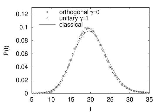
Fig. 1: Distribution of the matrix elements $A_{\mu}$ with $t=N_{D}A_{\mu}$. The orthogonal symmetry ($\gamma=0$) has been rescaled according to (3.7). The continuous curve is the binomial distribution as given in (3.8). The parameters are: $N_{D}=201$ and $m=20$.

Fig. 1 clearly demonstrates that the classical and the quantum distributions are indeed very similar when the quantum kicked rotator is used in the unitary symmetry ($\gamma=1$). In the figure we also plotted the distribution of matrix elements for $\gamma=0$, i.e. for the orthogonal case. In the latter case we adopted a rescaling according to the symmetry factor (3.6)

$$\sigma^{2}_{A}(\gamma=0)=g\,\sigma^{2}_{A}(\gamma=1).$$ (3.7)

where the $g$–factor ($g=2$), as in (2.10, 2.11, 3.4, 3.6) accounts for the fact that in the orthogonal symmetry the orbitals and their time reversed counterparts are indistinguishable. Results on the transition between the two ensembles can be found in Blümel and Smilansky [20] and in Carvalho et al. [13]

In fact one can look at the variance of the observable and compare it to the mean value for different values of $m/N$ and compare with the classical predictions. In Fig. 2 it is demonstrated that indeed for a wide range of $m$ for a fixed value of $N_{D}=201$ the behaviour of the variance is the same as presented also in Fig. 1.

Fig. 2: Quantum versus semiclassical variance of $A_{\mu}$ as a function of its mean value $\langle A\rangle=m/N_{D}$. The classical curve is $\alpha N$ (3.5). We have used $N_{D}=201$.

3.2 Singular observables

As the width of the projector, $m$, becomes smaller the assumption of an observable that is smooth on the scale of Planck’s constant is not satisfied anymore. Nevertheless, the data of Fig. 2 show that the variances are still in agreement with the semiclassical predictions. The full distribution, however, cannot remain Gaussian for $m$ approaching one, neither classical nor quantal. On the quantum side, the distribution becomes exponential for the unitary ensemble and a Porter Thomas distribution $P(t)={e^{-t/2}}/{\sqrt{2t}}$ for the orthogonal ensemble. The classical distribution, in the case of strong chaos, is a binomial distribution, i.e. the probability to hit the support of the observable $k$-times in $N_{D}$ trials is

$$W_{k}(N_{D})={N_{D}\choose k}p^{k}(1-p)^{N_{D}-k},$$ (3.8)

where $p=m/N_{D}$. From (3.8) $\langle A\rangle=Np=m$ and $\sigma^{2}_{A}=N\alpha=Np(1-p)$. The limit of $m$ approaching $1$ and diverging $N_{D}$ is the Poisson limit of the binomial distribution: for $p\to 0$ while $N_{D}\to\infty$ so that $pN=m$ is fixed the above distribution reduces to

$$P_{k}=\frac{m^{k}}{k!}e^{-m}\,,$$ (3.9)

with a clearly non-exponential dependence on $k$.

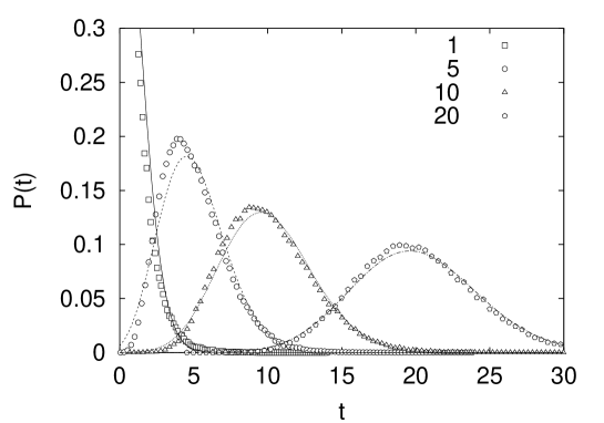
Fig. 3: Distribution of the matrix elements $A_{\mu}$ with $t=N_{D}A_{\mu}$ for the case of unitary symmetry ($\gamma=1$) with $m=1$, 5, 10, and 20. The continuous curves are the classical binomial distributions (3.8). We have used $N_{D}=201$.

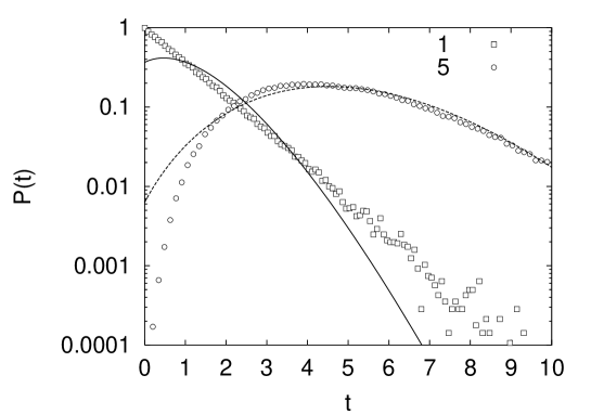
Fig. 4: Distribution of the matrix elements $A_{\mu}$ with $t=N_{D}A_{\mu}$ for the case of unitary symmetry ($\gamma=1$) with $m=1$, 5, compared to the classical binomial distributions (3.8). We have used $N_{D}=201$.

Fig. 3 shows the change of the distribution of matrix elements, $A_{\mu}$, for different values of $m$ and fixed $N_{D}=201$. The histograms nicely follow the classical distribution for large $m$. To highlight the differences for smaller values we show in Fig. 4 the cases $m=1$ and $m=5$ on a semi-logarithmic plot. The exponential distribution of the quantum matrix elements is clearly visible as is the strongly non-Gaussian behaviour of the classical distribution. The enhanced return probability in the orthogonal case and the singular behaviour of the Porter Thomas distribution give result in more pronounced differences between classical and quantal distributions than in the unitary ensemble. For instance, the distributions for $m=5$ in Fig. 5 for orthogonal symmetry show larger differences than the corresponding ones in Fig. 3 for the unitary ensemble.

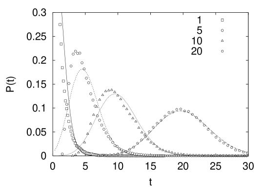
Fig. 5: Distribution of the matrix elements $A_{\mu}$ with $t=N_{D}A_{\mu}$ for the case of orthogonal symmetry ($\gamma=0$) with $m=1$, 5, 10, and 20. The continuous curves are the classical binomial distributions (3.8). The numerical data have been rescaled according to (3.7). We have used $N_{D}=201$.

3.3 Matrix element distributions near bifurcations

The previous sections have shown that while it is not always possible to obtain the full distribution of matrix elements from the classical distributions, at least the mean and the variance come out reliably. This opens the possibility to study also the distributions in situations where the assumptions of random matrix theory are not satisfied anymore, specifically in systems with mixed phase space[22] or near bifurcations of classical orbits[9, 23]. To illustrate the kind of behaviour that has to be expected near a bifurcation we consider an observable that is localised in a strip of width $2\pi/N$ around the the position of the bifurcation, $p=2\pi$. Near the bifurcation the probability to stay in this box is enhanced and so will be the contribution of this state to the matrix elements. It is thus useful to compare directly the classical and quantal probabilities to return to this box. Therefore, we compare $P_{cl}$, the classical probability for trajectories that start in the strip and return after $N$ steps and $P_{qm}=\mbox{tr\,}(A\,U^{N})$ (Ref. [24]). As can be seen from Fig. 6 both quantities show a qualitatively similar behaviour, with a rapid increase near to and a slower decline further above the bifurcation point. However, the maxima are shifted in a characteristic fashion and the scaling with $N$ is different[24].

Fig. 6: Classical and quantum return probability to the neighbourhood of bifurcation above $K=4\pi$ for $N_{D}=101$

4 Conclusions

The semiclassical theory used in Ref. [5] to relate matrix elements and classical trajectory segments requires the observable to be smooth on scales of Planck’s constant. Nevertheless, the examples discussed here show that this relation seems to hold all the way down to singular observables like projection operators onto single states. Quantum effects are always present through the symmetry factor $g$, but they are enhanced for singular observables where the form of the distribution and thus in particular the higher moments are different from what could be expected classically. Nevertheless, the possibility to analyse the second moment semiclassically should be helpful in analysing quantum chaos in systems with mixed phase spaces or near bifurcations.

References

- [1] M. C. Gutzwiller, Chaos in Classical and Quantum Mechanics, Springer New York, 1990
- [2] H.J. Stöckmann, Quantum Chaos: an introduction, Cambridge University Press, Cambridge 1999.
- [3] M. Wilkinson, J. Phys. A 20 (1987), 2415, 21 (1988), 1173
- [4] B. Eckhardt, S. Fishman, K. Müller and D. Wintgen, Phys. Rev. A 45 (1992), 3531
- [5] B. Eckhardt, O. Agam, S. Fishman, J. Keating, J. Main and K. Müller, Phys. Rev. E 52 (1995), 5893
- [6] B. Eckhardt and J. Main, Phys. Rev. Lett. 75 (1995), 2300.
- [7] B. Mehlig, Phys. Rev. E 59 (1998), 390
- [8] B. Eckhardt, Physica D 109 (1997), 53
- [9] I. Varga, P. Pollner and B. Eckhardt, Ann. Phys. (Leipzig) 8 (1999), SI265.
- [10] B. Eckhardt, S. Fishman and I. Varga, preprint
- [11] B. Eckhardt, P. Pollner and I. Varga, submitted to Physica E.
- [12] D. Boosé, J. Main, B. Mehlig, K. Müller, Europhys. Lett. 32 (1995), 295
- [13] T.O. Carvalho, J.P. Keating and J.M. Robbins, J. Phys. A 31 (1998), 5631
- [14] A. Bäcker, R. Schubert, P. Stifter, Phys. Rev. E 57 (1998), 5425 58 (1998), 5192E
- [15] F. M. Izrailev, Phys. Rep. 196 (1990), 299
- [16] M.V. Berry, Proc. R. Soc. (London) A400 (1985), 229
- [17] F. Haake, Quantum signatures of classical chaos, Springer, New York, 1992
- [18] T. Guhr, A. Müller-Groeling, H.A. Weidenmüller, Phys. Rep. 29 (1998), 190
- [19] O. Bohigas, Chaos and quantum physics, M.J. Giannoni, A. Voros and J. Zinn-Justin (eds), North Holland Amsterdam, 1990, 87
- [20] R. Blümel and U. Smilansky, Phys. Rev. Lett. 69 (1992), 217.
- [21] B.V. Chirikov and D.L. Shepelyansky, Phys. Rev. Lett. 82 (1999), 528.
- [22] B. Mehlig, K. Müller and B. Eckhardt, Phys. Rev. E 59 (1998), 5272
- [23] P. Pollner and B. Eckhardt, preprint
- [24] P. Pollner, I. Varga and B. Eckhardt, in preparation.