The lattice structure of
Chip Firing Games
Matthieu Latapy and Ha Duong Phan 

Abstract: In this paper, we study a classical discrete dynamical system, the Chip Firing Game, used as a model in physics, economics and computer science. We use order theory and show that the set of reachable states (i.e. the configuration space) of such a system started in any configuration is a lattice, which implies strong structural properties. The lattice structure of the configuration space of a dynamical system is of great interest since it implies convergence (and more) if the configuration space is finite. If it is infinite, this property implies another kind of convergence: all the configurations reachable from two given configurations are reachable from their infimum. In other words, there is a unique first configuration which is reachable from two given configurations. Moreover, the Chip Firing Game is a very general model, and we show how known models can be encoded as Chip Firing Games, and how some results about them can be deduced from this paper. Finally, we introduce a new model, which is a generalization of the Chip Firing Game, and about which many interesting questions arise.

Keywords: Discrete Dynamical Systems, Chip Firing Games, Lattice, Sand Pile Model, Convergence.

1 Preliminaries

A CFG (Chip Firing Game) [BLS91] is defined over a (directed) multigraph $G=(V,E)$, called the support or the base of the game. A weight $w(\nu)$ is associated with each vertex $\nu\ \in\ V$, which can be regarded as the number of chips stored at the site $\nu$. The CFG is then considered as a discrete dynamical system with the following rule, called the firing rule: a vertex containing at least as many chips as its outgoing degree (its number of outgoing edges) transfers one chip along each of its outgoing edges. This rule can be applied in parallel (every vertex which verifies the condition is fired at each step, see Figure 1) or in sequential (one vertex among the possible ones is fired, see Figure 2). We can already observe a few points about the example : first, the total number of chips is constant, which is obviously true for any CFG. Moreover, the example reaches a state where no firing is possible. Such a state is called a fixed point of the CFG. Notice that there exists CFGs with no fixed point. In our example, it seems that the third vertex (the one at the bottom) plays an important role, as a collector. Finally, if we fire one vertex at each step, like in Figure 2, then we may have to choose at some steps between two different vertices. It is known from [Eri93] that we will obtain a unique fixed point (if any): the CFGs are strongly convergent games. This means that either a CFG reaches a fixed point, and then this point does not depend on the choices of the vertices for firing, or the CFG has no fixed point. Indeed, we have already seen that the two cases occur, and we will explain more deeply in the following when each case occurs.

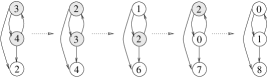
Figure 1: An example of parallel CFG. The weight of each vertex is indicated, and the shaded vertices are the ones which can be fired.

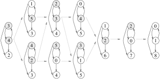
Figure 2: An example of sequential CFG. The weight of each vertex is indicated, and the shaded vertices are the ones which can be fired.

If we consider an arbitrary numbering of the vertices from $1$ to $k$, we can obtain a description of a CFG with the $k\times k$ matrix $M=(a_{ij})$ where $a_{ii}$ is the number of outgoing edges from the vertex numbered $i$, and $-a_{ij}$ is the number of edges from the vertex $j$ to the vertex $i$. The values of the other elements of the matrix are $0$. This matrix is known as the laplacian matrix of the support of the CFG [BLS91]. For example, for the CFG given in Figure 1, $k=3$ and if we order the vertices from the top to the bottom, we obtain :

$$M=\left(\begin{array}[]{ccc}2&-1&0\\ -1&2&0\\ -1&-1&0\end{array}\right).$$

The product of $M$ with a vector $v=\mbox{${}^{t}$}(v_{1},\dots,v_{k})$ gives a vector $v^{\prime}=\mbox{${}^{t}$}(v^{\prime}_{1},\dots,v^{\prime}_{k})$ such that $v^{\prime}_{i}$ is (the opposite of) the variation of the number of chips at vertex number $i$ if we fire $v_{j}$ times vertex $j$, for all $1\leq j\leq k$. Back to our example, let us consider $v=\mbox{${}^{t}$}(1,2,0)$. We have $M\times v=\mbox{${}^{t}$}(0,3,-3)$. This codes the variation in the weight of each vertex when we fire once the first vertex and twice the second: the weight of the first vertex is the same as before, while the weight of the second is decreased by $3$ and the weight of the last vertex is increased by $3$. A sink in a graph is a vertex such that there is no edge from it to any other vertex. In the following, we will order the vertices of a graph such that its sinks are the last vertices. Therefore, if this graph has $m$ sinks, then the $m$ last columns of its laplacian matrix contain only $0$.

CFGs are widely used in theoretical computer science, in physics and in economics. For example, CFGs model distributed behaviours (such as dynamical distribution of jobs over a network [Hua93, DKTR95]), combinatorial objects (such as integer partitions [GK93, Bry73] and others [CR00]). In physics, it is manly studied as a paradigm for so called Self Organised Criticality, an important area of research [BTW87, LMMP98, MN99]. It was also proved in [GM97] that (infinite) CFGs are Turing complete , which shows the potential complexity of their behaviours. However, we will prove in the following that the set of possible configurations for a CFG is strongly structured. To acheive this, we will mainly use order theory. A partially ordered set (or poset) is a set $P$ equipped with a reflexive ($x\leq x$), transitive ($x\leq y$ and $y\leq z$ implies $x\leq z$) and antisymetric ($x\leq y$ and $y\leq x$ implies $x=y$) binary relation $\leq$. A lattice is a poset such that two elements $a$ and $b$ admit a least upper bound (called supremum of $a$ and $b$ and denoted by $\sup(a,b)$) and a greatest lower bound (called infimum of $a$ and $b$ and denoted by $\inf(a,b)$). The element $\sup(a,b)$ is the smallest element among the elements greater than both $a$ and $b$. The element $\inf(a,b)$ is defined dually. For more details, see for example [DP90]. The fact that the set of configurations of a dynamical system naturally ordered is a lattice implies some important properties, such as convergence. Moreover this convergence is very strong in the following sense: for two configurations of the system, there exists a unique first congiguration obtained from them, and every configuration which can be obtained from both of them can be obtained from this first one.

In the following, we will suppose (without loss of generality) that the vertices of any graph are totally ordered, hence we will index them with integers. We suppose that this ordering is such that the sinks of the CFG (i.e. the vertices with no outgoing edges) have the greatest indices. Then, a configuration of a CFG is defined by a vector $c=(c_{1},\dots,c_{k})$ such that $c_{i}$ is the weight of the $i$-th vertex. A CFG defined over $G=(V,E)$ evolves from an initial configuration, and the set of all configurations reachable from the initial one is called the configuration space of the CFG. This set is equipped with a relation, called the successor relation, induced by the firing rule: $a\longrightarrow b$ if and only if the configuration $b$ can be obtained from the configuration $a$ by firing one vertex of the CFG. In other words, $a\longrightarrow b$ if there is one vertex $\nu$ in $V$ such that for all $v\in V,v\not=\nu$: $b_{v}=a_{v}+|\{(\nu,v)\in E\}|$ and $b_{\nu}=a_{\nu}-d^{o}_{+}(\nu)+|\{(\nu,\nu)\in E\}|$ The aim of this paper is mainly the study of this configuration space and of this relation, which gives deep insight about the behaviour of CFGs.

It will appear that a special class of CFGs play a central role for our study. The supports of these CFGs do not have any closed component :

Definition 1 (Closed Component)

A closed component of a multigraph $G$ is a nontrivial (more than one element) subset $S$ of the set of the vertices of $G$ such that

• there exists a path from any element of $S$ to any other element of $S$ ($S$ is a nontrivial strongly connected component), and

• there is no outgoing edge from one element of $S$ to a vertex of $G$ which is not in $S$ ($S$ is closed).

It is clear that the (support of the) CFG in Figure 1 has no closed component, since its unique nontrivial strongly connected component is composed of the two topmost vertices, and there is an edge from this component to the third vertex, which is a sink. Let us recall that when a chip arrives to such a sink, it can never go out. Notice that a closed component behaves as a sink, since it also has this property. We will discuss more deeply this analogy in the following. Continuing with our example, if we delete this vertex then the graph is reduced to a closed component, and we can notice that the obtained CFG has no fixed point.

2 CFG with no closed component

In this section, we will show an important lemma which allows the study of the special case where all the strongly connected components of the support of the game have at least one outgoing edge, i.e. an edge from one vertex in the component to a vertex outside the component. This means that the support of the game has no closed component. We show that in this case the successor relation of the CFGs induces an order over the configuration spaces. Then, we extend the usual definition (see for example [Eri93, BLS91]) of shot vectors and we establish the lattice structure of the configuration spaces of CFGs.

Let $G=(V,E)$ be the support multigraph of a CFG. Consider $G^{\prime}$ the quotient graph with respect to the (non closed) strongly connected components: the vertices of $G^{\prime}$ are the strongly connected components of $G$ and $C\longrightarrow D$ in $G^{\prime}$ if and only if there are vertices $a$ and $b$ of $G$ such that $a\in C$, $b\in D$, and $a\longrightarrow b$ in $G$. The quotient graph $G^{\prime}$ is obviously a directed acyclic graph.

We have the following lemma:

Lemma 1

Let us consider a non closed strongly connected component $C$. Starting from a configuration $a$ there is no nonempty sequence of firings of vertices in $C$ such that the configuration $a$ is reached again.

Proof: Suppose there is a nonempty sequence of firings of vertices in $C$ which generates a cycle in the configuration space. Then, denote by $v$ the first fired vertex. Likewise, denote by $v^{\prime}$ a vertex in $C$ such that there is a vertex $v^{\prime\prime}$ in a strongly connected component $D\not=C$ such that $v^{\prime}\longrightarrow v^{\prime\prime}$. Since $v$ and $v^{\prime}$ belong to the same strongly connected component $C$, there is a path from $v$ to $v^{\prime}$ in $G$:

$$v=v_{0}\longrightarrow v_{1}\longrightarrow v_{2}\longrightarrow\dots\longrightarrow v_{k}=v^{\prime}\longrightarrow v^{\prime\prime}.$$

After the firing of $v=v_{0}$, the weight of $v_{1}$ is increased by at least one, hence there must be a firing of $v_{1}$ in order to complete the cycle in the configuration space. Likewise, we have to fire $v_{2}$, $\dots$, $v_{k}$. But the firing of $v_{k}=v^{\prime}$ transfers one chip from $C$ to $D$, which can obviously never come back by firing only vertices in $C$. Hence we can not complete the cycle in the configuration space, and we reach a contradiction.

This lemma implies that if we only fire vertices which are not in a closed component, then we can not have any cycle of configurations. Therefore, we deduce that if all the strongly connected components which have no outgoing edge are trivial (they contain only one vertex), i.e. there is no closed component, then the configuration space of the whole CFG contains no cycle, and so it is a poset:

Theorem 1

The configuration space of a CFG with no closed component is partially ordered by the reflexive and transitive closure of the successor relation.

Moreover, we know from [Eri93] that the CFGs are strongly convergent games. In other words, either a CFG does not converge at all, either all the sequences of firings from one configuration $a$ to another one $b$ have equal length. Given such a sequence $p$, we denote by $|p|_{i}$ the number of applications of the firing rule to the $i$-th vertex during the sequence. Let us first prove the following result:

Lemma 2

Given a CFG with no closed component, if, starting from the same configuration, two sequences of firings $s$ and $t$ lead to the same final configuration, then:

$$|s|_{i}=|t|_{i}\mbox{ for each vertex }i.$$

Proof: Let $G=(V,E)$ be the support of this CFG and let $n=|V|$. Suppose that there exist two configurations $a$ and $b$ of this CFG such that there are two different sequences of firings $s$ and $t$ from $a$ to $b$ which do not satisfy the condition of the claim. Let us denote by $\sigma$ the vector $(|s|_{1},|s|_{2},\dots,|s|_{n})$ and by $\tau$ the vector $(|t|_{1},|t|_{2},\dots,|t|_{n})$. Let $M=(a_{ij})_{1\leq i,j\leq n}$ be the laplacian matrix of $G$. Recall that $-a_{ji}$ is equal to the number of edges from $i$ to $j$ in $G$, and $a_{ii}=\sum_{\stackrel{{\scriptstyle 1\leq j\leq n}}{{j\not=i}}}-a_{ji}$. We know that $M\cdot\sigma=a-b\mbox{ and }M\cdot\tau=a-b$, which implies $M\cdot(\sigma-\tau)=0.$ Let us recall that the sinks of $G$ are the last vertices $m+1,\ldots,n$ where $n-m$ is the number of sinks of $G$ and so the matrix $M$ has the following form:

$$M=\left(\begin{array}[]{ccccccc}a_{11}&a_{12}&...&a_{1m}&0&...&0\\ a_{21}&a_{22}&...&a_{2m}&0&...&0\\ ...&...&...&...&0&...&0\\ a_{m1}&a_{m2}&...&a_{mm}&0&...&0\\ a_{(m+1)1}&a_{(m+1)2}&...&a_{(m+1)m}&0&...&0\\ ...&...&...&...&0&...&0\\ a_{n1}&a_{n2}&...&a_{nm}&0&...&0\end{array}\right).$$

Remark also that for any sink $i$ (i.e. $m+1\leq i\leq n$), $|s|_{i}=|t|_{i}=0$. Let us denote by $\sigma^{\prime}$ the vector $(|s|_{1},\ldots,|s|_{m})$, by $\tau^{\prime}$ the vector $(|t|_{1},\ldots,|t|_{m})$, by $M^{\prime}$ the matrix $(a_{ij})_{1\leq i,j\leq m}$ and by $l_{i}$ the $i$-th line of $M^{\prime}$: $l_{i}=(a_{i1},\ldots,a_{im})$. We have $M\cdot(\sigma-\tau)=0$, which implies that $M^{\prime}(\sigma^{\prime}-\tau^{\prime})=0$, so $det(M^{\prime})=0$ (since $\sigma\not=\tau$, and so $\sigma^{\prime}\not=\tau^{\prime}$) and then there exists $m$ integers $k_{1},\ldots,k_{m}$ such that $k_{1}l_{1}+\dots+k_{m}l_{m}=(0,\ldots,0)$.

Let $i_{1}$ be an index such that $|k_{i_{1}}|$ is maximal between $|k_{1}|,\ldots,|k_{m}|$. Notice that $i_{1}$ is not a sink since $i\leq m$. Without loss of generality, we can suppose that $k_{i_{1}}>0$. Let us consider the $i_{1}$-th column of $M^{\prime}$; we have the following inequality:

$$k_{i_{1}}a_{i_{1}i_{1}}=k_{i_{1}}\sum_{\stackrel{{\scriptstyle j\not=i_{1}}}{{1\leq j\leq n}}}-a_{ji_{1}}\geq k_{i_{1}}\sum_{\stackrel{{\scriptstyle j\not=i_{1}}}{{1\leq j\leq m}}}-a_{ji_{1}}=\sum_{\stackrel{{\scriptstyle j\not=i_{1}}}{{1\leq j\leq m}}}-k_{i_{1}}a_{ji_{1}}\geq\sum_{\stackrel{{\scriptstyle j\not=i_{1}}}{{1\leq j\leq m}}}-k_{j}a_{ji_{1}}.$$

Moreover, by definition of $k_{j}$, we have $k_{i_{1}}a_{i_{1}i_{1}}=\sum_{\stackrel{{\scriptstyle j\not=i_{1}}}{{1\leq j\leq m}}}-k_{j}a_{ji_{1}}$, and so the inequalities above actually are equalities. Therefore:

$$\left\{\begin{array}[]{p{1cm}}\begin{minipage}{28.45274pt}$$\sum_{\stackrel{{\scriptstyle j\not=i_{1}}}{{1\leq j\leq n}}}-a_{ji_{1}}=\sum_{\stackrel{{\scriptstyle j\not=i_{1}}}{{1\leq j\leq m}}}-a_{ji_{1}}$$\end{minipage}\\ \begin{minipage}{28.45274pt}$$k_{j}a_{ji_{1}}=k_{i_{1}}a_{ji_{1}}\mbox{ for all }1\leq j\leq m$$\end{minipage}\end{array}\right.$$

which means that there is no edge from $i_{1}$ to any sink of $G$ and for every $j$, $i_{1}\rightarrow j$ in $G$ implies $k_{j}=k_{i_{1}}$.

Let us now consider a path from $i_{1}$ to a sink $i_{1}\rightarrow i_{2}\ldots\rightarrow i_{r}\rightarrow p$ (notice that such a path always exists since $G$ has no closed component). The argument above says that $k_{i_{1}}=k_{i_{2}}=\ldots=k_{i_{r}}$ and that there is no edge from $i_{1},i_{2},\ldots,i_{r}$ to any sink. But $p$ is a sink and $i_{r}\rightarrow p$ is a edge in $G$, so we have a contradiction. The proof is then complete.

This lemma allows us to define the shot vector $k(a,b)$ of two configuration $a$ and $b$ if $b$ can be obtained from $a$ in a CFG: $k(a,b)=(k_{1}(a,b),\ldots,k_{n}(a,b))$ where $k_{i}(a,b)$ is the number of firings of vertex $i$ to obtain $b$ from $a$. Let us denote by $|k(a,b)|$ the sum $\sum_{i=1}^{i=n}k_{i}(a,b)$, which is in fact the number of firings needed to obtain $b$ from $a$. If $a$ and $b$ are two configurations obtained from the same configuration $O$, we order $k(O,a)\leq k(O,b)$ if $\forall i$ $k_{i}(O,a)\leq k_{i}(O,b)$. Moreover, if $a\geq b$, it is clear that $k(O,b)=k(O,a)+k(a,b)$. Let us give here a useful result about the shot vectors:

Lemma 3

Let $a$ and $b$ be two configurations obtained from the same one $O$ such that there exists an index $j$ such that $k_{j}(O,a)\leq k_{j}(O,b)$ and $\forall j^{{}^{\prime}}\neq j,k_{j^{{}^{\prime}}}(O,a)\geq k_{j^{{}^{\prime}}}(O,b)$. If it is possible to fire the vertex $j$ of $b$, then it is also possible to fire $a$ at the same vertex.

Proof: Knowing that the necessary and sufficient condition to fire the vertex $j$ of $b$ is $b_{j}\geq v_{j}$, where $v_{j}$ is the outgoing degree of $j$, let us consider $a_{j}$:

$a_{j}$	$=$	$O_{j}-k_{j}(O,a)v_{j}+\sum_{i\rightarrow j\in G}k_{i}(O,a)$
	$\geq$	$O_{j}-k_{j}(O,b)v_{j}+\sum_{i\rightarrow j\in G}k_{i}(O,b)$
	$=$	$b_{j}$
	$\geq$	$v_{j}$.

So, it is possible to fire the vertex $j$ of $a$, which proves the result.

We can now characterize the order between all the configurations obtained from the initial one $O$ in a CFG by comparing their shot vectors as follows:

Theorem 2

If $a$ and $b$ are two configurations obtained from the same configuration $O$ of a CFG , then:

$$a\geq b\Longleftrightarrow k(O,a)\leq k(O,b).$$

Proof: If $a\geq b$ then $k(O,b)=k(O,a)+k(a,b)\geq k(O,a)$. Let us now assume that $k(O,a)\leq k(O,b)$ and consider two sequences of firings, one from $O$ to $a$ and the other from $O$ to $b$:

$$O=c_{0}\rightarrow c_{1}\rightarrow\ldots\rightarrow c_{r}\rightarrow a$$

$$O=d_{0}\rightarrow d_{1}\rightarrow\ldots\rightarrow d_{s}\rightarrow b.$$

We will construct step by step a sequence of firings $a\rightarrow e_{1}\rightarrow\ldots\rightarrow e_{t}\rightarrow b$, showing that $a\geq b$. Knowing that $(0,0,\ldots,0)=k(O,O)\leq k(O,a)\leq k(O,b)$, there exists a first configuration $d_{i}$ ($i\geq 1$) on the path from $O$ to $b$ such that $k(O,d_{i})\not\leq k(O,a)$ and $k(O,d_{i-1}\leq k(O,a)$. Let $j$ be the vertex fired during the transition $d_{i-1}\rightarrow d_{i}$. We have $k_{j^{\prime}}(O,d_{i-1})=k_{j^{\prime}}(O,d_{i})$ for all $j^{\prime}\not=j$ and $k_{j}(O,d_{i-1})+1=k_{j}(O,d_{i})$. Since $k(O,d_{i-1})\leq k(O,a)$, $k_{j^{\prime}}(O,d_{i})\leq k_{j^{\prime}}(O,a)$ for all $j^{\prime}\not=j$ and $k_{j}(O,d_{i})\leq k(O,a)+1$. But $k(O,d_{i})\not=k(O,a)$, and so $k_{j}(O,d_{i})=k(O,a)+1$. Since $d_{i-1}$ and $a$ satisfy the conditions of Lemma 3, we can fire the vertex $j$ of $a$ to obtain a new configuration, denoted by $e_{1}$, and we have $k(O,d_{i})\leq k(O,e_{1})\leq k(O,b)$. By iterating this procedure, we can define $e_{2},e_{3},\ldots$ Since $|k(O,e_{l})-k(O,a)|=l$ and $k(O,a)\leq k(O,e_{l})\leq k(O,b)$, after $t=|k(O,b)-k(O,a)|$ steps we will have $e_{t}\rightarrow b$. A sequence of firings from $a$ to $b$ is then established.

We can now state the main result of this paper:

Theorem 3

The set of all configurations obtained from the initial configuration $O$ of a CFG with no closed component, ordered with the reflexive and transitive closure of the successor relation, is a lattice. Moreover, the infimum of two elements $a$ and $b$ is defined as follows: let $k$ be a vector such that for all vertex $i$, $k_{i}=max(k_{i}(O,a),k_{i}(O,b))$; then the configuration $c$ such that $k(O,c)=k$ is the infimum of $a$ and $b$.

Proof: Let us prove the given formula for the infimum. Then, since a finite poset is a lattice if it contains a greatest element and if it is closed for the infimum (see for example [DP90]), the fact that $O$ is clearly the greatest element gives the result.

In order to prove that $c=\inf(a,b)$, we are going to show that $a\geq c$ and $b\geq c$. Since $c$ is clearly the greatest configuration that can satisfy these properties, this will prove the result. Let us assume that $k(O,a)$ and $k(O,b)$ are not comparable (otherwise, $a$ and $b$ are comparable and the result is obvious). Let us show that $a\geq c$ (the proof is similar for $b$). For that, it is sufficient to find a configuration $a^{\prime}$ such that $a\rightarrow a^{\prime}$ and $k(O,a^{\prime})\leq k(O,c)$. We are going to prove the existence of such a configuration by using a sequence of firings from $O$ to $b$. Let $O\rightarrow d_{1}\rightarrow\ldots\rightarrow d_{s}\rightarrow b$ be such a sequence and let $i$ be the first index such that $k(O,d_{i-1})\leq k(O,a)$ and $k(O,d_{i})\not\leq k(O,a)$. Let us consider the vertex $j$ where the firing occurs for $d_{i-1}$. We have $k_{j}(O,d_{i-1})\leq k_{j}(O,a)$ and $k_{j}(O,d_{i})>k_{j}(O,a)$. Since $a$ and $d_{i}$ satisfy the conditions of Lemma 3, we can fire the vertex $j$ of $a$ to obtain a new partition $a^{\prime}$. The shot vector of $a^{\prime}$ satisfies $\forall l\neq j$ $k_{l}(O,a^{\prime})=k_{l}(O,a)\leq k_{l}(O,c)$ and $k_{j}(O,a^{\prime})=k_{j}(O,d_{i})\leq k_{j}(O,b)\leq k_{j}(O,c)$. By iterating this construction, we finally obtain a configuration which verifies the wanted conditions.

3 General CFG

Our aim is now to study the structure of the configuration space of any CFG, in particular the ones with closed component. We already noticed that we do not obtain a lattice, and even not an order (see Figure 3(a)(b)). One natural way to extend the results in the previous section is to consider the quotient graph of the CFG with respect to the closed component: each closed component $C$ is reduced to one vertex $c$ (which is obviously a sink) in the quotient graph, and the initial CFG is reduced to the CFG over this graph with the number of chips at $c$ being the total number of chips in $C$. It is then obvious that the configuration space of the quotient graph is a lattice, since this graph has no closed component anymore. However, if we consider, for example, the graph in Figure 3(a), we can notice that, since the quotient graph is reduced to one isolated vertex, we lose a lot of information. Therefore, in this section, we will give another natural extension of the notions presented in Section 2. This extension will also lead to lattice structures.

Figure 3: An example of CFG with closed component: (a) its support, (b) its configuration space and (c) a beginning of its extended configuration space. The loops in the configuration space are represented by dotted lines.

An extended configuration of a CFG is a couple $(i,c)$ where $c$ is a configuration, and $i$ is the total number of firings used to obtain $c$ from the initial configuration. We naturally extend the notion of successor relation by saying that $(i,a)\rightarrow(j,b)$ if and only if $j=i+1$ and $b$ can be obtained from $a$ by one application of the firing rule. See for example Figure 3(c). It is then obvious that the extended configuration space of any CFG is an order. Moreover, two sequences from one extended configuration to another obviously have the same length. We will now prove the equivalent of Lemma 2, which is necessary to state our result on CFG with closed component. Notice however that the proof of this lemma is entirely different from the one of Lemma 2, and in fact it uses this lemma.

Lemma 4

Given a CFG, if, starting from the same extended configuration, two sequences of firings $s$ and $t$ lead to the same extended configuration, then:

$$|s|_{i}=|t|_{i}\mbox{ for each vertex }i.$$

Proof: Let $G=(V,E)$ be the support of the CFG we are studying. Suppose that there exists two sequences $s$ and $t$ such that there is $i$ such that $|s|_{i}\neq|t|_{i}$. Let us consider the quotient graph $G^{\prime}$ of $G$ with respect to its closed components and the restricted CFG over $G^{\prime}$. Since $G^{\prime}$ has no closed component then from Lemma 2, ${i}$ cannot be a vertex of $G^{\prime}$ (i.e. an equivalence class of cardinality $1$), which implies that $i$ belongs to a closed component $C$ of $G$.

Without loss of generality, one can suppose that $|s|_{i}>|t|_{i}$ Let $S$ be the set of all the vertices $v$ of $C$ such that $|s|_{v}>|t|_{v}$ ($S=C$ being clearly impossible). Then, since $C$ is strongly connected, there must be at least one edge from an element of $S$ to an element of $C\setminus S$. Therefore, the set of vertices $S$ give more chips to the vertices in $C\setminus S$ during $s$ than during $t$. Since at the end of the two sequences the number of chips is the same, this implies that the set $S$ must receive more chips during $s$ than during $t$. Therefore, there is a vertex $v\not\in S$ such that $v$ gives more chips during $s$ than during $t$, which is a contradiction.

This lemma makes it possible to define the shot vector of two extended configurations, and so we can prove the equivalent of Lemma 3 and Theorem 2 in the context of extended configuration spaces without changing the proofs. We then obtain the following:

Theorem 4

The set of all extended configurations obtained from the initial extended configuration $(0,O)$ of a CFG with closed component, ordered with the reflexive and transitive closure of the successor relation, is a lattice. Moreover, the infimum of two elements $a$ and $b$ is defined as follows: let $k$ be a vector such that for all vertex $i$, $k_{i}=max(k_{i}(O,a),k_{i}(O,b))$; then the extended configuration $(n,c)$ such that $k(O,(n,c))=k$ and $n=\sum_{i\geq 1}k_{i}$ is the infimum of $a$ and $b$.

Proof: Similar to the proof of Theorem 3 (in the case of infinte ordres, the existence of a greatest element and of an infimum for any subset of elements still implies the lattice structure).

4 Interesting special cases

There exists many models which are in fact special Chip Firing Games. The aim of this section is to show how some of these models belong to the class of CFG, and to show how known results can be deduced from the results presented in this paper.

A first class of dynamical systems is used to modelize integer partitions and granular systems in physics. They are composed of a series of $k$ columns, each one containing a certain number of grains. If the configuration is denoted by $a$, then we denote by $a_{i}$ the number of grains at column $i$, and denote by $d_{i}(a)$ the integer $a_{i}-a_{i+1}$ (with the assumption that $a_{k+1}=0$). The system is then started with $n$ grains stacked in the first column, and with no grain in the other columns. Then, different evolution rules can be applied to the system, depending on the studied model. The most frequent one is SPM (Sand Pile Model), where one grain in $a$ can be transferred from column $i$ to column $i+1$ if $d_{i}(a)\geq 2$ (see Figure 4(left)) [GK93]. We then obtain the set $SPM(n)$ of reachable configurations from the initial one. Two similar models have been developed as extensions of SPM: $L(n,\theta)$ and $CFG(n,m)$. The model $L(n,\theta)$ simply consists in a variation of the threshold for the transfer of one grain from one column to its right neighbour. Whereas it was $2$ in $SPM$, it is $\theta$ in $L(n,\theta)$, where $\theta$ may be negative. See Figure 5(left). This model was introduced and deeply studied in [GMP00]. The model $CFG(n,m)$ obeys another rule: let $a$ denote the configuration of the the system, if $d_{i}(a)>m$ then $m$ grains can fall from column $i$ in such a way that each column $i+1$, $i+2$, $\dots$, $i+m$ receives one grain [GMP98b]. See Figure 6(left).

The two first models can be encoded as CFGs in the following way. Let $n$ be the number of grains in the system. Then, consider the graph $G=(V,E)$ where $V=\{0,1,\dots,n\}$ and $E=\{(i,i+1)|1\leq i\leq n-1\}\cup\{(i,i-1)|n\geq i\geq 1\}$. The vertex $i$ of this graph represents the column $i$ of the dynamical system. Now, let $a$ be a configuration of the system, and suppose we want to encode SPM. Then, we put $d_{i}(a)$ chips at vertex $i$ of the CFG over G (with the assumption that $d_{0}(a)=0$), and we can verify that the behaviour of the obtained CFG is equivalent to SPM (see Figure 4). This coding was first developed in [GK93]. Notice that it is easy to reconstruct $a$ from the configuration of the CFG. Likewise, $L(n,\theta)$ can be encoded as a CFG in the same way as SPM, except that each vertex of the CFG contains $d_{i}(a)-\theta+2$ chips if $a$ is the corresponding configuration of $L(n,\theta)$. See Figure 5. The support of the CFG that models the third model, namely $CFG(n,m)$, is different: $V=\{0,1,\dots,n\}$ and each vertex $i$ has $m$ outgoing edges $(i,i-1)$ and another outgoing edge $(i,i+m)$. See Figure 6. A configuration $a$ of $CFG(n,m)$ is then equivalent to a configuration of the Chip Firing Game where each vertex $i$ contains $d_{i}(a)$ chips.

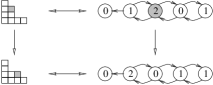
Figure 4: Coding of the Sand Pile Model with a Chip Firing Game.

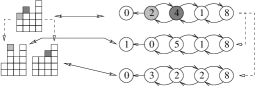
Figure 5: Coding of $L(n,\theta)$ with a Chip Firing Game when $\theta=-1$.

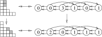
Figure 6: Coding of $CFG(n,m)$ with a Chip Firing Game when $m=2$.

Notice that the CFGs used to encode SPM, $L(n,\theta)$ and $CFG(n,m)$ contains no closed component. Therefore, we obtain the following result, previously known from [GK93], [GMP98b] and [GMP00], as a corollary of Theorem 3:

Corollary 1 ([GK93, GMP98b, GMP00])

The sets $SPM(n)$, $L(n,\theta)$ and $CFG(n,m)$ equipped with the reflexive and transitive closure of the successor relation are lattices, and these dynamical systems converge to a unique fixed point independant of the sequence of applications of the rule used. Moreover, all the paths from one configuration to another have the same length and involve the same applications of the rule.

A similar model, the Game of Cards, was introduced in [DKTR95] to study a distributed algorithm. The game is very simple: it is composed of $k$ players disposed on a ring, and each player can give a card to its right neighbour if he/she has more cards than him/her. The corresponding CFG is a ring of $k$ vertices: the $i$-th vertex has an outgoing edge to vertex $i+1$ modulus $k$ and another one to $i-1$ modulus $k$. Then, a configuration $a$ of the game is encoded by a configuration of the CFG where vertex $i$ contains as many chips as the difference between the number of cards of player $i$ and the number of cards of its right neighbour plus $1$. Notice that this codage is quite different from the previous ones, since the graph of the obtained CFG is a cycle and then it is itself a closed component. Therefore, we apply Theorem 4 and we obtain:

Corollary 2 ([GMP98a, DKTR95])

The set of extended configurations of the Game of Cards is a lattice. Moreover, each sequence of plays between two states have the same length and involve the same players.

Our last example is the Abelian Sandpile Model indroduced in physics to represent typical behaviours in granular systems and self-organised criticality [DM90, DRSV95]. The system is defined over an undirected graph with one distinguished vertex, called the sink, or the exterior. Each vertex contains a number of grains, and it can give one grain to each of its neighbours if it has more grains than its degree. This rule, called the toppling rule, is applied to every vertex except the sink. See Figure 7.

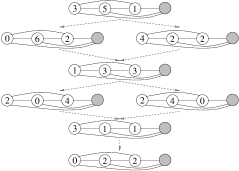
Figure 7: Behaviour of an Abelian Sandpile Model. The sink is the shaded vertex. This is equivalent to a CFG, hence the set of configurations is naturally ordered as a lattice.

The underlying graphs of the original model were $d$-dimensionnal regular finite grids with the sink representing the exterior. The model have then been extended to any graph with a sink and nice algebraic results have been developed [CR00, Mar92]. However, the fact that the configuration space of such systems is always a lattice is a new result induced by Theorem 3. Indeed, let us consider an Abelian Sandpile Model over a graph $G$ and let us construct a CFG with support $G^{\prime}$ such that the two systems are equivalent. Let $G^{\prime}$ defined by:

• If there is an undirected edge $\{i,j\}$ in $G$ then $G^{\prime}$ contains the directed edges $(i,j)$ and $(j,i)$ in $G^{\prime}$, except if either $i$ or $j$ is the sink.

• If there is an undirected edge $\{i,j\}$ in $G$ such that $j$ is the sink, then $G^{\prime}$ contains the directed edge $(i,j)$.

Now it is obvious that this CFG is equivalent to the Abelian Sandpile Model when a grain is identified with a chip. Therefore, we obtain the convergence and the fact that all the paths from one configuration to another have the same length and involve the same applications of the rule, which is proved in [DM90, DRSV95, CR00, Mar92], and one more result:

Corollary 3

Given an initial configuration, the set of reachable configuration of an Abelian Sandpile Model is a lattice.

For related models used in economics, and for which many results can be obtained from the ones presented here, we send the reader to [Heu99, Big97, Big99]. The models developed in these papers are very close to our Chip Firing Game, and the questions they study concern convergence, length of paths, and others.

5 A Note about Parallel versus Sequential CFG

The results presented until now deal with the sequential Chip Firing Game: at each step, we apply the firing rule to only one vertex among the possible ones. However, as we already noticed in the introduction, the parallel case, where we apply the firing rule to each vertex at each step, is of great interest: it represents many physical phenomenons and is a model for distributed algorithms. We will now introduce two new models which add a certain amount of parallelism to CFGs. These two generalizations seem relevant since many practical problems can be modelized this way.

The first step is the semi-parallel Chip Firing Game, denoted by $CFG(k)$, where at each step we apply the firing rule to at most $k$ vertices among the possible ones. If $k=1$, we simply obtain the sequential model. However, if $k\geq 2$, this model creates transitivity edges in the configuration space. Indeed, if for example two firings are possible from a configuration $c$, then $c$ has three successors: $c\rightarrow c^{\prime}$, $c\rightarrow c^{\prime\prime}$ and $c\rightarrow c^{\prime\prime\prime}$ where $c^{\prime}$ is obtained from $c$ by firing one of the two possible vertices, say $\nu^{\prime}$, $c^{\prime\prime}$ is obtained from $c$ by firing the other possible one, $\nu^{\prime\prime}$, and $c^{\prime\prime\prime}$ is obtained from $c$ by firing simultaneously the two vertices $\nu^{\prime}$ and $\nu^{\prime\prime}$. Notice that it is possible to fire the vertex $\nu^{\prime\prime}$ from $c^{\prime}$, and this leads to $c^{\prime\prime\prime}$. Likewise, it is possible to fire $\nu^{\prime}$ from $c^{\prime\prime}$ in order to obtain $c^{\prime\prime\prime}$. Therefore, the edge $c\rightarrow c^{\prime\prime\prime}$ is simply a transitivity edge, and one can verify that the same phenomenon appears if there are more than two vertices which can be fired, and for any $k\geq 2$. See Figure 8 for an example. This immediately implies that the semi-parallel $CFG(k)$ lead to the same final state (if any), independently of $k$.

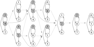
Figure 8: The configuration space of a semi-parallel CFG with $k=2$.

Now, a natural variation is the maximal semi-parallel Chip Firing Game, where we fire as much vertices as possible but no more than $k$. This model is exactly the parallel Chip Firing Game if $k$ is equal to the number of vertices of the support. On the other hand, we have the sequential Chip Firing Game when $k=1$. Moreover, it is clear that the configuration space of a maximal semi-parallel CFG is obtained from the configuration space of the corresponding semi-parallel CFG by deleting all the configurations $c_{1}$, $c_{2}$, $\dots$, $c_{l}$ such that the transitivity edge $c_{0}\rightarrow c_{l+1}$ exists, with $c_{0}\rightarrow c_{1}$ and $c_{l}\rightarrow c_{l+1}$, and then taking the configurations which are reachable from the initial one (see Figure 9). Then, it is clear that the configuration space of a maximal semi-parallel CFG is a subset of the configuration space of its corresponding sequential CFG, and that both have the same fixed point. Therefore, both sequential, semi-parallel, maximal semi-parallel and parallel CFG have the same fixed point.

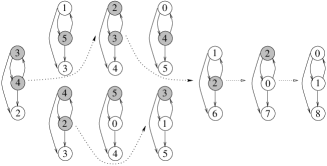
Figure 9: Construction of the configuration space of a maximal semi-parallel CFG with $k=2$. After deleting the edges for which there exists shortcuts, we simply take the configurations reachable from the initial one. Here, we finally obtain the same configuration space as in the parallel case (see Figure 1).

It seems now natural to study how the lattice properties evolves when we consider maximal semi-parallel CFGs instead of sequential ones. It should be natural to expect that the configuration space of such a game is a sub-lattice of the corresponding sequential CFG. Actually, as shown in Figure 10, this is not true since the configuration space of a maximal semi-parallel CFG is not (in this case) a sub-order of its corresponding sequential game. We can say even more from this simple example: in a maximal semi-parallel game, there exist paths of different lengths from one configuration to another. This is a very important remark, which shows that some maximal semi-parallel can not be simulated by any sequential CFG. Moreover, if each edge consists in an elementary operation in a (parallel) computer, then we can manage the calculus necessary to go from one configuration to another in an efficient way. Finally, we can see on Figure 11 that the configuration space of a maximal semi-parallel CFG is not always a lattice.

Figure 10: From left to right: the support of the considered CFG; the configuration space of the sequential CFG started in a particular configuration; the configuration space of the corresponding maximal semi-parallel CFG(k) with $k=2$. The two outlined configurations show that the order is not preserved.

Figure 11: A maximal semi-parallel CFG for which the configuration space is not a lattice when $k=2$. Notice that the support is very simple: it is nothing but the equivalent of SPM (see Section 4).

6 Perspectives

This paper shows that the structure of the configuration space of any Chip Firing Game can be viewed as a lattice. This explains the strong relation between many dynamical systems and lattices already noticed in previous papers. Moreover, the model of Chip Firing Games is very general, which leads to the possibility of proving the lattice structure of other models by coding them as special Chip Firing Games.

This also raise to another kind of questions: since the Chip Firing Games are very general, many lattices can be viewed as the configuration space of a Chip Firing Game. Lemma 2 also shows that two sequences of firings from a configuration to another one have the same length, which means that the obtained lattices are ranked. Moreover, if $a\rightarrow b$ and $a\rightarrow c$ in the configuration space of a CFG, then there exists $d$ such that $b\rightarrow d$ and $c\rightarrow d$. Therefore, there exists some lattices which are not isomorphic to any configuration space of a CFG. However, we do not know if the class of the lattices which verify these two properties corresponds exactly to the class of these lattices isomorphic to the configuration space of a CFG. If it is not the case, it should be very interesting to look for a characterization of these lattices. Likewise, the special case of distributive lattices is very interesting. Is any distributive lattice isomorphic to the configuration space of a CFG ? For example, we show in Figure 12 the CFG equivalent to the distributive lattice obtained from the empty partition by iteration of the following rule: one can add one grain to a column of a partition if one obtains this way another partition. This lattice can also be thought as the lattice of the ideals of the product of two chains, which is known to be distributive [DP90].

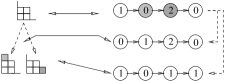
Figure 12: The coding of the partitions with addition of one grain, i.e. the ideals of the product of two chains (here, $\{{1,2,3}\}\times\{{1,2,3}\}$), with a Chip Firing Game.

Finally, an interesting open problem was pointed out by Moore and Nilsson [MN99]. They studied the special case of Abelian Sandpile Model on $d$-dimensional grids. If $d=1$, this is nothing but $SPM$. If $d\geq 3$, they proved that the problem of calculating the final state of the system started from an arbitrary configuration is P-complete. However, the case $d=2$ is still open, and it is a challenge to determine the complexity of the prediction of the final state in this case. We show here that the configuration space in each of these cases is a lattice. It should be worth to study more deeply the structure of the obtained lattice in the case $d=2$, which would lead to insight in the study of this complexity. The case $d=1$ is studied in [LMMP98]: it appears that the configuration space is strongly self-similar, which is certainly also true for $d=2$. Using this self-similarity, one may hope to obtain some interesting algorithms about the case $d=2$.

References

- [Big97] N. Biggs. Algebraic potential theory on graphs. Bull. London Math. Soc., 29:641–682, 1997.
- [Big99] N. Biggs. Chip firing and the critical group of a graph. Journal of Algebraic Combinatorics, 9:25–45, 1999.
- [BLS91] A. Bjorner, L. Lovász, and W. Shor. Chip-firing games on graphs. E.J. Combinatorics, 12:283–291, 1991.
- [Bry73] T. Brylawski. The lattice of integer partitions. Discrete Mathematics, 6:210–219, 1973.
- [BTW87] P. Bak, C. Tang, and K. Wiesenfeld. Physics Review Letters, 59:381, 1987.
- [CR00] R. Cori and D. Rossin. On the sandpile group of a graph. European Journal of Combinatorics, 21(4):447–459, 2000.
- [DKTR95] J. Desel, E. Kindler, T.Vesper, and R.Walter. A simplified proof of the self-stabilizing protocol: A game of cards. Information Processing Letters, 54:327–328, 1995.
- [DM90] D. Dhar and S.N. Majumbar. Abelian sandpile model on the bethe lattice. Journal of Physics, A 23:4333–4350, 1990.
- [DP90] B.A. Davey and H.A. Priestley. Introduction to Lattices and Orders. Cambridge university press, 1990.
- [DRSV95] D. Dhar, P. Ruelle, S. Sen, and D. Verma. Algebraic aspects of sandpile models. Journal of Physics, A 28:805–831, 1995.
- [Eri93] Kimmo Eriksson. Strongly Convergent Games and Coexter Groups. PhD thesis, Kungl Tekniska Hogskolan, Sweden, 1993.
- [GK93] E. Goles and M.A. Kiwi. Games on line graphs and sand piles. Theoretical Computer Science, 115:321–349, 1993.
- [GM97] Eric Goles and Maurice Margenstern. Universality of the chip-firing game. Theoretical Computer Science, 172:121–134, 1997.
-
[GMP98a]
E. Goles, M.Morvan, and H.D. Phan.
Lattice structure and convergence of a game of cards.
1998.
Submitted. Preprint available at
http://www.liafa.jussieu.fr/~phan/biblio.html. - [GMP98b] E. Goles, M. Morvan, and H.D. Phan. The structure of chip firing games and related models. 1998. Submitted.
- [GMP00] E. Goles, M. Morvan, and H.D. Phan. About the dynamics of some systems based on integer partitions and compositions. To appear in LNCS issue, proceedings of FPSAC’00, 2000.
-
[Heu99]
Jan van den Heuvel.
Algorithmic aspects of a chip firing game.
London School of Economics, CDAM Research Reports., 1999.
Preprint available at
http://www.cdam.lse.ac.uk/Reports/reports99.html. - [Hua93] S.-T. Huang. Leader election in uniform rings. ACM Trans. Programming Langages Systems, 15(3):563–573, 1993.
-
[LMMP98]
M. Latapy, R. Mantaci, M. Morvan, and H.D. Phan.
Structure of some sand piles model.
1998.
To appear in Theoretical Computer Science, preprint available at
http://www.liafa.jussieu.fr/~latapy/articles.html. - [Mar92] O. Marguin. Application de méthodes algébriques à l’étude algorithmique d’automates cellulaires. PhD thesis, Université Claude Bernard- Lyon 1, 1992.
-
[MN99]
C. Moore and M. Nilsson.
The computational complexity of sandpiles.
Journal of Stastistical Physics, 96:205–224, 1999.
Preprint available at
http://www.santafe.edu/~moore/.