Robustness of Quadratic Solitons with Periodic Gain

Abstract

We address the robustness of quadratic solitons with periodic non-conservative perturbations. We find the evolution equations for guiding-center solitons under conditions for second-harmonic generation in the presence of periodic multi-band loss and gain. Under proper conditions, a robust guiding-center soliton formation is revealed.

Multicolor optical soliton formation mediated by cascading of quadratic nonlinearities has been demonstrated experimentally during the last few years in a variety of geometries and frequency-mixing processes, in settings for spatial, temporal and spatio-temporal trapping of light.¹ Soliton signals exist in particular in the process of second-harmonic generation (SHG) that is addressed here, where solitons form in waveguides and in bulk crystals by the mutual trapping between the fundamental frequency and second-harmonic waves. Multidimensional soliton families exist above a threshold light intensity for all values of the phase-mismatch between the waves, and most of such solitons have been shown to be dynamically stable under propagation with the equations that model the ideal light evolution under conditions of focused and pulsed SHG. Adiabatic soliton decay and amplification in the presence of weak loss or gain, have been also studied.^2-4

In this Letter we address the robustness of quadratic solitons against strong, but periodic non-conservative perturbations. To start the program we consider soliton formation in the presence of multi-frequency losses and large, but rapidly-varying periodic gain. Our goal is to derive the corresponding guiding-center evolution equations and to expose the robustness of the existing solitons under proper conditions. We believe that the results reported bear a generic fundamental interest to the robustness of quadratic soliton formation in structures with periodic non-conservative perturbations. Moreover, they might find direct applications in reduced models of multi-color laser systems with intracavity frequency generation, including self-frequency doubling schemes, operating in the solitonic regime.^5,6

Here the focus is on solitons formed in one-dimensional structures under conditions for non-critical type I SHG, but the analysis can be extended to different physical settings. The evolution of the slowly-varying envelopes of the light waves in the presence of multi-frequency band loss and periodic gain can be described by the reduced equations⁷

$$i\frac{\partial a_{1}}{\partial\xi}-\frac{\alpha_{1}}{2}\frac{\partial^{2}a_{1}}{\partial s^{2}}+a_{1}^{*}\,a_{2}\,\exp(-i\beta\xi)=i\Gamma_{1}(\xi)a_{1},$$ (1)

$$i\frac{\partial a_{2}}{\partial\xi}-\frac{\alpha_{2}}{2}\frac{\partial^{2}a_{2}}{\partial s^{2}}+a_{1}^{2}\,\exp(i\beta\xi)=i\Gamma_{2}(\xi)a_{2},$$ (2)

where $a_{1}$ and $a_{2}$ are the normalized amplitudes of the fundamental frequency (FF) and second-harmonic (SH) waves. In the case of spatial solitons, $\alpha_{1}=-1$, and $\alpha_{2}=-k_{1}/k_{2}\simeq-0.5$, where $k_{\nu}$, with $\nu=1,2$ are the linear wave numbers at both frequencies. In the case of temporal solitons, $\alpha_{\nu}$ stand for the ratio between the group-velocity-dispersions existing at both frequencies. The transverse and longitudinal coordinates are normalized to the beam or pulse width and to the diffraction or dispersion length at the fundamental frequency, respectively. The parameter $\beta$ is the scaled phase mismatch, and $\Gamma_{\nu}(\xi)$ stand for periodic gain and loss. Let $\Gamma_{\nu}(\xi)=\Gamma_{\nu}^{(0)}+R_{\nu}(\xi)$, where $\Gamma_{\nu}^{0}$ are the average gain or loss at the FF and SH frequencies, and $R_{\nu}(\xi)$ are periodic functions, with period $L\ll 1$, and zero mean.

To derive the evolution equations of the guiding-center solitons in the presence of the periodic gain, we first use the approach originally introduced by Mollenauer, Evangelides and Haus for the case of Kerr solitons propagating in optical fibers.⁸ Let $A_{1}=a_{1}$ and $A_{2}=a_{2}\exp(-i\beta\xi)$. The explicit periodic gain can be removed from equations (1)-(2) by making the transformations $A_{\nu}(\xi,s)=U_{\nu}(\xi,s)\exp[\int_{0}^{\xi}R_{\nu}(\xi^{\prime})\mbox{d}\xi^{\prime}]$. Substitution in (1)-(2) leads to the evolution equations

$$i\frac{\partial U_{1}}{\partial\xi}-\frac{\alpha_{1}}{2}\frac{\partial^{2}U_{1}}{\partial s^{2}}-i\Gamma_{1}^{(0)}U_{1}+\epsilon_{2}(\xi)U_{1}^{*}\,U_{2}=0,$$ (3)

$$i\frac{\partial U_{2}}{\partial\xi}-\frac{\alpha_{2}}{2}\frac{\partial^{2}U_{2}}{\partial s^{2}}-i\Gamma_{2}^{(0)}U_{2}-\beta\,U_{2}+\epsilon_{3}(\xi)U_{1}^{2}=0,$$ (4)

where the resulting longitudinally-varying nonlinear coefficients write

$$\epsilon_{2}(\xi)=\exp\left[\int_{0}^{\xi}R_{2}(\xi^{\prime})\mbox{d}\xi^{\prime}\right],$$ (5)

$$\epsilon_{3}(\xi)=\exp\left[\int_{0}^{\xi}\left(2R_{1}(\xi^{\prime})-R_{2}(\xi^{\prime})\right)\mbox{d}\xi^{\prime}\right].$$ (6)

To proceed further one now assumes that the wave evolution over a period of the map is mostly dictated by the gain and loss, which are responsible for fast amplitude oscillations of the fields $A_{\nu}$, in addition to the residual effects induced by the nonlinearity. Therefore, $U_{\nu}$ vary slowly over a period of the map, so that one can average equations (3)-(4) to approximately get

$$i\frac{\partial U_{1}}{\partial\xi}-\frac{\alpha_{1}}{2}\frac{\partial^{2}U_{1}}{\partial s^{2}}-i\Gamma_{1}^{(0)}U_{1}+\eta_{2}\,U_{1}^{*}\,U_{2}\simeq 0,$$ (7)

$$i\frac{\partial U_{2}}{\partial\xi}-\frac{\alpha_{2}}{2}\frac{\partial^{2}U_{2}}{\partial s^{2}}-i\Gamma_{2}^{(0)}U_{2}-\beta\,U_{2}+\eta_{3}\,U_{1}^{2}\simeq 0,$$ (8)

where

$$\eta_{2,3}=<\epsilon_{2,3}(\xi)>=\frac{1}{L}\,\int_{0}^{L}\epsilon_{2,3}(\xi)\mbox{d}\xi,$$ (9)

are the averaged nonlinear coefficients over a period of the map. Therefore, the evolution equations for the slowly-varying averaged fields $U_{\nu,0}(\xi,s)$, defined as

$$U_{\nu,0}(\xi,s)=<\exp[\int_{0}^{\xi}R_{\nu}(\xi^{\prime})\mbox{d}\xi^{\prime}]>U_{\nu}(\xi,s),$$ (10)

write

$$i\frac{\partial U_{1,0}}{\partial\xi}-\frac{\alpha_{1}}{2}\frac{\partial^{2}U_{1,0}}{\partial s^{2}}-i\Gamma_{1}^{(0)}U_{1,0}+U_{1,0}^{*}\,U_{2,0}\simeq 0,$$ (11)

$$i\frac{\partial U_{2,0}}{\partial\xi}-\frac{\alpha_{2}}{2}\frac{\partial^{2}U_{2,0}}{\partial s^{2}}-i\Gamma_{2}^{(0)}U_{2,0}-\beta\,U_{2,0}+\eta\,U_{1,0}^{2}\simeq 0,$$ (12)

where $\eta=\eta_{2}\eta_{3}/\eta_{1}^{2}$, with $\eta_{1}=<\epsilon_{1}(\xi)>$, and

$$\epsilon_{1}(\xi)=\exp\left[\int_{0}^{\xi}R_{1}(\xi^{\prime})\mbox{d}\xi^{\prime}\right].$$ (13)

One thus concludes that under the conditions where the approximations used to derive (11)-(12) hold, the guiding-center solitons are given by those existing without gain and loss when $\Gamma_{\nu}^{(0)}=0$,⁹ or otherwise with compensated gain and loss,¹⁰ but with properly renormalized amplitudes. To expose the value and dependencies of the renormalization coefficient $\eta$, consider the illustrative map $R_{\nu}(\xi)=G_{\nu}\,H(\xi)$, where $H(\xi)$ is the Heaviside function

$$H(\xi)=\left\{\begin{array}[]{ccl}-1,&&nL<\xi<(n+1/2)L,\\ 1,&&(n+1/2)L<\xi<(n+1)L.\end{array}\right.$$ (14)

Substitution in the above expressions and performing all the averages yields

$$\eta=\frac{F[G_{2}L/2]F[(2G_{1}-G_{2})L/2]}{F^{2}[G_{1}L/2]},$$ (15)

where

$$F[\mu]=\frac{1-\exp(-\mu)}{\mu}.$$ (16)

Of particular interest are the weak maps with $\mu\ll 1$, corresponding to $G_{\nu}L\ll 1$. In such cases, one might expand (15) in powers of the corresponding parameters to get, at order $L^{2}$

$$\eta\simeq 1\,+\,\frac{(G_{1}-G_{2})^{2}L^{2}}{48}.$$ (17)

Note that when $G_{1}=G_{2}$, equation (15) gives $\eta=1$, regardless the value of the map period $L$. However, this does not mean that the guiding-center evolution is given by (11)-(12) with $\eta=1$ at all orders of $L$, because the derivation of (11)-(12), hence the governing equations themselves, are only intended to hold when $L\ll 1$. To elucidate the applicability limits of (11)-(12), it is worth deriving the guiding-center evolution equations using more mathematically systematic approaches.^11,12 Next we outline the outcome of the asymptotic expansion method developed by Kivshar and co-workers for similar problems but for Kerr solitons.¹² Such approach has been recently employed to obtain guiding-center evolution equations of light signals propagating in quasi-phase-matched quadratic structures.¹³

Assuming perfect periodicity of the functions $R_{\nu}(\xi)$ as above, one can express the periodic gain and all fields as Fourier series of the form

$$R_{\nu}(\xi)=\sum_{n\neq 0}d_{\nu,n}\exp(in\lambda\xi),$$ (18)

$$A_{\nu}(\xi,s)=\sum_{n}U_{\nu,n}(\xi,s)\exp(in\lambda\xi),$$ (19)

where $\lambda=2\pi/L$ and the Foruier coefficients $U_{\nu,n}(\xi,s)$ vary much slower than the corresponding carrier $\exp(in\lambda\xi)$. For the map (14) considered here one has

$$d_{\nu,2n}=0,\qquad d_{\nu,(2n+1)}=\frac{2G_{\nu}}{i\pi(2n+1)}.$$ (20)

Assuming the amplification maps to vary rapidly over a diffraction/dispersion lenght, i.e. $L\ll 1$, so that the spatial frequency $\lambda$ is large enough, one can expand the harmonic amplitudes $U_{\nu,n\neq 0}$, as power series of $1/\lambda$. Namely,

$$U_{\nu,n\neq 0}=\sum_{m>0}\frac{F_{\nu,n}^{(m)}}{\lambda^{m}}.$$ (21)

Substitution in the governing equations and matching leading-order contributions leads to

$$F_{\nu,n}^{(1)}=-i\,\frac{d_{\nu,n}}{n}\,U_{\nu,0}.$$ (22)

The guiding-center evolution is obtained by solving recursively for the higher-order contributions $F_{\nu,n}^{(m>1)}$ and substituting the corresponding expressions in the evolution equations for the average fields $U_{\nu,0}$. At order $1/\lambda^{2}$, one exactly finds (11)-(12), with (17).

Equations (11), (12) and (17) are the central result of this paper. First, they reveal that when $G_{1}=G_{2}$, at order $L^{2}$ the guiding-center evolution equations are identical to those without the periodic gain, regardless the value of the amplitudes $G_{\nu}$. This is a remarkable result, that emphasizes the robustness of quadratic solitons with the type of perturbations considered. Second, the typical values of the gain coefficient that is obtained in Erbium-doped lithium niobate or potassium titanyl phosphate around the third telecommunication window centered at 1.55 $\mu$m fall in the range 0-2 dB/cm.^5,14 In the case of spatial solitons, this yields values of the normalized gain coefficient of the order of $G_{\nu}\sim 10^{-1}$.³ With such values and letting $L\sim 10^{-1}$, one always obtains negligible corrections of the order of $[\eta-1]\sim 10^{-5}$.

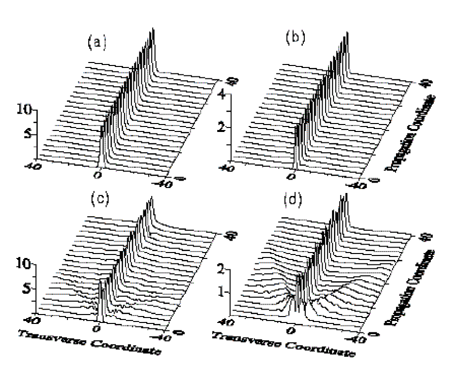
FIG. 1.: Typical evolution of guiding-center quadratic solitons in structures with rapidly-varying periodic gain. In (a)-(b): The input is a renormalized stationary soliton solution. In (c)-(d): The input contains only fundamental frequency light with a Gaussian shape. (a), (c) : Evolution of the FF; (b), (d): Evolution of the SH. Conditions: $\beta=3$, $\tilde{I}=30$, $G_{1}=20$, $G_{2}=0$, $L=0.2$.

To confirm that under proper conditions (11)-(12) hold, we solved (1)-(2) numerically for different input conditions and maps. Figure 1 shows typical examples of the outcome, when $\Gamma_{\nu}^{(0)}=0$. The plots correspond to the phase-mismatch $\beta=3$, but analogous results were obtained for other values. To emphasize that guiding-center solitons form with gigantic values of the gain-loss amplitude, provided that the period of the map is small enough so that the guiding-center approach is justified, we display results for a map with $G_{1}=20$, $G_{2}=0$ and $L=0.2$. Figures 1(a)-(b) show the propagation of a guiding-center soliton excited by the input $A_{\nu}(0)=\tilde{A}_{\nu}(0)/\rho_{\nu}$, where $\tilde{A}_{\nu}(0)$ are the corresponding stationary solitons existing without gain and loss with energy flow $\tilde{I}=\tilde{I}_{1}+\tilde{I}_{2}=\int(|\tilde{A}_{1}|^{2}+|\tilde{A}_{2}|^{2})\mbox{d}s=30$,⁹ while $\rho_{1}=(\eta_{2}\eta_{3})^{1/2}$, and $\rho_{2}=\eta_{2}$, are the renormalization factors dictated by (7)-(8). For the map considered one has $\rho_{1}\sim 0.5$, so that in the renormalized input the FF energy is enhanced by a factor of four. Figures 1(c)-(d) show the excitation of a guiding-center soliton in the same map but with only FF input light carrying the same energy flow as above in the Gaussian shape $A_{1}(0)=(2/\pi)^{1/4}\,I_{1}^{1/2}\exp(-s^{2})$. Here $I_{1}=\tilde{I}_{1}/\rho_{1}^{2}$.

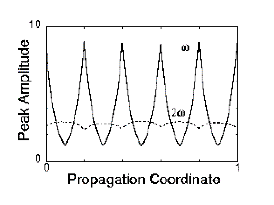
FIG. 2.: Detail of the evolution of the peak amplitudes of the signals displayed in Figs. 1(a)-(b), over the first five periods of the map.

Figure 2 shows the detailed evolution of the field amplitudes in the case shown in Figs. 1(a)-(b). Because of the large excursions of the amplitudes, the actual evolution differs slightly from that predicted by equations (11)-(12). Such departures are responsible, e.g., of the small resonance peaks appearing in the Fourier spectra of the FF and SH evolving signals, as shown in Figure 3.

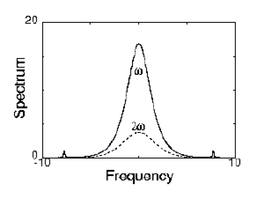
FIG. 3.: Fourier spectra of the FF and SH signals displayed in Figs. 1(a)-(b), at $\xi=40$.

When $\Gamma_{\nu}^{(0)}\neq 0$, but the net loss at one frequency is compensated for by the presence of a net gain at the other frequency band, the system (11)-(12) allows stationary soliton solutions,¹⁰ which are chirped. However, an interesting result revealed by the guiding-center evolution equations (11)-(12) is that, in the absence of a net gain or loss (i.e., $\Gamma_{\nu}^{(0)}=0$), on average the guiding-center quadratic solitons are chirpless. Accordingly, in contrast to what is found with solitons in other periodic systems, e.g., with dispersion-managed solitons propagating in optical fibers,¹⁵ one concludes that with chirpless input conditions the guiding-center quadratic solitons with periodic gain are best excited when the first domain has the whole nominal length. The outcome of our numerical simulations confirms that such is indeed the case, as shown in Figure 4. The plot shows the evolution over a period of the map of the quantities

$$C_{\nu}(\xi)=\frac{i}{4}\,\frac{\int s(A_{\nu}A_{\nu,s}^{*}-A_{\nu}^{*}A_{\nu,s})\,\mbox{d}s}{\int s^{2}|A_{\nu}|^{2}\,\mbox{d}s},$$ (23)

where $A_{\nu,s}$ stands for $\partial A_{\nu}/\partial s$. The evolution displayed corresponds to a guiding-center soliton similar to that shown in Figs. 1(a)-(b), but for $G_{1}=G_{2}=10$.

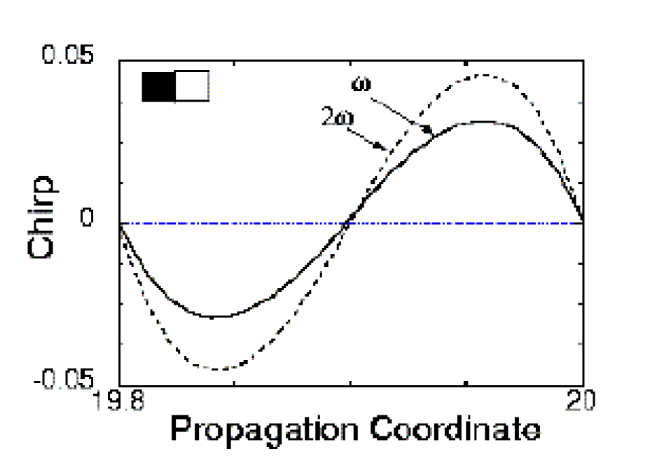
FIG. 4.: Typical evolution of the integral chirp of the guiding-center solitons over a period of the map. The plot shows the evolution from $\xi=19.8$ to $\xi=20$. Conditions: $\beta=3$, $\tilde{I}=30$, $G_{1}=10$, $G_{2}=10$, $L=0.2$. The input is the corresponding renormalized stationary soliton solution.

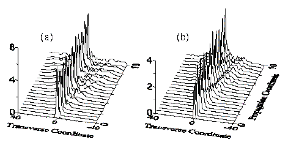
FIG. 5.: Unstable evolution when the guiding-center approach fails. The input is a renormalized stationary soliton solution. Same conditions as in Figs. 1(a)-(b), except that here $G_{1}=2$ and $L=1$. (a): Evolution of the FF; (b): Evolution of the SH.

Analogous results than those shown above were obtained for a variety of values of the phase-mismatch $\beta$, the input energy flow $I$, the signal shape, and the map amplitude. Naturally, this is so provided that the input conditions, the gain amplitude, and the period $L$ make a guiding-center approach justified.^11-12 Otherwise, e.g., when $L$, $G_{\nu}$ or the input $I$ are too large, the guiding-center evolution fails, yielding a totally new scenario. In particular, under such conditions resonance phenomena that make the wave propagation unstable can occur. Figure 5 shows a typical example. The plot shows the unstable evolution of the renormalized solution with $\tilde{I}=30$ in a map with $G_{1}=2$, with $L=1$.

In conclusion, the evolution equations for guiding-center quadratic solitons propagating in structures with multi-frequency losses and rapidly-varying periodic gain have been presented. Under proper conditions, robust multicolor quadratic soliton formation has been revealed. Results might find applications to reduced models of multicolor laser systems with intracavity frequency generation, including self-frequency doubling schemes, operating in the solitonic regime. Extension of the analysis to general maps that include the details of the laser structures, including the pump light-matter interaction,^5,14 is worth investigating.

This work was supported by the Generalitat de Catalunya. Ole Bang acknowledges support from the Danish Technical Research Council through Talent Grant No. 9800400.

REFERENCES

- [1] G. I. Stegeman, D. J. Hagan, and L. Torner, Opt. Quantum Electron., 28, 1691 (1996); M. Segev and G. I. Stegeman, Phys. Today 51, 42 (1998).
- [2] K. Hayata and M. Koshiba, J. Opt. Soc. Am. B 12, 2288 (1995); L. Torner, D. Mihalache, D. Mazilu, and N. N. Akhmediev, Opt. Lett. 20, 2183 (1995); B. A. Malomed, D. Anderson, A. Berntson, M. Florjancyk, and M. Lisak, Pure Appl. Opt. 5, 941 (1996).
- [3] L. Torner, Opt. Commun. 154, 59 (1998).
- [4] S. Darmanyan, A. Kobyakov, and F. Lederer, Opt. Lett. 24, 1517 (1999).
- [5] T. Y. Fan, A. Cordova-Plaza, M. J. F. Digonnet, R. L. Byer, and H. J. Shaw, J. Opt. Soc. Am. B 3, 140 (1986); J. Capmany, E. Montoya, V. Berm dez, D. Callejo, E. Di guez, L. E. Baus , Appl. Phys. Lett. 76, 1374 (2000); A. V. Kir’yanov, I. V. Mel’nikov, K. Wagner, Appl. Phys. Lett. 76, 2829 (2000).
- [6] P.-S. Jin, W. E. Torruellas, M. Haelterman, S. Trillo, U. Peschel, and F. Lederer, Opt. Lett. 24, 400 (1999).
- [7] C. R. Menyuk, R. Schiek and L. Torner, J. Opt. Soc. Am. B 11, 2434 (1994).
- [8] L. F. Mollenauer, S. G. Evangelides, and H. A. Haus, J. Lightwave Technol. LT-9, 194 (1991).
- [9] A. V. Buryak, Y. S. Kivshar, Phys. Lett. A 197, 407 (1995); L. Torner, Opt. Comm. 114, 136 (1995).
- [10] L.-C. Crasovan, B. Malomed, D. Mihalache, and F. Lederer, Phys. Rev. E 59, 7173 (1999); L. Torner, J. D rring, and J. P. Torres, IEEE J. Quantum Electron. QE-34, 1344 (1999).
- [11] A. Hasegawa and Y. Kodama, Solitons in Optical Communications (Clarendon, Oxford, 1995).
- [12] Y. S. Kivshar, K. Spatschek, S. Turitsyn, and M. L. Quiroga-Teixeiro, Pure Appl. Opt. 4, 281 (1995).
- [13] C. B. Clausen, O. Bang, and Y. S. Kivshar, Phys. Rev. Lett. 78, 4749 (1997); O. Bang, C. B. Clausen, P. L. Christiansen, and L. Torner, Opt. Lett. 24, 1413 (1999).
- [14] C. Becker, T. Oesselke, J. Pandavenes, R. Ricken, K. Rochhausen, G. Schreiber, W. Sohler, H. Suche, R. Wessel, S. Balsamo, I. Montrosset, D. Sciancalepore, IEEE J. Selected Topics Quantum Electron. 6, 101 (2000); V. Berm dez, J. Capmany, J. Garc a-Sol , E. Di guez, Appl. Phys. Lett. 73, 593 (1998).
- [15] See, e.g., S. K. Turitsyn, V. K. Mezentsev, and E. G. Shapiro, Opt. Fiber Technol. 4, 384 (1998).