Scarring Effects on Tunneling in Chaotic Double-Well Potentials

Abstract

The connection between scarring and tunneling in chaotic double-well potentials is studied in detail through the distribution of level splittings. The mean level splitting is found to have oscillations as a function of energy, as expected if scarring plays a role in determining the size of the splittings, and the spacing between peaks is observed to be periodic of period $2\pi\hbar$ in action. Moreover, the size of the oscillations is directly correlated with the strength of scarring. These results are interpreted within the theoretical framework of Creagh and Whelan. The semiclassical limit and finite-$\hbar$ effects are discussed, and connections are made with reaction rates and resonance widths in metastable wells.

I Introduction

Many chemical reactions must proceed through a potential barrier before the final dissociation of the products of the reaction can take place. Thus, the reaction rate is governed by tunneling [2]. Radioactive decay of nuclei also involves crossing a potential barrier, dictated by a combination of short-ranged strong binding forces and a longer-ranged Coulomb repulsion [3]. A typical experimental situation is the absorption of a slow neutron; the resulting metastable nucleus decays predominantly by tunneling through a saddle point, and the distribution of resonance widths is well described by random matrix theory [4]. Another important example of quantum tunneling is the conductance of mesoscopic devices [5]. In more than one dimension, when the classical dynamics can be chaotic, quantum chaos plays a role. For instance, in the tunneling diode junction, in which electrons are driven by an applied electric field but must tunnel through potential barriers at either end of the device, the dynamics, in the presence of a magnetic field, is chaotic and scarring of a short periodic orbit is known to dominate the conduction [6]. In this paper we study chaotic tunneling in a simple model potential, and establish the connection to scar theory, both qualitatively and quantitatively. We prefer to study tunneling by calculating splittings in a double-well potential rather than resonance widths in a metastable well, because the former is an easier computational task, as we will see later in Sec. II. The relation between splittings in a double-well potential and resonance widths in a metastable well will be discussed immediately below, where we will observe that the two quantities are related by known overall normalization factors.

The double-well potential we will work with, in two dimensions, has the very simple form

$$V(x,y)=x^{4}-x_{0}^{2}x^{2}+ay^{2}+\lambda x^{2}y^{2}+\sum_{i}b_{i}e^{-((x-x_{i})^{2}+(y-y_{i})^{2})/\sigma_{i}^{2}}\,.$$ (1)

The parameters $x_{0}$, $a$, $\lambda$, $b_{i}$, $x_{i}$, $y_{i}$ and $\sigma_{i}$ will be specified below. For $x_{0}^{2}>0$, a barrier along the $y$-axis separates the potential at low energies ($E<0$) into two wells. The $\lambda x^{2}y^{2}$ term ensures that the potential is not separable, while the Gaussian perturbations, the parameters of which may be changed at will, allow us to generate an ensemble of statistically independent eigenstates near any given energy. If the positions and heights of the Gaussians are chosen suitably, the potential has reflection symmetries in the $x$ and $y$ directions. The symmetry under reflection in $y$ means that there will always be a short periodic orbit on the $x$-axis, in each of the two wells.

The principal result of this paper is that the size of the level splittings in the two-dimensional double well, the classical dynamics of which is chaotic, is directly correlated with the scarring of eigenfunctions along the $x$-axis, which we believe to be the primary channel for tunneling. The evidence for this is that (1) the distribution of splittings, once the average exponential trend in energy is scaled out, displays oscillations as a function of energy of the sort expected by scar theory. In particular, the action distance between successive peaks is precisely $h$. However, the dependence of the mean splitting on action is not well reproduced quantitatively by linear scar theory, because non-linear effects appear to be important. (2) The rescaled splittings are correlated with the overlap of the eigenstate with a Gaussian test state lying on the periodic orbit on the $x$-axis, a measure of scarring. (3) The correlation of the splittings with the overlaps is further supported by the fact that the distribution of overlaps has the same energy-dependent oscillations as the distribution of splittings.

According to one-dimensional WKB theory, the splitting $\Delta E=E_{\rm anti-symm}-E_{\rm symm}$ in a symmetric double well is given in the semiclassical limit by

$$\Delta E=\left({{\hbar\omega}\over\pi}\right)e^{-S/\hbar}\,,$$ (2)

while the resonance width $\Gamma$ for the state at the same energy in a metastable well is

$$\Gamma=\left({{\hbar\omega}\over{4\pi}}\right)e^{-2S/\hbar}\,.$$ (3)

Here $\omega$ is the frequency of the classical periodic motion at energy $E_{\rm symm}$ and the imaginary action for going under the barrier is

$$S=\int_{-x_{\rm tp}}^{x_{\rm tp}}\,dx\,\sqrt{V(x)-E}\,,$$ (4)

$x_{\rm tp}>0$ being the position of the classical turning point at energy $E_{\rm symm}$ [7]. In order for the semiclassical theory to apply, $E_{\rm symm}$ must be sufficiently far below the barrier that $S/\hbar\gg 1$. Note the factor of two in the exponent in Eq. (3).

These one-dimensional formulae may be generalized to the two-dimensional (or higher-dimensional) potential well as follows. We expect tunneling to be dominated by paths that cross the barrier close to the $x$-axis, which has the smallest action integral $S$. The splitting $\Delta E$ will then be proportional to the exponential factor $e^{-S/\hbar}$.

The correct generalization of the frequency of attempts to cross the barrier, $\omega$, to two or more dimensions, is the frequency with which one returns to a Planck-sized cell in phase space that lies on the horizontal periodic orbit. This horizontal periodic orbit is the real continuation of the least-action path across the barrier. The time for returning to such a cell (or to any other cell in an ergodic well) is the Heisenberg time $T_{H}=h/\Delta(E)$, where $\Delta(E)$ is the mean level spacing near energy $E$ (i.e., the spacing between doublets in the double-well system). Then the frequency of attempts to cross the barrier is just proportional to the mean level spacing $\Delta(E)$. Thus, we expect on general grounds that the splitting $\Delta E$ is given in order of magnitude by $\Delta E\sim\Delta(E)e^{-S(E)/\hbar}$, which gives us the trend of the splittings as a function of energy. This expression for the mean splitting will be confirmed by the exact semiclassical theory to be discussed below.

For any given state, we should expect that its splitting will be large or small compared with the mean value at that energy according to whether its amplitude is large or small on the horizontal periodic orbit which leads to optimal tunneling. For simplicity we can study the wave function amplitude near the turning point of the horizontal periodic orbit. The value of the wave function at the turning point in the two-dimensional chaotic system is (ignoring scar-related effects which are the main focus of this paper) given approximately by a Gaussian-distributed random variable, as random matrix theory would predict. Thus, $|\psi(x_{\rm tp})|^{2}$ has, according to random matrix theory, a Porter–Thomas distribution for all energies far enough below the barrier (near zero energy the horizontal periodic orbit becomes stable and the distribution of splittings rolls over to one having many more large and small splittings, corresponding to wave functions that live near or avoid this stable orbit). However, what is relevant to tunneling in $d$ dimensions is not just the value of the wave function exactly at the turning point but rather its behavior in a whole $\hbar^{d-1}-$sized region surrounding the periodic orbit. We shall see below that the right quantity to consider is the inner product of the wave function with a Gaussian centered on the periodic orbit (at the turning point or at some other location). This has as well a Porter–Thomas distribution, within the random matrix theory approximation. Scar-related effects and finite-$\hbar$ effects on the distribution of splittings will be discussed below.

The viewpoint summarized above is in agreement with the theoretical work of Creagh and Whelan [8]. First, they find that the mean splitting $\langle\Delta E\rangle$ at a given energy is given by the product of an exponential factor $e^{-S/\hbar}$, a factor proportional to the mean spacing between doublets, as described above, and a third factor that carries information about the monodromy matrix of the (imaginary time) tunneling orbit. Then they show that, for chaotic and symmetric double wells, the splitting for a particular eigenvalue, relative to the mean splitting, may be written in the semiclassical limit as a matrix element of the wave function $\psi$ near the real continuation ${\cal R}$ of the complex trajectory that passes through the barrier with minimum (imaginary) action. This imaginary-time trajectory and its real-time continuation may be thought of as the optimal route for tunneling. The matrix element $\Delta E\sim\langle\psi|{\cal T}|\psi\rangle$ involves integration over a Poincaré surface transverse to the real continuation ${\cal R}$. The kernel ${\cal T}$ is a semiclassical Green’s function which, in the approximation that the dominant contribution to the tunneling matrix element comes from the neighborhood of ${\cal R}$, becomes a Gaussian centered on the intersection of ${\cal R}$ with the Poincaré section. The width of the Gaussian is of $O(\hbar^{1/2})$ in both directions (e.g. $y$ and $p_{y}$) tangent to the surface of section. [The results may of course be easily generalized to dimensions $d>2$, where the resulting Gaussian has width of $O(\hbar^{1/2})$ in all $2d-2$ directions along the surface of section.]

In the case that the real continuation ${\cal R}$ happens to lie on a short periodic orbit, which will always be true when a reflection symmetry across the $x$-axis is present, this matrix element may be regarded as a measure of scarring on the periodic orbit. The Creagh–Whelan theory predicts, therefore, that strong scarring should be correlated with large splittings, confirming the intuitive expectation that high tunneling rates should occur for those wave functions that have large amplitude along the path with optimal tunneling. Neither in Ref. [8] nor in Ref. [9], however, do the authors demonstrate the connection between scarring and splittings on a state-by-state basis. In the latter work, they confirm their formula for the tunneling matrix element by deriving from it an analytical prediction for the statistical distribution of splittings. This prediction is in agreement with numerical calculations for potentials in which the real continuation of the optimal tunneling orbit is not a periodic orbit; when it is, the random-matrix assumption in their derivation breaks down due to scarring on this periodic orbit. Thus, the present paper, while confirming the predictions of Creagh and Whelan, goes beyond their results by establishing conclusively the link between scarring and tunneling and by showing, with better statistics, that the distribution of scaled splittings indeed becomes approximately Porter–Thomas, but only after scarring effects have been taken into account.

II Method

The wave functions and splittings were calculated numerically using the discrete variable representation [10]. The matrix elements of the position operators $X$ and $Y$ and of the kinetic energy operators $K_{x}$ and $K_{y}$ were first evaluated analytically using standard identities, in a basis of up to the first 300 Gauss-Hermite functions in each dimension. Then, in order to take advantage of the two reflection symmetries in $x$ and $y$, the two operators $X^{2}$ and $Y^{2}$ were diagonalized. The reason for using $X^{2}$ and $Y^{2}$ instead of the usual choice of $X$ and $Y$ is that $X^{2}$, $K_{x}$, $Y^{2}$ and $K_{y}$ are all block-diagonal, connecting only basis elements within one of the four symmetry classes (even–even, even–odd, odd–even and odd–odd). Since we are interested only in even–even potentials of the form $V(X,Y)=\sum_{i}f_{i}(X^{2})g_{i}(Y^{2})$ we can just as well compute $V$ at the eigenvalues of $X^{2}$ and $Y^{2}$ as at those of $X$ and $Y$, but using the basis obtained by diagonalizing $X^{2}$ and $Y^{2}$ ensures that the final Hamiltonian $H=K_{x}+K_{y}+V$ will be itself also block diagonal. The four symmetry classes may therefore be analyzed separately. In the basis chosen the potential $V$ is of course diagonal, while, in two or more dimensions, the kinetic energy matrix will be sparse. More precisely, if $N$ is the dimension of one of the blocks in the Hamiltonian matrix, the total number of non-zero matrix entries scales as $N^{1+1/d}$, or $N^{3/2}$ in the two-dimensional system. Since we require large values of $N$ in order to observe semiclassical behavior, a sparse matrix routine is the method of choice for diagonalizing $H$. The accuracy of the computed eigenvalues was tested for convergence under increase of $N$, and for the parameters given below we found convergence to $\pm 10^{-12}$ for $N\approx 3500$, corresponding to about 200 Gauss-Hermite functions in the $x$ direction and about 100 in the $y$ direction.

The amount of phase space covered by the region $E<0$, and thus the number of states under the barrier and the computation time, increases very rapidly with $x_{0}$. If all other parameters in the Hamiltonian are kept fixed, the number of states grows as $x_{0}^{6}$, and so the largest value of $x_{0}$ we can easily attain is about $x_{0}=6$, for $a=1$ and $\lambda=10$. At these parameter values, each well has a depth of $x_{0}^{4}/4=324$ and about 100 bound states, where $\hbar$ is taken to be unity here and in the following. The typical level spacing near the top of the well is $\sim 1$, and the splittings range from $<1$ near the top of the well to $<10^{-6}$ near $E=-50$; below this energy many of the splittings become too small ($<10^{-12}$) to be resolved numerically. Therefore we take $E=-50$ to be the lower cutoff for the energies to be analyzed in Sec. III.

III Results

The potential given by Eq. (1), apart from the Gaussian perturbation, is mostly integrable for all energies except those near the top of the barrier. When the Gaussian perturbations are introduced, the classical mechanics becomes more chaotic, but if these perturbations are too small it is still possible that they would not be seen by the quantum mechanics, which would remain effectively integrable. Thus, in order to render the quantum mechanics at energies corresponding to the bound states chaotic as well, it is necessary to introduce a Gaussian perturbation that is at least as large as the wavelength in question, and whose height is comparable in magnitude to the depth of the potential well. The simplest choice is to place large Gaussian perturbations above the minima of the potential well at $(\pm x_{0}/\sqrt{2},0)$, which will be seen by every bound trajectory as it crosses the center of the well and which thus effectively make the dynamics chaotic at energies down to the lowest considered ($E=-50$). This was checked classically by examining the Poincaré surfaces of section and may also be seen to be true quantum-mechanically in Fig. 1, where typical eigenfunctions are shown. Here, we have chosen the parameters of the double-well potential to be $x_{0}=6$, $a=1$ and $\lambda=10$, and for the central Gaussian perturbation we use a height $b=150$ (to be compared with a well depth of $V(\pm x_{0}/\sqrt{2},0)=-324$) and a width $\sigma=0.5$.

We generate an ensemble of 625 systems by placing four further Gaussians (and their reflections in $x$ and $y$) at $x=\pm 2,\pm 3,\pm 4,\pm 5$ and $y=\pm 1$, with heights $b_{i}=20n_{i}$, $n_{1},\ldots,n_{4}=1,\ldots,5$, and with equal widths $\sigma_{i}=0.5$ as above. A contour plot of the potential for a typical member of the ensemble is given in Fig. 2; note the symmetrical distortion of the contours due to the perturbation.

We proceed to analyze statistically the splittings between states in the even–even and even–odd sectors. The results, for the parameters described, are given in Figs. 3 and 4. As expected, the size of the splittings falls off exponentially with decreasing energy in Fig. 3, as the barrier becomes wider and tunneling is suppressed. The trend is approximately linear on a semi-log plot, over six decades as $E$ varies from 0 to $-50$. In Fig. 4 we rescale the splittings as a function of energy by $s\rightarrow s/e^{-S(E)}$. We find very pronounced oscillations in the distribution of splittings as a function of energy. As discussed in Sec. I, we expect theoretically that the rescaled splitting should be proportional to the overlap in a Poincaré section of the eigenfunction with a Gaussian on the horizontal periodic orbit. If the Gaussian may be assumed to have area exactly $h$ in the Poincaré section, such overlaps are described by scar theory [11, 12, 13]. We expect the results to be qualitatively the same even if the Gaussian in the Poincaré section given by the theory of Creagh and Whelan is not a minimum-uncertainty state, as long as it is not too large compared to $h$ (in the latter limit, scar effects must go to zero in accord with the Schnirelman ergodicity theorem [14]). In fact, in the data presented below the area of the Creagh–Whelan Gaussian ranged from $1.5h$ to $4h$. The prediction of scar theory is that, at a given energy, the distribution of splittings should be Porter–Thomas, and that the mean wave function intensity and therefore the mean splitting should oscillate as energy is varied by an amount that depends on the Lyapunov exponent and the monodromy matrix of the unstable periodic orbit. An important confirmation of the scarring picture is obtained when we plot, in Fig. 5, the rescaled splittings versus the action (divided by $2\pi$) of the horizontal periodic orbit at the energy eigenvalue. We find that the oscillations are periodic in action with period $2\pi$, which indicates that the EBK quantization condition for scarring holds. The EBK quantization condition for the action reads $A=2\pi(n+1/2+n_{c}/4)$ where $n$ is an integer and $n_{c}$ is the number of conjugate points in one period of the orbit ($n_{c}=3$ in the case of the horizontal orbit in our system).

A direct correlation between splittings and scarring is found by plotting, in Fig. 6, the rescaled splitting of each eigenvalue versus the overlap of the corresponding eigenfunction with a Gaussian test state lying on the horizontal periodic orbit, a measure of the degree with which this eigenfunction is scarred. The two quantities are correlated, with a slope of 2 on a log-log scale. The correlation coefficient of the logarithms is 0.78; it may be that the degree of correlation would be improved if the Gaussian were chosen to be properly aligned with respect to the monodromy matrix of the optimal tunneling path. The observed correlation nevertheless confirms that there is a direct connection, on a state-by-state basis, between scarring and tunneling, as predicted by the theory of Creagh and Whelan [8]. As a check on our results, we show in Fig. 7 that the overlaps display the same energy-dependent oscillations as do the splittings, as they must if the phenomenon of scarring underlies the behavior of both.

The connection between scarring and tunneling can be tested quantitatively in two ways. First, scar theory in the semiclassical limit predicts that the short-time (smooth) envelope describing the oscillations in the mean rescaled splitting versus action is given by the Fourier transform of the autocorrelation function $A(m)=\langle\phi|\phi(m)\rangle$, where $\phi$ is a Gaussian wave packet (living in the Poincaré section) centered on the horizontal periodic orbit and $\phi(m)$ is its iterate after $m$ bounces. The Gaussian $\phi$ is chosen to have the same orientation and aspect ratio in the $(y,p_{y})$-plane as the Gaussian called for by the Creagh–Whelan theory, but linearly rescaled so as to have area $h$ as needed for scar theory. Linearizing the dynamics around the horizontal periodic orbit we find, when the Gaussian wave packet is optimally aligned along the stable and unstable manifolds of the periodic orbit,

$$A(m)={1\over{\sqrt{\cosh\lambda m}}}\,,$$ (5)

where $\lambda$ is the Lyapunov exponent of the periodic orbit. In the special case of orthogonal stable and unstable manifolds, a circular Gaussian will be one example of an optimally aligned wave packet. If the Gaussian is not optimally aligned, this formula may be generalized as follows:

$$A(m)=2\sqrt{{{\det(M)}\over{\det(M+(J^{-m})^{T}MJ^{-m})}}}\,,$$ (6)

where $M$ describes a Gaussian of the form $({\rm const})\exp(-x^{T}Mx)$ with $x=(y,p_{y})^{T}$ representing the coordinates in the surface of section, and $J$ is the Jacobian of the Poincaré mapping evaluated at the periodic orbit (${\rm Tr}\;J=2\cosh\lambda$). The matrix $M$ is computed as specified in the Creagh–Whelan theory from the monodromy matrix of the complex orbit that begins at the Poincaré section on the right, goes through the barrier, and ends at the Poincaré section in the left well [8]. Here, the Lyapunov exponent $\lambda$ and Jacobian $J$ vary with energy over the range $-50<E<-9$. At higher energies, the trajectory spends less time near the Gaussian at the center of the well, and thus experiences less deflection, leading to greater stability, eventually becoming stable for $E>-9$. The short-time envelope obtained as the Fourier transform of $A(m)$ in either Eq. (5) or Eq. (6) may be compared with the mean rescaled splitting plotted versus action. As shown in Fig. 8, with either form of the autocorrelation function we do find peaks in the predicted envelope of splittings at the right values of action for energies $E<-9$ (for energies $E>-9$ the horizontal periodic orbit becomes stable, so the scar theory does not apply and no prediction about the distribution of splittings can be made), but the heights of the maxima and minima between the peaks are not well reproduced. The contrast predicted by Eq. (6) is closer to the numerical data than that predicted by Eq. (5). The quantitative failure of semiclassical scar theory is attributable to the fact that, for our parameter values, the linearizable region around the horizontal periodic orbit is not large compared to $h$. In fact, the size of the linearizable region is only about 0.15$h$ for the energies considered. Its size, however, is approximately independent of energy for $-50<E<0$, and this may explain the weak dependence of the peak height on energy observed in the numerical data. Nevertheless, we see that not only is scarring associated with larger splittings in the coarse sense of Fig. 6 but also the enhancement factor in the distribution of splittings, as a function of energy or of action, does oscillate with energy or action in agreement with the analytical prediction of scar theory; only the precise magnitude of these oscillations remains unexplained within the present linear theory.

A second quantitative test of scar theory in relation to tunneling is to examine the change in the distribution of splittings upon change in the Lyapunov exponent. The horizontal periodic orbit can easily be made more stable by keeping the height of the main Gaussian bump fixed at 150 while increasing its width. An ensemble of eigenstates and associated splittings was computed, just as above, for a larger value of the bump width, namely $0.63$ instead of $0.50$. The expectation from scar theory would be for the distribution of splittings to have many more smaller and larger splittings at the resulting smaller Lyapunov exponent. At $\sigma=0.5$, the horizontal periodic orbit is stable down to $E=-9.1$; the Lyapunov exponent then increases from zero with decreasing energy to a value of $\lambda=2.0$ at $E=-50$. For $\sigma=0.63$ it is stable down to $E=-49.8$ and attains only a value of $\lambda=0.11$ at $E=-50$. The numerical data, however, show no marked difference between the two computations at $\sigma=0.5$ and $\sigma=0.63$; see Fig. 9. The lack of any difference between the distributions of splittings despite the difference in stability is an indication that we are not far enough into the semiclassical limit (see discussion below). In both cases the distribution of rescaled splittings (see the histograms in Fig. 9) has many more small and large splittings, and consequently fewer splittings around $s/\langle s\rangle=1$, than a Porter–Thomas distribution would have (except for the sharp cutoff at $s/\langle s\rangle\geq 5$, which will be discussed below). Thus, the prediction of scar theory that there should be many more small and large splittings, relative to the prediction of random matrix theory, is confirmed. Also, the divergence of the probability distribution near zero splitting in the case of scarring on the real continuation of the optimal tunneling path differs markedly from the results, both analytical and numerical, of Creagh and Whelan [9] for the case when the real continuation is not a periodic orbit, which show a probability distribution tending to zero at zero splitting. Our numerical results for the scarring case improve on their statistics and allow us to discern the scar corrections to Porter–Thomas behavior. In particular, we note the excess of very small splittings; these correspond to the phenomenon of antiscarring, as seen in Fig. 5 at actions halfway between values of action given by the EBK quantization condition for maximal scarring. As studied by Kaplan [15], in an open quantum system coupled to the environment by one channel located on a short unstable periodic orbit, antiscarring causes the probability to remain in the system at times large compared to the Heisenberg time to be substantially enhanced relative to the prediction of random matrix theory. Therefore, we must expect that antiscarring, which we have demonstrated now for the case of level splittings in a smooth chaotic double-well potential, would markedly alter, away from random matrix theory predictions, the distribution of resonance widths in a chaotic metastable potential, and also the long-time probability to remain in such a well.

In Fig. 10 we show the relation between the rescaled splitting $\Delta E/e^{-S}$ and the mean level spacing $\Delta$, which decreases from about 3 at $E=-50$ to about 1 at $E=0$, aside from some fluctuations. There is no direct correlation between $\Delta E/e^{-S}$ and $\Delta$, thus refuting the intuitive expectation that the tunneling rate should be proportional only to the rate of attempts to cross the barrier given by the classical motion, as discussed above in Section I. In the presence of scarring on the horizontal periodic orbit, tunneling is enhanced by the tendency to remain near the horizontal periodic orbit. At energies for which scarring takes place, the typical wave function intensity measured using a Gaussian at the turning point will be enhanced by a factor of $O(1/\lambda)$ compared with the naive expectation, where $\lambda$ is the Lyapunov exponent. At energies for which antiscarring, a tendency to avoid the horizontal periodic orbit, takes place, this typical intensity will be strongly suppressed, by an amount that is exponentially small in $\lambda$ for small $\lambda$. The actual distribution of the rescaled splitting $\Delta E/e^{-S}$ versus the level spacing $\Delta(E)$ includes the same energy-dependent oscillations seen in Fig. 4, as a function of $\Delta(E)$ rather than of $E$ itself. It is evident, then, that chaotic tunneling in two dimensions must be thought of as a quantum-coherent phenomenon, in which the probability of tunneling through the barrier is greater if one comes back in phase when making repeated attempts to cross the barrier, as happens for scarred eigenfunctions. We also note that the horizontal periodic orbit becomes more unstable at lower energies, leading to smaller scar peaks in the mean wave function intensity on the orbit, and thus compensating to some extent for an increase in the mean level spacing at lower energies. This may partly explain the absence a clear trend in the data of Fig. 10.

We now discuss how our data are limited by the fact that we must work at finite $\hbar$. First, the sharp cutoff at large splittings in the numerical data relative to the Porter–Thomas distribution in Fig. 9 is a finite-$\hbar$ effect. This can be understood as follows. Let the Poincaré surface of section have area $N$ in units of $h$. Then the expected squared overlap $\langle s\rangle$ of an eigenstate with a Gaussian test state will be $1/N$, because the test state covers an area $h$ in phase space while the eigenstate is, on average, spread evenly over the entire phase space. Now the cutoff arises from the fact that no matter how scarred or otherwise localized the eigenstate is, its overlap with a test state cannot be greater than unity. So $s<1$ by construction, or $s/\langle s\rangle<N$. Thus the cutoff increases to infinity in the semiclassical limit (i.e., as $\hbar$ tends to zero), even while $\langle s\rangle$ itself is decreasing. Assuming random matrix theory, the modified form of the Porter–Thomas distribution for finite $N$ can be computed. One takes an ensemble of randomly oriented vectors in $N$ dimensions, normalizes them so they lie on the unit sphere, and takes $N$ times the square of the $z$-component. This quantity has mean 1 and a sharp cutoff at $N$. The Porter–Thomas distribution is recovered in the limit $N\rightarrow\infty$. For an analytical form for the Porter–Thomas distribution for finite $N$, see Brody et al. in Ref. [16], especially their Eq. (7.10). In Fig. 11 we see that the modified Porter–Thomas distribution for $N=6$, corresponding roughly to the effective dimension of our Hilbert space, reproduces the cutoff in the numerical data of Fig. 9. The scarring corrections (extra splittings at large and small $s/\langle s\rangle$ with fewer splittings around $s/\langle s\rangle=1$) relative to the modified Porter–Thomas distribution are still present in Fig. 11.

A second test of the effect of finite $\hbar$ is to repeat the calculation at different values of $\hbar$. Since we are near the computational limit already, we consider only the case of larger $\hbar$. This is done by scaling the coordinates $(x,y)\rightarrow(x^{\prime},y^{\prime})=(cx,cy)$, $0<c<1$. Under this transformation the potential becomes

$$V(x^{\prime},y^{\prime})={{x^{\prime 4}}\over{c^{4}}}-{{x_{0}^{2}x^{\prime 2}}\over{c^{2}}}+{{ay^{\prime 2}}\over{c^{2}}}+{{\lambda x^{\prime 2}y^{\prime 2}}\over c^{4}}+\sum_{i}b_{i}e^{-((x^{\prime}-cx_{i})^{2}+(y^{\prime}-cy_{i})^{2})/(c\sigma_{i})^{2}}\,,$$ (7)

while the kinetic energy remains

$$-{\partial^{2}\over{\partial x^{\prime 2}}}-{\partial^{2}\over{\partial y^{\prime 2}}}$$ (8)

since the momenta are not affected by the transformation. The complete transformation of the Hamiltonian may be regarded as the product of three transformations: (i) the scaling of coordinates by a factor of $c^{1/2}$ and momenta by a factor of $c^{-1/2}$, which does not change the quantum mechanics, (ii) scaling both coordinates and momenta by a common factor of $c^{1/2}$ while also replacing the Hamiltonian $H$ by $cH$, which preserves the classical mechanics exactly but is not area-preserving, and thus affects the quantum mechanics by changing the effective value of $\hbar$, and (iii) scaling the Hamiltonian by a factor of $1/c$, which trivially rescales the spectrum back into the original range. The reason we use this transformation is to keep the classical mechanics, all the periodic orbits, their stability properties, etc. unchanged as we change the effective value of $\hbar$, so the results for different values of the effective $\hbar$ (which scales as $1/c$) are directly comparable.

For $c=0.8$ we find the same oscillations observed previously in the distribution of rescaled splittings as a function of energy, only now there are four peaks in the range from $E=-50$ to $E=0$ compared to the five that we saw before, corresponding to a larger effective value of $\hbar$ in the new system. The distribution of splittings is given by the scarring corrections to the modified Porter–Thomas distribution for $N=4$ now, compared to $N=6$ above. Thus, the same conclusions continue to hold but with the expected modifications for larger $\hbar$. This indicates that at $c=1$ we are far enough into the semiclassical regime to see characteristic semiclassical behavior for the locations of the scarring peaks, if not for their precise heights.

IV Conclusions

We have demonstrated that scarring on the real continuation of the optimal tunneling path, if it is an unstable periodic orbit, enhances tunneling and thus leads to larger splittings between the symmetric and antisymmetric in $x$ eigenfunctions at energies near the scarring energies (likewise, antiscarring in between the scarring energies leads to smaller splittings). The energy dependence of the distribution of splittings displays EBK quantization, and the shape of the smooth envelope is roughly consistent with the prediction of scar theory, though the magnitude of the oscillations is not quantitatively predicted by the simple linearized dynamics; a better understanding of the shape of the envelope would require extending scar theory to the non-linear regime. Also, the distribution of splittings is approximately Porter–Thomas with scarring corrections, as we would expect on the basis of scar theory combined with the theory of Creagh and Whelan, discussed in Section I. We do not find, however, the expected dependence on the Lyapunov exponent of the horizontal periodic orbit. This is presumably due to the fact that our calculations do not probe very far into the semiclassical limit, our well being only a few wavelengths across in the transverse ($y$) direction. Finite-$\hbar$ effects cut off the far tail of the splitting distribution at all energies.

According to Eqs. (2) and (3), suitably generalized to the chaotic double-well potential in two dimensions as discussed in Section I, the rescaled resonance widths in a single metastable well, the potential of which agreed with the double-well potential we are using for $x<+x_{0}/\sqrt{2}$, would have the same distribution as the rescaled splittings we have computed. Thus, our results imply a non-statistical distribution of resonance widths in a chaotic metastable well. In view of its importance for chemical physics, this conclusion deserves further investigation.

Finally, we discuss the prospects for many-dimensional systems. If there exists an unstable periodic orbit near the real continuation of the optimal tunneling path in a double well or metastable well, scarring and antiscarring will again play a role. The only question is whether the degree of instability is small enough for scarring to be important; for a Lyapunov exponent $\lambda$ large compared to unity the short-time envelope approaches the uniform limit of random matrix theory. However, as long as the sum of all instability exponents in directions transverse to the reaction coordinate does not become large, scarring effects are expected to appear, just as in the two-dimensional case discussed in the present paper.

V Acknowledgments

This research was supported by the National Science Foundation under Grant No. CHE-9610501, by the Department of Energy under Grant No. DE-FG03-00-ER41132, and by the Institute for Theoretical Atomic and Molecular Physics at the Harvard-Smithsonian Observatory.

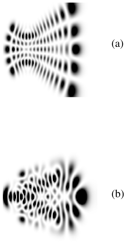
FIG. 1.: Typical eigenfunctions for the double-well potential in the (a) near-integrable case without Gaussian perturbations, $E=-11.055$, and (b) chaotic case with Gaussian perturbations, $E=-12.063$. Only one side of the well is shown in each case, with the $x$-axis running horizontally from $-6$ to 0 and the $y$-axis vertically from $-2$ to 2. The barrier is located on the right side at $x=0$.

FIG. 2.: Contour plot of the potential for a typical member of the ensemble. The perturbation at $x=\pm 2,y=\pm 1$ leads to a symmetrical distortion of the contours, which would be more rounded in the absence of a perturbation. The contours range from $V=-300$ near the bottom of the potential to $V=+200$ above the top of the barrier.

FIG. 3.: Level splitting versus energy $E$ for the 15195 eigenstates between $E=0$ and $E=-50$ in the ensemble of 625 double-well potentials described in the text.

FIG. 4.: Rescaled level splitting versus energy $E$ as in Fig. 3.

FIG. 5.: Rescaled level splitting versus action$/2\pi$ with eigenstates as in Fig. 3.

FIG. 6.: Rescaled level splitting versus the overlap of the eigenstate with a Gaussian on the horizontal periodic orbit, with eigenstates as in Fig. 3.

FIG. 7.: Overlap versus energy $E$, with eigenstates as in Fig. 3.

FIG. 8.: Mean rescaled splitting $s/\langle s\rangle$ versus action/$2\pi$, data points; short-time envelope from scar theory using Eq. (6), solid line; short-time envelope from scar theory using Eq. (5), dashed line.

FIG. 9.: Distribution of rescaled splittings for numerical data with $\sigma=0.5$, solid histogram; numerical data with $\sigma=0.63$, dashed histogram; Porter–Thomas distribution (without correction for finite $\hbar$, see Fig. 11), dashed line.

FIG. 10.: Plot of $\Delta E/e^{-S}$ versus mean level spacing $\Delta$.

FIG. 11.: Distribution of rescaled splittings for the numerical data with $\sigma=0.5$, histogram; Porter–Thomas distribution with finite-$\hbar$ correction for $N=6$, dashed line.

REFERENCES

- [1] Electronic address: bies@fas.harvard.edu.
- [2] R. Hernandez, W. H. Miller, C. Bradley Moore and W. F. Polik, J. Chem. Phys. 99, 950 (1993); W. H. Miller, R. Hernandez, C. B. Moore and W. F. Polik, J. Chem. Phys. 93, 5657 (1990); P. J. Robinson and K. A. Holbrook, Unimolecular Reactions (Wiley-Interscience, New York, 1972); J. I. Steinfeld, J. S. Francisco and W. L. Hase, Chemical Kinetics and Dynamics (Prentice Hall, Englewood Cliffs, N.J., 1989).
- [3] J. E. Lynn, The Theory of Neutron Resonance Reactions (Oxford, 1968).
- [4] C. E. Porter and R. G. Thomas, Phys. Rev. 104, 483 (1956).
- [5] L. P. Kouwenhoven, C. M. Marcus, P. L. Mceuen, S. Tarucha, R. M. Westervelt and N. S. Wingreen, ‘Electron transport in quantum dots,’ in Mesoscopic Electron Transport, ed. L. L. Sohn, L. P. Kouwenhoven and G. Schön, (Kluwer, 1997), pp. 105–214; C. M. Marcus, R. M. Westervelt, P. F. Hopkins and A. C. Gossard, Chaos 3, 643 (1993).
- [6] T. M. Fromhold, L. Eaves, F. W. Sheard, M. L. Leadbeater, T. J. Foster and P. C. Main, Phys. Rev. Lett. 72, 2608 (1994); P. B. Wilkinson, T. M. Fromhold, L. Eaves, F. W. Sheard, N. Miura and T. Takamasu, Nature 380, 608 (1996); T. M. Fromhold, P. B. Wilkinson, F. W. Sheard, L. Eaves, J. Miao and G. Edwards, Phys. Rev. Lett. 75, 1142 (1995).
- [7] D. Bohm, Quantum Theory (Prentice-Hall, New York, 1951), pp. 264–295.
- [8] S. C. Creagh and N. D. Whelan, Ann. Phys. 272, 196 (1999).
- [9] S. C. Creagh and N. D. Whelan, Phys. Rev. Lett. 84, 4084 (2000).
- [10] D. O. Harris, G. G. Engerholm and W. D. Gwinn, J. Chem. Phys. 43, 1515 (1965); for more recent work see J. V. Lill, G. A. Parker and J. C. Light, Chem. Phys. Lett. 89, 483 (1982); J. C. Light, I. P. Hamilton and J. V. Lill, J. Chem. Phys. 82, 1400 (1985).
- [11] L. Kaplan and E. J. Heller, Ann. Phys. 264, 171 (1998); see also the review: L. Kaplan, Nonlinearity 12, R1 (1999) and references therein.
- [12] O. Agam and S. Fishman, Phys. Rev. Lett. 73, 806 (1994); O. Agam and S. Fishman, J. Phys. A 26, 2113 (1993).
- [13] L. Kaplan, Phys. Rev. Lett. 80, 2582 (1998).
- [14] A. I. Schnirelman, Usp. Mat. Nauk. 29, 181 (1974); Y. Colin de Verdiere, Commun. Math. Phys. 102, 497 (1985); S. Zelditch, Duke Math. J. 55, 919 (1987); S. Zelditch and M. Zworski, Commun. Math. Phys. 175, 673 (1996).
- [15] L. Kaplan, Phys. Rev. E 59, 5325 (1999).
- [16] T. A. Brody, J. Flores, J. B. French, P. A. Mello, A. Pandey and S. S. M. Wong, Rev. Mod. Phys. 53, 385 (1981).